4.2 Wrangle metadata#
Introduction#
In the last notebook, we demonstrated reading a larger-than-memory dataset using GDAL virtual datasets. Building the GDAL virtual dataset combines the stack of images by assigning each image to a 'band' dimension. However, reading the data in this way caused important metadata to be lost. This notebook details steps of parsing metadata stored in filenames and separate files and formatting it so that it can be combined with the Xr.Dataset holding Sentinel-1 backscatter imagery, the physical observable we’re interested in.
A good first step here is to check out the README file that is located within each scene directory. This has important metadata that we need as well as instructions for how to interpret the file names. Check that out now if you haven’t yet.
We need to bring the information from the README files and the file names and organize it so that it is most useful to us as we try to interpret the Sentinel-1 backscatter imagery.
A. Read and inspect initial metadata
Add appropriate names to variables
What metadata currently exists?
B. Add metadata from file name
Parse file name
Extract and format acquisition dates
Combine data cubes
Extract attributes as list of dictionaries
Create tuple of metadata for each type of information
Assign metadata tuple to Xarray dataset as a coordinate variable
D. Add metadata from README file
Extract granule ID
Build coordinate
xr.DataArray
Concepts
Understand the connection between metadata and physical observable data.
Format information within a data cube so that metadata maximizes usability of data cube.
Understand processing attributes of Sentinel-1 imagery and file naming conventions.
Techniques
Parse strings in file names and markdown files using schema with regex expressions to ensure expected behavior.
Use Xarray coordinates and attributes to store different types of metadata.
Combine multiple raster data cubes with
xr.combine_by_coords().
Show code cell source
%load_ext rich
%xmode minimal

import cf_xarray
import markdown
import pandas as pd
import pathlib
import re
import xarray as xr

import s1_tools
Exception reporting mode: Minimal
cwd = pathlib.Path.cwd()
tutorial2_dir = pathlib.Path(cwd).parent
A. Read data and inspect initial metadata#
Attention
If you are following along on your own computer, be sure to specify two things:
Set ``path_to_rtcs` to the location of the downloaded files on your own computer.
Set
timeseries_typeto'full'or'subset'depending on if you are using the full time series (103 files) or the subset time series (5 files).
Read the VRT files using xr.open_dataset():
timeseries_type = "full"
path_to_rtcs = f"data/raster_data/{timeseries_type}_timeseries/asf_rtcs"
ds_vv = xr.open_dataset(
    f"../data/raster_data/{timeseries_type}_timeseries/vrt_files/s1_stack_vv.vrt",
    chunks="auto",
)
ds_vh = xr.open_dataset(
    f"../data/raster_data/{timeseries_type}_timeseries/vrt_files/s1_stack_vh.vrt",
    chunks="auto",
)
ds_ls = xr.open_dataset(
    f"../data/raster_data/{timeseries_type}_timeseries/vrt_files/s1_stack_ls_map.vrt",
    chunks="auto",
)
1) Rename band_data variables to appropriate names#
ds_vv = ds_vv.rename({"band_data": "vv"})
ds_vh = ds_vh.rename({"band_data": "vh"})
ds_ls = ds_ls.rename({"band_data": "ls"})
2) What metadata currently exists?#
Use cf_xarray to parse the metadata contained in the dataset.
ds_vv.cf
╭─ Coordinates ────────────────────────────────────────────────────────────────────────────────────╮
│              CF Axes:   X, Y, Z, T: n/a                                                          │
│                                                                                                  │
│       CF Coordinates:   longitude, latitude, vertical, time: n/a                                 │
│                                                                                                  │
│        Cell Measures:   area, volume: n/a                                                        │
│                                                                                                  │
│       Standard Names:   n/a                                                                      │
│                                                                                                  │
│               Bounds:   n/a                                                                      │
│                                                                                                  │
│        Grid Mappings:   transverse_mercator: ['spatial_ref']                                     │
╰──────────────────────────────────────────────────────────────────────────────────────────────────╯
╭─ Data Variables ─────────────────────────────────────────────────────────────────────────────────╮
│        Cell Measures:   area, volume: n/a                                                        │
│                                                                                                  │
│       Standard Names:   n/a                                                                      │
│                                                                                                  │
│               Bounds:   n/a                                                                      │
│                                                                                                  │
│        Grid Mappings:   n/a                                                                      │
╰──────────────────────────────────────────────────────────────────────────────────────────────────╯
As you can see, we’re lacking a lot of information, but we do have spatial reference information that allows us to understand how the data cube’s pixels correspond to locations on Earth’s surface (we also know this from the README file and the shp file in each scene’s directory).
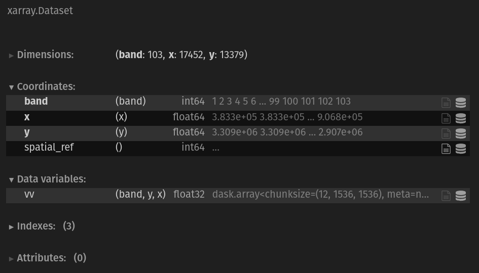
ds_vv
<xarray.Dataset> Size: 96GB
Dimensions:      (band: 103, x: 17452, y: 13379)
Coordinates:
  * band         (band) int64 824B 1 2 3 4 5 6 7 8 ... 97 98 99 100 101 102 103
  * x            (x) float64 140kB 3.833e+05 3.833e+05 ... 9.068e+05 9.068e+05
  * y            (y) float64 107kB 3.309e+06 3.309e+06 ... 2.907e+06 2.907e+06
    spatial_ref  int64 8B ...
Data variables:
vv (band, y, x) float32 96GB dask.array<chunksize=(12, 1536, 1536), meta=np.ndarray>The x and y dimensions have associated coordinate variables and there is a 'spatial_ref' variable that gives coordinate reference system information about those coordinates. In the attributes of 'spatial_ref', we see that our object is projected in local UTM (Universal Transverse Mercator) zone 45N. This tells us that the units of the coordinate arrays are meters. Read more about UTM zones here.
ds_vv["spatial_ref"].attrs
{
'crs_wkt': 'PROJCS["WGS 84 / UTM zone 45N",GEOGCS["WGS 84",DATUM["WGS_1984",SPHEROID["WGS 84",6378137,298.257223563,AUTHORITY["EPSG","7030"]],AUTHORITY["EPSG","6326"]],PRIMEM["Greenwich",0,AUTHORITY["EPSG","8901"]],UNIT["degree",0.0174532925199433,AUTHORITY["EPSG","9122"]],AUTHORITY["EPSG","4326"]],PROJECTION["Transverse_Mercator"],PARAMETER["latitude_of_origin",0],PARAMETER["central_meridian",87],PARAMETER["scale_factor",0.9996],PARAMETER["false_easting",500000],PARAMETER["false_northing",0],UNIT["metre",1,AUTHORITY["EPSG","9001"]],AXIS["Easting",EAST],AXIS["Northing",NORTH],AUTHORITY["EPSG","32645"]]',
'semi_major_axis': 6378137.0,
'semi_minor_axis': 6356752.314245179,
'inverse_flattening': 298.257223563,
'reference_ellipsoid_name': 'WGS 84',
'longitude_of_prime_meridian': 0.0,
'prime_meridian_name': 'Greenwich',
'geographic_crs_name': 'WGS 84',
'horizontal_datum_name': 'World Geodetic System 1984',
'projected_crs_name': 'WGS 84 / UTM zone 45N',
'grid_mapping_name': 'transverse_mercator',
'latitude_of_projection_origin': 0.0,
'longitude_of_central_meridian': 87.0,
'false_easting': 500000.0,
'false_northing': 0.0,
'scale_factor_at_central_meridian': 0.9996,
'spatial_ref': 'PROJCS["WGS 84 / UTM zone 45N",GEOGCS["WGS 84",DATUM["WGS_1984",SPHEROID["WGS 84",6378137,298.257223563,AUTHORITY["EPSG","7030"]],AUTHORITY["EPSG","6326"]],PRIMEM["Greenwich",0,AUTHORITY["EPSG","8901"]],UNIT["degree",0.0174532925199433,AUTHORITY["EPSG","9122"]],AUTHORITY["EPSG","4326"]],PROJECTION["Transverse_Mercator"],PARAMETER["latitude_of_origin",0],PARAMETER["central_meridian",87],PARAMETER["scale_factor",0.9996],PARAMETER["false_easting",500000],PARAMETER["false_northing",0],UNIT["metre",1,AUTHORITY["EPSG","9001"]],AXIS["Easting",EAST],AXIS["Northing",NORTH],AUTHORITY["EPSG","32645"]]',
'GeoTransform': '383250.0 30.0 0.0 3308730.0 0.0 -30.0'
}
Great, we know where our data is located in space. But, with the data in its current form, we don’t know much else about how or when it was collected. The rest of this notebook will demonstrate finding that information from both the file names of the individual files and the other files located in the scene directories.
B. Add metadata from file name#
Perhaps most importantly, we need to know when these observations were collected in time.
As we know from the README, information about acquisitions dates and more is stored in the directory name for each scene as well as the individual file names.
ds_vh.band
<xarray.DataArray 'band' (band: 103)> Size: 824B
array([  1,   2,   3,   4,   5,   6,   7,   8,   9,  10,  11,  12,  13,  14,
        15,  16,  17,  18,  19,  20,  21,  22,  23,  24,  25,  26,  27,  28,
        29,  30,  31,  32,  33,  34,  35,  36,  37,  38,  39,  40,  41,  42,
        43,  44,  45,  46,  47,  48,  49,  50,  51,  52,  53,  54,  55,  56,
        57,  58,  59,  60,  61,  62,  63,  64,  65,  66,  67,  68,  69,  70,
        71,  72,  73,  74,  75,  76,  77,  78,  79,  80,  81,  82,  83,  84,
        85,  86,  87,  88,  89,  90,  91,  92,  93,  94,  95,  96,  97,  98,
        99, 100, 101, 102, 103])
Coordinates:
* band (band) int64 824B 1 2 3 4 5 6 7 8 ... 97 98 99 100 101 102 103
spatial_ref int64 8B ...1) Parse file name#
The function below extracts metadata from the filename of each GeoTIFF file in the time series. It uses regex expressions to parse the different types of information stored within the file name based on the instructions from the README. Once parsed, the information is stored as a dictionary where each key is the type of information (ie. Acquisition start date and time, polarization, imaging mode, etc.) and each value is the corresponding information from the file name.
def parse_fname_metadata(input_fname: str) -> dict:
    """Function to extract information from filename and separate into expected variables based on a defined schema."""
    # Define schema
    schema = {
        "sensor": (3, r"S1[A-B]"),  # schema for sensor
        "beam_mode": (2, r"[A-Z]{2}"),  # schema for beam mode
        "acq_date": (15, r"[0-9]{8}T[0-9]{6}"),  # schema for acquisition date
        "pol_orbit": (3, r"[A-Z]{3}"),  # schema for polarization + orbit type
        "terrain_correction_pixel_spacing": (
            5,
            r"RTC[0-9]{2}",
        ),  # schema for terrain correction pixel spacing
        "processing_software": (
            1,
            r"[A-Z]{1}",
        ),  # schema for processing software (G = Gamma)
        "output_info": (6, r"[a-z]{6}"),  # schema for output info
        "product_id": (4, r"[A-Z0-9]{4}"),  # schema for product id
        "prod_type": ((2, 6), (r"[A-Z]{2}", r"ls_map")),  # schema for polarization type
    }

    # Remove prefixs
    input_fname = input_fname.split("/")[-1]
    # Remove file extension if present
    input_fname = input_fname.removesuffix(".tif")
    # Split filename string into parts
    parts = input_fname.split("_")

    # l-s map objects have an extra '_' in the filename. Remove/combine parts so that it matches schema
    if parts[-1] == "map":
        parts = parts[:-1]
        parts[-1] = parts[-1] + "_map"

    # Check that number of parts matches expected schema
    if len(parts) != len(schema):
        raise ValueError(f"Input filename does not match schema of expected format: {parts}")

    # Create dict to store parsed data
    parsed_data = {}

    # Iterate through parts and schema
    for part, (name, (length_options, pattern_options)) in zip(parts, schema.items()):
        # In the schema we defined, items have an int for length or a tuple (when there is more than one possible length)
        # Make the int lengths into tuples
        if isinstance(length_options, int):
            length_options = (length_options,)
        # Same as above for patterns
        if isinstance(pattern_options, str):
            pattern_options = (pattern_options,)

        # Check that each length of each part matches expected length from schema
        if len(part) not in length_options:
            raise ValueError(f"Part {part} does not have expected length {len(part)}")
        # Check that each part matches expected pattern from schema
        if not any(re.fullmatch(pattern, part) for pattern in pattern_options):
            raise ValueError(f"Part {part} does not match expected patterns {pattern_options}")

        # Special handling of a part (pol orbit) that has 3 types of metadata
        if name == "pol_orbit":
            parsed_data.update(
                {
                    "polarization_type": part[:1],  # Single (S) or Dual (D) pol
                    "primary_polarization": part[1:2],  # Primary polarization (H or V)
                    "orbit_type": part[-1],  # Precise (p), Restituted (r) or Original predicted (o)
                }
            )
        # Format string acquisition date as a datetime time stamp
        elif name == "acq_date":
            parsed_data[name] = pd.to_datetime(part, format="%Y%m%dT%H%M%S")
        # Expand multiple variables stored in output_info string part
        elif name == "output_info":
            output_info_keys = [
                "output_type",
                "output_unit",
                "unmasked_or_watermasked",
                "notfiltered_or_filtered",
                "area_or_clipped",
                "deadreckoning_or_demmatch",
            ]

            output_info_values = [part[0], part[1], part[2], part[3], part[4], part[-1]]

            parsed_data.update(dict(zip(output_info_keys, output_info_values)))

        else:
            parsed_data[name] = part

    # Because we have already addressed product type in the variable names
    prod_type = parsed_data.pop("prod_type")
    return parsed_data
Because we’ve already addressed product type (‘VV’ (dual-pol), ‘VH’(cross-pol), or ‘LS’ (layover-shadow)) in the variable names, we do not need to add it from the file name.
Note
We want to call parse_fname_metadata() on every GeoTIFF file in the time series. This means that we need the lists of file paths for each variable stored as GeoTIFF files that were created in the last notebook.
Before calling parse_fname_metadata(), we recreate the lists by calling the same functions used in the last notebook from s1_tools.
s1_asf_data = pathlib.Path(cwd.parent, path_to_rtcs)

variables_ls = ["vv", "vh", "ls_map", "readme"]
# Make dict
filepaths_dict = s1_tools.create_filenames_dict(s1_asf_data, variables_ls)
# Separate into lists
filepaths_vv, filepaths_vh, filepaths_ls, filepaths_rm = filepaths_dict.values()
2) Extract and format acquisition dates#
From each list of dictionaries created above, look at only the acq_date key, value pair in order to create lists of acquisition dates for each GeoTIFF file in the stack.
acq_dates_vh = [
    parse_fname_metadata(filepaths_vh[file])["acq_date"].strftime("%m/%d/%YT%H%M%S")
    for file in range(len(filepaths_vh))
]
acq_dates_vv = [
    parse_fname_metadata(filepaths_vv[file])["acq_date"].strftime("%m/%d/%YT%H%M%S")
    for file in range(len(filepaths_vv))
]
acq_dates_ls = [
    parse_fname_metadata(filepaths_ls[file])["acq_date"].strftime("%m/%d/%YT%H%M%S")
    for file in range(len(filepaths_ls))
]

# Make sure they are  equal
assert acq_dates_vh == acq_dates_vv == acq_dates_ls, "Acquisition dates lists for VH, VV and L-S Map do not match"
Let’s pause and return to the data we read at the very beginning and look at how it relates to the acquisition date metadata we just parsed.
In each data cube object (ds_vv, ds_vh and ds_ls), there is a 'band' dimension that has a length of 103. We know that this corresponds to time because of how we created the VRT files, but we don’t know anything else about the timing of the observations stored in the data cubes.
ds_vv
<xarray.Dataset> Size: 96GB
Dimensions:      (band: 103, x: 17452, y: 13379)
Coordinates:
  * band         (band) int64 824B 1 2 3 4 5 6 7 8 ... 97 98 99 100 101 102 103
  * x            (x) float64 140kB 3.833e+05 3.833e+05 ... 9.068e+05 9.068e+05
  * y            (y) float64 107kB 3.309e+06 3.309e+06 ... 2.907e+06 2.907e+06
    spatial_ref  int64 8B ...
Data variables:
vv (band, y, x) float32 96GB dask.array<chunksize=(12, 1536, 1536), meta=np.ndarray>We also just created three lists: acq_dates_vv, acq_dates_vh, and acq_dates_ls. Each element of these lists contains a datetime-like object:
print(acq_dates_vv[0])
02/14/2022T121353
We can assign these lists of dates to the data cubes using the xr.assign_coords() method together with pd.to_datetime(). pd.to_datetime() takes a string (the list elements) and turns it into a ‘time-aware’ object. `xr.assign_coords() assigns an array to a given coordinate.
ds_vv = ds_vv.assign_coords({"band": pd.to_datetime(acq_dates_vv, format="%m/%d/%YT%H%M%S")}).rename(
    {"band": "acq_date"}
)
ds_vh = ds_vh.assign_coords({"band": pd.to_datetime(acq_dates_vh, format="%m/%d/%YT%H%M%S")}).rename(
    {"band": "acq_date"}
)
ds_ls = ds_ls.assign_coords({"band": pd.to_datetime(acq_dates_ls, format="%m/%d/%YT%H%M%S")}).rename(
    {"band": "acq_date"}
)
In this case, we’re assigning the time-aware array produced by passing acq_dates_vv to pd.to_datetime() to the 'band' coordinate of the raster data cube.
3) Combine data cubes#
Up until this point, we’ve been working with three raster data cube objects, one for each variable (vv, vh and ls). We can combine them into one data cube with multiple variables using xr.combine_by_coords()
ds = xr.combine_by_coords([ds_vv, ds_vh, ds_ls])
As discussed in the first notebook, the scenes are not read in temporal order when the VRT objects were created, which is why the current data cube is not in temporal order. This is okay, because while the scenes were not in temporal order, they were read in the same order across all variables, which is why we could create and assign the time dimensions (acq_date) as we did and merge the individual objects into one data cube.
Now, let’s use xr.sortby() to arrange the data cube’s time dimension in chronological order.
ds = ds.sortby("acq_date")
ds
<xarray.Dataset> Size: 289GB
Dimensions:      (x: 17452, y: 13379, acq_date: 103)
Coordinates:
  * x            (x) float64 140kB 3.833e+05 3.833e+05 ... 9.068e+05 9.068e+05
  * y            (y) float64 107kB 3.309e+06 3.309e+06 ... 2.907e+06 2.907e+06
    spatial_ref  int64 8B 0
  * acq_date     (acq_date) datetime64[ns] 824B 2021-05-02T12:14:14 ... 2022-...
Data variables:
    ls           (acq_date, y, x) float32 96GB dask.array<chunksize=(11, 1536, 1536), meta=np.ndarray>
    vh           (acq_date, y, x) float32 96GB dask.array<chunksize=(11, 1536, 1536), meta=np.ndarray>
vv (acq_date, y, x) float32 96GB dask.array<chunksize=(11, 1536, 1536), meta=np.ndarray>C. Time-varying metadata#
So far we’ve only used the acquisition dates extracted from the file names, but the function we wrote parse_fname_metadata() holds additional information about how the scenes were imaged and processed.
Similarly to how we attached the acquisition date information to the raster data cubes, we’d also like to organize the imaging and processing metadata so that it is stored in relation to the raster imagery in a way that helps us interpret the raster imagery.
Remember that we have a dictionary of metadata attributes for each step of the time series and each variable (product type).
parse_fname_metadata(filepaths_vv[0])
{
    'sensor': 'S1A',
    'beam_mode': 'IW',
    'acq_date': Timestamp('2022-02-14 12:13:53'),
    'polarization_type': 'D',
    'primary_polarization': 'V',
    'orbit_type': 'P',
    'terrain_correction_pixel_spacing': 'RTC30',
    'processing_software': 'G',
    'output_type': 'g',
    'output_unit': 'p',
    'unmasked_or_watermasked': 'u',
    'notfiltered_or_filtered': 'n',
    'area_or_clipped': 'e',
    'deadreckoning_or_demmatch': 'd',
    'product_id': '51E7'
}
Rather than store this information as attrs of the data cube as a whole (ds.attrs) or individual data variables(ds['vv'].attrs), this information should be stored as coordinate variables of the data cube. This way, there is a coordinate name (the key of each dict item) and an array that holds the value at each time step.
The next several steps demonstrate how to execute this.
1) Extract metadata from file name for each GeoTIFF file#
Because product type is handled in the variable names, it isn’t necessary to extract from the filename. We’ll verify that the parsed metadata dictionaries are identical across variables and then move forward with only one list of metadata dictionaries. To do this, apply parse_fname_metadata() to each element of each variable list, making a list of dictionaries.
meta_attrs_list_vv = [parse_fname_metadata(filepaths_vv[file]) for file in range(len(filepaths_vv))]

meta_attrs_list_vh = [parse_fname_metadata(filepaths_vh[file]) for file in range(len(filepaths_vh))]

meta_attrs_list_ls = [parse_fname_metadata(filepaths_ls[file]) for file in range(len(filepaths_ls))]
Ensure that they are all identical:
assert (
    meta_attrs_list_ls == meta_attrs_list_vh == meta_attrs_list_vv
), "Lists of metadata dicts should be identical for all variables"
Now we can use only one list moving forward.
2) Re-organize lists of metadata dictionaries#
To assign coordinate variables to an Xarray dataset, the metadata needs to be re-organized a bit more. Currently, we have lists of 103 dictionaries with identical keys; each key will become a coordinate variable. We need to transpose the initial list of dictionaries; instead of a list of 103 dictionaries with 14 keys, we want a dictionary with 14 keys where each value is a 103-element long list.
def transpose_metadata_dict_list(input_ls: list) -> dict:
    df_ls = []
    # Iterate through list
    for element in range(len(input_ls)):
        # Create a dataframe of each dict in the list
        item_df = pd.DataFrame(input_ls[element], index=[0])
        df_ls.append(item_df)
    # Combine dfs row-wise into one df
    attr_df = pd.concat(df_ls)
    # Separate out each column in df to its own dict
    attrs_dict = {col: attr_df[col].tolist() for col in attr_df.columns}
    # Acq_dates are handled separately since we will use it as an index
    acq_date_ls = attrs_dict.pop("acq_date")
    return (attrs_dict, acq_date_ls)
attr_dict, acq_dt_list = transpose_metadata_dict_list(meta_attrs_list_vv)
3) Create xr.Dataset with metadata as coordinate variables#
We’ve re-organized the metadata into a format that Xarray expects for a xr.DataArray object. Because we will create a coordinate xr.DataArray for each metadata key, we write a function to repeat the operation:
def create_da(value_name: str, values_ls: list, dim_name: str, dim_values: list, desc: str = None) -> xr.DataArray:
    """Given a list of metadata values, create a 1-d xr.DataArray with values
    as data that exists along a specified dimension (here, hardcoded to be
    acq_date). Optionally, add description of metadata as attr.
    Returns a xr.DataArray"""
    da = xr.DataArray(
        data=values_ls,
        dims=[dim_name],
        coords={dim_name: dim_values},
        name=value_name,
    )
    if desc != None:
        da.attrs = {"description": desc}
    return da
Apply it to all of the metadata keys and then combine the xr.DataArray objects into a xr.Dataset.
def create_metadata_ds(dict_of_attrs: dict, list_of_acq_dates: list) -> xr.Dataset:
    da_ls = []
    for key in dict_of_attrs.keys():
        da = create_da(key, dict_of_attrs[key], "acq_date", list_of_acq_dates)
        da_ls.append(da)

    coord_ds = xr.combine_by_coords(da_ls)
    coord_ds = coord_ds.sortby("acq_date")
    return coord_ds
coord_ds = create_metadata_ds(attr_dict, acq_dt_list)
coord_ds
<xarray.Dataset> Size: 11kB
Dimensions:                           (acq_date: 103)
Coordinates:
  * acq_date                          (acq_date) datetime64[ns] 824B 2021-05-...
Data variables: (12/14)
    area_or_clipped                   (acq_date) <U1 412B 'e' 'e' ... 'e' 'e'
    beam_mode                         (acq_date) <U2 824B 'IW' 'IW' ... 'IW'
    deadreckoning_or_demmatch         (acq_date) <U1 412B 'd' 'd' ... 'd' 'd'
    notfiltered_or_filtered           (acq_date) <U1 412B 'n' 'n' ... 'n' 'n'
    orbit_type                        (acq_date) <U1 412B 'P' 'P' ... 'P' 'P'
    output_type                       (acq_date) <U1 412B 'g' 'g' ... 'g' 'g'
    ...                                ...
    primary_polarization              (acq_date) <U1 412B 'V' 'V' ... 'V' 'V'
    processing_software               (acq_date) <U1 412B 'G' 'G' ... 'G' 'G'
    product_id                        (acq_date) <U4 2kB '1424' ... 'E5B6'
    sensor                            (acq_date) <U3 1kB 'S1A' 'S1A' ... 'S1A'
    terrain_correction_pixel_spacing  (acq_date) <U5 2kB 'RTC30' ... 'RTC30'
unmasked_or_watermasked (acq_date) <U1 412B 'u' 'u' ... 'u' 'u'Great, we successfully extracted the data from the file names, organized it as dictionaries and created a xr.Dataset that holds all of the information organized along the appropriate dimension. The last step is to assign the data variables in coord_ds to be coordinate variables.
coord_ds = coord_ds.assign_coords({k: v for k, v in dict(coord_ds.data_vars).items()})
coord_ds
<xarray.Dataset> Size: 11kB
Dimensions:                           (acq_date: 103)
Coordinates: (12/15)
  * acq_date                          (acq_date) datetime64[ns] 824B 2021-05-...
    area_or_clipped                   (acq_date) <U1 412B 'e' 'e' ... 'e' 'e'
    beam_mode                         (acq_date) <U2 824B 'IW' 'IW' ... 'IW'
    deadreckoning_or_demmatch         (acq_date) <U1 412B 'd' 'd' ... 'd' 'd'
    notfiltered_or_filtered           (acq_date) <U1 412B 'n' 'n' ... 'n' 'n'
    orbit_type                        (acq_date) <U1 412B 'P' 'P' ... 'P' 'P'
    ...                                ...
    primary_polarization              (acq_date) <U1 412B 'V' 'V' ... 'V' 'V'
    processing_software               (acq_date) <U1 412B 'G' 'G' ... 'G' 'G'
    product_id                        (acq_date) <U4 2kB '1424' ... 'E5B6'
    sensor                            (acq_date) <U3 1kB 'S1A' 'S1A' ... 'S1A'
    terrain_correction_pixel_spacing  (acq_date) <U5 2kB 'RTC30' ... 'RTC30'
    unmasked_or_watermasked           (acq_date) <U1 412B 'u' 'u' ... 'u' 'u'
Data variables:
*empty*Next, combine them with the original data cube of backscatter imagery.
4) Combine data cube xr.Dataset with coordinate xr.Dataset#
ds_w_metadata = xr.merge([ds, coord_ds])
ds_w_metadata
<xarray.Dataset> Size: 289GB
Dimensions:                           (x: 17452, y: 13379, acq_date: 103)
Coordinates: (12/18)
  * x                                 (x) float64 140kB 3.833e+05 ... 9.068e+05
  * y                                 (y) float64 107kB 3.309e+06 ... 2.907e+06
    spatial_ref                       int64 8B 0
  * acq_date                          (acq_date) datetime64[ns] 824B 2021-05-...
    area_or_clipped                   (acq_date) <U1 412B 'e' 'e' ... 'e' 'e'
    beam_mode                         (acq_date) <U2 824B 'IW' 'IW' ... 'IW'
    ...                                ...
    primary_polarization              (acq_date) <U1 412B 'V' 'V' ... 'V' 'V'
    processing_software               (acq_date) <U1 412B 'G' 'G' ... 'G' 'G'
    product_id                        (acq_date) <U4 2kB '1424' ... 'E5B6'
    sensor                            (acq_date) <U3 1kB 'S1A' 'S1A' ... 'S1A'
    terrain_correction_pixel_spacing  (acq_date) <U5 2kB 'RTC30' ... 'RTC30'
    unmasked_or_watermasked           (acq_date) <U1 412B 'u' 'u' ... 'u' 'u'
Data variables:
    ls                                (acq_date, y, x) float32 96GB dask.array<chunksize=(11, 1536, 1536), meta=np.ndarray>
    vh                                (acq_date, y, x) float32 96GB dask.array<chunksize=(11, 1536, 1536), meta=np.ndarray>
vv (acq_date, y, x) float32 96GB dask.array<chunksize=(11, 1536, 1536), meta=np.ndarray>Great, from a stack of files that make up a raster time series, we figured out how to take information stored in a every file name and assign it as non-dimensional coordinate variables of the data cube representing the raster time series.
While it’s good that we did this because there is nothing ensuring that the metadata in the file names is identical across time steps, many of these attributes are identical across the time series. This means that we can handle them more simply as attributes rather than coordinate variables, though we will still keep some metadata as coordinates.
First, verify which metadata attributes are identical throughout the time series:
# Make list of coords that are along time dimension
coords_along_time_dim = [coord for coord in ds_w_metadata._coord_names if "acq_date" in ds_w_metadata[coord].dims]
dynamic_attrs = []
static_attr_dict = {}
for i in coords_along_time_dim:
    if i != "acq_date":
        # find coordinate array variables that have more than
        # one unique element along time dimension
        if len(set(ds_w_metadata.coords[i].data.tolist())) > 1:
            dynamic_attrs.append(i)
        else:
            static_attr_dict[i] = ds_w_metadata.coords[i].data[0]
Drop the static coordinates from the data cube:
ds_w_metadata = ds_w_metadata.drop_vars(list(static_attr_dict.keys()))
And add them as attributes:
ds_w_metadata.attrs = static_attr_dict
ds_w_metadata
<xarray.Dataset> Size: 289GB
Dimensions:      (x: 17452, y: 13379, acq_date: 103)
Coordinates:
  * x            (x) float64 140kB 3.833e+05 3.833e+05 ... 9.068e+05 9.068e+05
  * y            (y) float64 107kB 3.309e+06 3.309e+06 ... 2.907e+06 2.907e+06
    spatial_ref  int64 8B 0
  * acq_date     (acq_date) datetime64[ns] 824B 2021-05-02T12:14:14 ... 2022-...
    product_id   (acq_date) <U4 2kB '1424' '54B1' '8A4F' ... '1380' 'E5B6'
Data variables:
    ls           (acq_date, y, x) float32 96GB dask.array<chunksize=(11, 1536, 1536), meta=np.ndarray>
    vh           (acq_date, y, x) float32 96GB dask.array<chunksize=(11, 1536, 1536), meta=np.ndarray>
    vv           (acq_date, y, x) float32 96GB dask.array<chunksize=(11, 1536, 1536), meta=np.ndarray>
Attributes: (12/13)
    area_or_clipped:                   e
    notfiltered_or_filtered:           n
    orbit_type:                        P
    sensor:                            S1A
    beam_mode:                         IW
    terrain_correction_pixel_spacing:  RTC30
    ...                                ...
    polarization_type:                 D
    output_unit:                       p
    processing_software:               G
    output_type:                       g
    deadreckoning_or_demmatch:         d
primary_polarization: VD. Add metadata from README file#
Until now, all of the attribute information that we’ve added to the data cube came from file names of the individual scenes that make up the data cube. One piece of information not included in the file name is the original granule ID of the scene published by ESA. This is information about the source image, produced by ESA, and used by ASF when processing a SLC image into a RTC image. This is located in the README file within each scene directory.
Having the granule ID can be helpful because it tells you if the satellite was in an ascending or a descending cycle when the image was captured. For surface conditions with diurnal fluctuations such as snowmelt, the timing of the image acquisition may be important.
Note
This notebook works through the steps to format and organize metadata while explaining the details behind these operations. It is meant to be an educational demonstration. There are packages available such as Sentinelsat that simplify metadata retrieval of Sentinel-1 imagery.
1) Extract granule ID#
We first need to extract the text containing a scene’s granule ID from that scene’s README file. This is similar to parsing the file and directory names but this time we’re extracting text from a markdown file. To do this, we use the python-markdown package. From looking at the file, we know where the source granule information is located; we need to isolate it from the rest of the text in the file. The source granule information always follows the same pattern, so we can use string methods to extract it.
def extract_granule_id(filepath):
    """takes a filepath to the readme associated with an S1 scene and returns the source granule id used to generate the RTC imagery"""

    # Use markdown package to read text from README
    md = markdown.Markdown(extensions=["meta"])
    # Extract text from file
    data = pathlib.Path(filepath).read_text()
    # this text precedes granule ID in readme
    pre_gran_str = "The source granule used to generate the products contained in this folder is:\n"
    split = data.split(pre_gran_str)
    # isolate the granule id
    gran_id = split[1][:67]

    return gran_id
Before moving on, take a look at a single source granule ID string:
Show code cell source
granule_ls = [extract_granule_id(filepaths_rm[element]) for element in range(len(filepaths_rm))]
granule_ls[0]
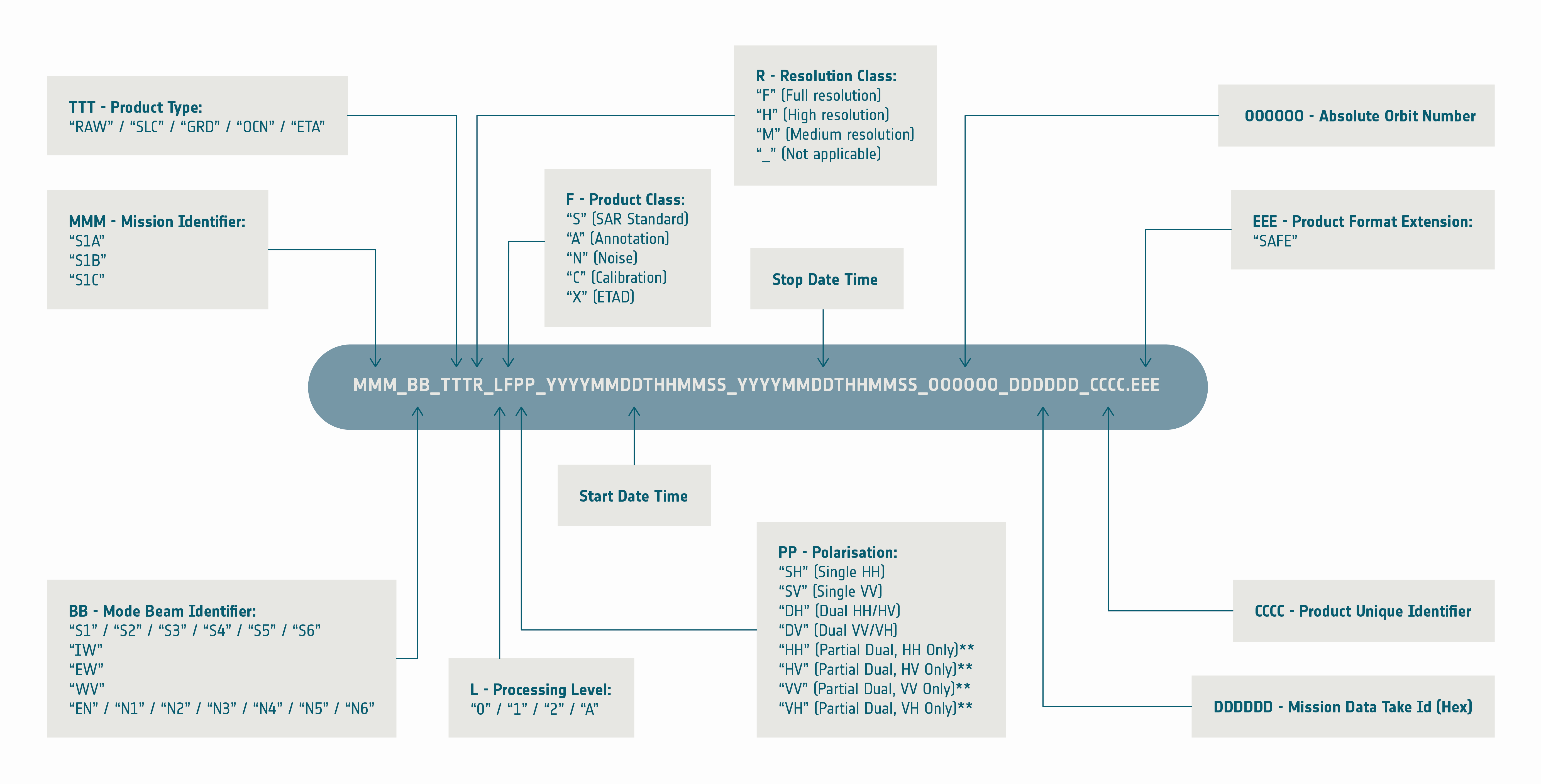
'S1A_IW_SLC__1SDV_20220214T121353_20220214T121420_041909_04FD6F_42AF'
Below is information from the ESA’s SentiWiki on Sentinel-1 Product Naming Conventions. In addition to the sensor and the beam mode, it tells us that the product type is a ‘Single Look Complex’ (SLC) image and is Level-1 processed data. The two date-time like sections indicate the start (14 February 2022, 12:13:53) and stop (14 February 2022, 12:14:20) date and time of the observation which are followed by the absolute orbit number (041909), a mission data take ID (04FD6F) and a unique product ID (42AF).
2) Build granule ID coordinate array#
This is another situation of time-varying metadata. Once we have the individual granule IDs, we must format them so that they can be attached to an Xarray object. We use a similar schema approach to parsing the file names:
def make_coord_data(readme_fpaths_ls):
    """takes a list of the filepaths to every read me, extracts the granule ID.
    From granule ID, extracts acquisition date and data take ID.
    Returns a tuple of lists of acquisition dates and data take IDs."""

    # Make a list of all granules in time series
    granule_ls = [extract_granule_id(readme_fpaths_ls[element]) for element in range(len(readme_fpaths_ls))]
    # Define a schema for acquisition date
    schema = {
        "mission_identifier": (3, r"S1[A-B]"),  # schema for sensor
        "mode_beam_identifier": (2, r"[A-Z]{2}"),  # schema for beam mode
        "esa_product_type": (3, r"[A-Z]{3}"),  # schema for ESA product type
        "proc_lvl_class_pol": (4, r"[A-Z0-9]{{4}}"),
        "acq_start": (15, r"[0-9]{8}T[0-9]{6}"),  # schema for acquisition dat
        "acq_stop": (15, r"[0-9]{8}T[0-9]{6}"),  # schema for acquisition dat
        "orbit_num": (6, r"[0-9]{6}"),  # schema for orbit number
        "data_take_id": (6, "A-Z0-9{6}"),  # schema for data take id
    }

    # Extract relevant metadata from granule ID
    all_granules_parsed_data = []
    for granule in granule_ls:
        # need to account for double under score
        parts = [s for s in granule.split("_") if len(s) > 0]
        # parts = granule.split("_")
        single_granule_parsed_data = {}
        for part, (name, (length, pattern)) in zip(parts, schema.items()):
            if name == "acq_start":
                single_granule_parsed_data["acq_start"] = pd.to_datetime(part, format="%Y%m%dT%H%M%S")
            elif name == "orbit_num":
                single_granule_parsed_data[name] = part
            elif name == "data_take_id":
                single_granule_parsed_data[name] = part
        all_granules_parsed_data.append(single_granule_parsed_data)

    acq_dates = [granule["acq_start"] for granule in all_granules_parsed_data]
    abs_orbit_no = [granule["orbit_num"] for granule in all_granules_parsed_data]
    data_take_ids = [granule["data_take_id"] for granule in all_granules_parsed_data]

    return (acq_dates, abs_orbit_no, data_take_ids)
acquisition_dates, abs_orbit_ls, data_take_ids_ls = make_coord_data(filepaths_rm)
Reuse the create_da() function that we used above:
data_take_id_da = create_da(
    value_name="data_take_id",
    values_ls=data_take_ids_ls,
    dim_name="acq_date",
    dim_values=acquisition_dates,
    desc="ESA Mission data take ID",
)
Make sure data_take_id_da is sorted in chronological order:
data_take_id_da = data_take_id_da.sortby("acq_date")
Add the xr.DataArray of ESA data take IDs to raster data cube of Sentinel-1 scenes as a coordinate variable:
ds_w_metadata.coords["data_take_ID"] = data_take_id_da
Repeat the above steps to add absolute orbit number as a coordinate variable to the data cube:
# Create DatArray
abs_orbit_da = create_da(
    value_name="abs_orbit_num",
    values_ls=abs_orbit_ls,
    dim_name="acq_date",
    dim_values=acquisition_dates,
    desc="Absolute orbit number",
)
# Sort by time
abs_orbit_da = abs_orbit_da.sortby("acq_date")
# Add as coord variable to data cube
ds_w_metadata.coords["abs_orbit_num"] = abs_orbit_da
ds_w_metadata
<xarray.Dataset> Size: 289GB
Dimensions:        (x: 17452, y: 13379, acq_date: 103)
Coordinates:
  * x              (x) float64 140kB 3.833e+05 3.833e+05 ... 9.068e+05 9.068e+05
  * y              (y) float64 107kB 3.309e+06 3.309e+06 ... 2.907e+06 2.907e+06
    spatial_ref    int64 8B 0
  * acq_date       (acq_date) datetime64[ns] 824B 2021-05-02T12:14:14 ... 202...
    product_id     (acq_date) <U4 2kB '1424' '54B1' '8A4F' ... '1380' 'E5B6'
    data_take_ID   (acq_date) <U6 2kB '047321' '047463' ... '052C00' '052C00'
    abs_orbit_num  (acq_date) <U6 2kB '037709' '037745' ... '043309' '043309'
Data variables:
    ls             (acq_date, y, x) float32 96GB dask.array<chunksize=(11, 1536, 1536), meta=np.ndarray>
    vh             (acq_date, y, x) float32 96GB dask.array<chunksize=(11, 1536, 1536), meta=np.ndarray>
    vv             (acq_date, y, x) float32 96GB dask.array<chunksize=(11, 1536, 1536), meta=np.ndarray>
Attributes: (12/13)
    area_or_clipped:                   e
    notfiltered_or_filtered:           n
    orbit_type:                        P
    sensor:                            S1A
    beam_mode:                         IW
    terrain_correction_pixel_spacing:  RTC30
    ...                                ...
    polarization_type:                 D
    output_unit:                       p
    processing_software:               G
    output_type:                       g
    deadreckoning_or_demmatch:         d
primary_polarization: VE. 3-d metadata#
The metadata we’ve looked at so far has been information related to how and when the image was processed. An element of the dataset we haven’t focused on yet is the layover shadow map provided by ASF. This is an important tool for interpreting backscatter imagery that we’ll discuss in more detail in the next notebook. What’s important to know at this step is that the layover-shadow map is provided for every scene in the time series and contains a number assignment for each pixel in the scene that indicates the presence or absence of layover, shadow, and slope angle conditions that impact backscatter values.
This means that the layover-shadow map is a raster image in itself that helps us interpret the raster images of backscatter values. Because it is metadata that gives context to the physical observable (backscatter) and it varies over spatial and temporal dimensions, it is most appropriately represented as a coordinate variable of the data cube:
ds_w_metadata = ds_w_metadata.set_coords("ls")
ds_w_metadata
<xarray.Dataset> Size: 289GB
Dimensions:        (x: 17452, y: 13379, acq_date: 103)
Coordinates:
  * x              (x) float64 140kB 3.833e+05 3.833e+05 ... 9.068e+05 9.068e+05
  * y              (y) float64 107kB 3.309e+06 3.309e+06 ... 2.907e+06 2.907e+06
    spatial_ref    int64 8B 0
    ls             (acq_date, y, x) float32 96GB dask.array<chunksize=(11, 1536, 1536), meta=np.ndarray>
  * acq_date       (acq_date) datetime64[ns] 824B 2021-05-02T12:14:14 ... 202...
    product_id     (acq_date) <U4 2kB '1424' '54B1' '8A4F' ... '1380' 'E5B6'
    data_take_ID   (acq_date) <U6 2kB '047321' '047463' ... '052C00' '052C00'
    abs_orbit_num  (acq_date) <U6 2kB '037709' '037745' ... '043309' '043309'
Data variables:
    vh             (acq_date, y, x) float32 96GB dask.array<chunksize=(11, 1536, 1536), meta=np.ndarray>
    vv             (acq_date, y, x) float32 96GB dask.array<chunksize=(11, 1536, 1536), meta=np.ndarray>
Attributes: (12/13)
    area_or_clipped:                   e
    notfiltered_or_filtered:           n
    orbit_type:                        P
    sensor:                            S1A
    beam_mode:                         IW
    terrain_correction_pixel_spacing:  RTC30
    ...                                ...
    polarization_type:                 D
    output_unit:                       p
    processing_software:               G
    output_type:                       g
    deadreckoning_or_demmatch:         d
primary_polarization: VConclusion#
This notebook walked through an in-depth example of what working with real-world datasets can look like and the steps that are required to prepare data for analysis. We went from individual datasets for each variables that lacked important information about physical observables:
To a single data cube containing all three variables with a temporal dimension of np.datetime64 objects and additional metadata formatted as both coordinate variables and attributes depending on if it is static in time or not. It will now be much easier to make use of the dataset’s metadata in our analysis whether that is querying by time or space, performing computations on multiple variables at a time or filtering by unique ID’s of the processed and source datasets.