2.2 Data cubes

2.2 Data cubes#

The term data cube is used frequently throughout this book. This page contains an introduction of what a data cube is and why it is useful as well as how it connects to concepts such as ‘analysis-ready data’ and ‘data tidying.’

Anatomy of a data cube#

The key object of analysis in this book is a raster data cube. Raster data cubes are n-dimensional objects that store continuous measurements or estimates of physical quantities that exist along given dimension(s). Many scientific workflows involve examining how a variable (such as temperature, windspeed, relative humidity, etc.) varies over time and/or space. Data cubes are a way of organizing geospatial data that let us ask these questions.

A very common data cube structure is a 3-dimensional object with (x,y,time) dimensions (Baumann et al. [4], Giuliani et al. [19], Mahecha et al. [36], Montero et al. [40]). While this is a relatively intuitive concept,in practice, the amount and types of information contained within a single dataset and the operations involved in managing them, can become complicated and unwieldy. As analysts, we access data (usually from providers such as Distributed Active Archive Center or DAACs), and then we are responsible for organizing the data in a way that let’s us ask questions of it. While some of these decisions are straightforward (eg. It makes sense to stack observations from different points in time along a time dimension), some can be more open-ended (Where and how should important metadata be stored so that it will propagate across appropriate operations and be accessible when it is needed?).

Two types of information#

Fundamentally, many of these complexities can be reduced to one distinction: is a particular piece of information a physical observable (the main focus, or target, of the dataset), or is it metadata that provides necessary information in order to properly interpret and handle the physical observable 1? Answering this question will help you understand how to situate a piece of information within the broader data object.

An example dataset as a Xarray cube#

Imagine we have a time series of NDVI imagery generated from a stack of Landsat scenes. Before a user accesses a satellite imagery dataset, it has likely already undergone many levels of processing, transformation and re-organization. For more background on these steps, see Montero et al. Montero et al. [40], Section 3: ‘The Earth System Data Cube Life cycle’.

In this example, we’re accessing the dataset at a common dissemination point, an ‘image collection’2. It looks something like this:

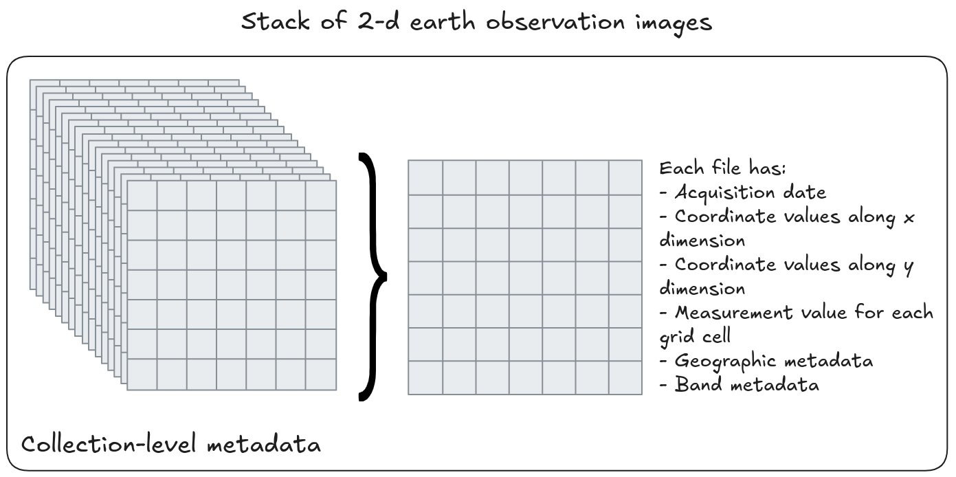
../_images/image_stack.png — Fig. 2 Illustration of earth observation time series as a stack of 2-d images and associated metadata.#

Without coordinate information and metadata, the image data are abstract arrays, meaning that we don’t know anything about the spatial or temporal location of the conditions they describe.

To use this data for scientific analysis, we need to construct it into the form of a cube. This requires a comprehensive understanding of the different pieces of information contained in the dataset and how they relate to one another in order to map the components of the dataset onto a cube structure.

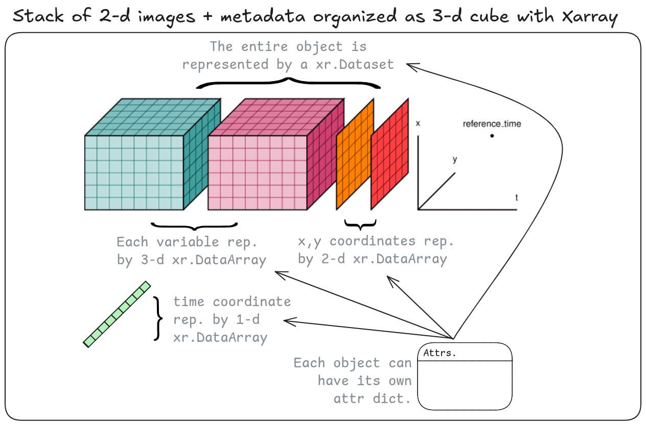
../_images/cube.png — Fig. 3 Illustration of earth observation time series organized as a 3-d Xarray data cube. Source: Adapted from Xarray Dev.#

In the context of the Xarray data model, univariate data cubes can be represented by an xr.DataArray or a xr.Dataset with one data_variable. Multivariate data cubes should be represented by xr.Dataset objects. The building blocks of xr.DataArrays and xr.Datasets are dimensions, coordinates, data variables, attributes. We recommend the Xarray terminology for a detailed overview of Xarray objects and common operations.

We’ve just discussed what a data cube is in the context of a standard earth observation dataset and how to use the Xarray data model to efficiently represent this kind of data. Another way of describing those steps is preparing the dataset so that it is fit for analysis.

‘Data Tidying’ and preparing data for analysis#

The topic of how to prepare data for analysis has received significant attention as an area of research in itself for at least two decades (Dasu and Johnson [11]). Dasu & Johnson motivate their discussion with the admonishment that a failure to adequately clean one’s data will almost certainly lead to flawed results, and many emphasize the considerable amount of time, effort and experience that this process can require (Dasu and Johnson [11], Wickham [54]).

In the tabular data domain, ‘tidy data’ has emerged as a robust framework for structuring data in order to simplify subsequent analysis. In this setting, a a tidy dataset is one where “each variable is a column, each observation is a row, and each type of observational unit is a table” (Wickham [54]). One way of describing such an object is that the dataset’s physical layout matches its semantic meaning (Wickham [54]). Wickham (2014) notes “tidy datasets are all alike but every messy dataset is messy in its own way” [54], underscoring the wide, and thus potentially complicated and confusing, range of steps needed to arrive at a ‘tidy’ dataset.

In the world of multi-dimensional gridded datasets, the ‘data cube’ structure achieves the closest symmetry between physical layout and semantic meaning (Gray et al. [21]), and has been identified as a core element of analysis-ready earth observation data (Baumann [3], Baumann et al. [4], Giuliani et al. [19]).

‘Analysis-ready data’#

The process described above is an example of preparing data for analysis. Thanks to development and collaboration across the earth observation community, analysis-ready for earth observation has a specific, technical definition:

CEOS Analysis Ready Data (CEOS-ARD) are satellite data that have been processed to a minimum set of requirements and organized into a form that allows immediate analysis with a minimum of additional user effort and interoperability both through time and with other datasets.
- Committee on Earth Observation Satellites (CEOS) Analysis-Ready Data [32]

Alongside the definition of the ARD specification has been the development and increasing availability of analysis-ready datasets and pipelines to produce them (Chatenoux et al. [7], Frantz [12], Killough [28], Stern et al. [48], Truckenbrodt et al. [52]), which represent exciting and transformative opportunities to increase the utilization and impact of earth observation datasets.

However, many legacy datasets still require significant effort in order to be considered ‘analysis-ready’. Furthermore, for analysts, ‘analysis-ready’ can be a subjective and evolving label. Semantically, from a user-perspective, analysis-ready data can be thought of as data whose structure is conducive to the analysis the user would like to perform.

Analysis-ready data cubes & this book#

This book’s tutorials use datasets that have been developed and released during this transition to open and cloud-based science and emphasis on analysis-ready data, and illustrate many of the concepts described so far in this section.

The ITS_LIVE tutorial features a dataset of multi-sensor observations that is already organized as a (x,y,time) cube on a common grid. In this case, much of the ‘tidying’ has been done for us, but as the notebooks show, a fair amount of manipulation and re-organization still is needed as we explore the dataset.

In the second tutorial, we work with two Sentinel-1 RTC datasets. Both have already undergone preprocessing using cloud-based compute resources to transform raw radar returns in slant range to a normalized backscatter coefficient. One dataset, Microsoft Planetary Computer Sentinel-1 RTC, is accessed as a (x,y,time) cube and one, processed using ASF’s HyP3 pipeline is accessed as a directory of files associated with individual scenes (single observations) and must be assembled into a (x,y,time) cube. In this example, we highlight the importance of a detailed understanding of the data in order to direct appropriate and robust analysis, and demonstrate the programmatic steps involved in ‘tidying’ a set of discrete observations into a (x,y,time) cube.