2.4 Data used in tutorials

We use a many different datasets throughout these tutorials. While each tutorial is focused on a different raster time series (ITS_LIVE ice velocity data and Sentinel-1 imagery), we also use vector data to represent points of interest.

Most of the examples in this book use data accessed programmatically from cloud-object storage. We make subset of the data available in this books Github repository to remove the need for computationally-intensive operations in the tutorials. In one example, working with Sentinel-1 data processed by Alaska Satellite Facility, we start with data downloaded locally. Users who would like to complete this processing step on their own may do so (and access the data here), but a smaller subset of this data is stored in the repository.

Here is a broad overview the data included in this tutorial, including how it is collected, it’s potential scientific applications, and how and where it is stored and accessed in these tutorials.

Inter-mission Time Series of Land Ice Velocity and Elevation (ITS_LIVE)

Dataset name	Produced by	Storage format	Storage location
ITS_LIVE	ITS_LIVE project, NASA JPL	Zarr	AWS S3

ITS_LIVE is a dataset of ice velocity observations derived from applying a feature tracking algorithm to pairs of satellite imagery. Ice velocity refers to the down-slope movement of glaciers and ice sheets [13]. Because glaciers and ice sheets are dynamic elements of our climate system, they lose or gain mass in response to changes in climate conditions such as warmer temperatures or increased snowfall, measuring variability in the speed of ice flow can help scientists better understand trends in glacier dynamics and interactions between glaciers and climate.

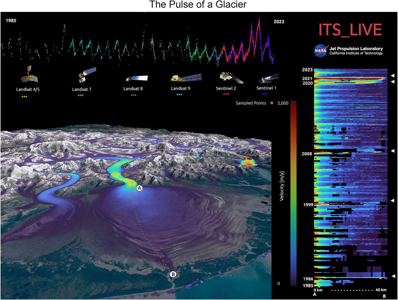
Fig. 4 Example of a ice velocity time series along centerline profile of Malaspina Glacier featuring velocity observations from a range of satellite sensors. Source: Reproduced with permission from Lopez et al. [33].

Part of what is so exciting about ITS_LIVE is that it combines image pairs from a number of satellites, including imagery from optical (Landsat 4,5,7,8,9 & Sentinel-2) and synthetic aperture radar (Sentinel-1) sensors. For this reason, ITS_LIVE time series data can be quite large. Another exciting aspect of the ITS_LIVE dataset is that the image pair time series data is made available as Zarr data cubes stored in cloud object storage on Amazon Web Services (AWS), meaning that users don’t need to download massive files to start working with the data!

ITS_LIVE produces a number of data products in addition to the image pair time series that we use in this tutorial, and provides different options to access the data. Check them out here.

Documentation & References:
Be sure to also check out the ITS_LIVE image pair velocities documentation and papers on the ITS_LIVE processing methodology:

• Autonomous Repeat Image Feature Tracking (autoRIFT) and its application for tracking ice displacement. [30]

• Processing methodology for the ITS_LIVE Sentinel-1 ice velocity products. [31]

Further reading on ice velocities:

• NASA/USGS Provide Global View of Speed of Ice

Sentinel-1 Radiometric Terrain Corrected (RTC) imagery

Part 2 focuses on Sentinel-1 Radiometric Terrain Corrected imagery. Sentinel-1 is a dataset of synthetic aperture radar (SAR) imagery collected from sensors located on satellites operated by the Sentinel satellites operated by the European Space Agency (ESA). SAR data is exciting because doesn’t require solar illumination like passive optical systems and, at the wavelength where Sentinel-1 imagery is collected, it is minimally impacted by atmospheric water vapor, meaning that Sentinel-1 can acquire clear images of Earth’s surface even during cloudy and nighttime conditions. SAR imagery has a wide range of scientific applications including monitoring land surface deformation related to seismic activities, tracking flooding extents following extreme weather events, and mapping deforestation and characterizing biomass.

Tip

For an in-depth example of how SAR backscatter data can be used to map flooding extent, check out this notebook in the Project Pythia Earth Observation Data Science Cookbook.

Because SAR imagery is collected from a side-looking sensor, it can contain distortions related to the viewing geometry of the sensor and the surface topography of the area being imaged. This tutorial focuses on RTC imagery, which is SAR data that has undergone processing to remove the above-mentioned distortions.

Multiple algorithms perform radiometric terrain correction, and it is important to understand the components of whichever dataset you use and their relative benefits and tradeoffs. This book will demonstrate working with two different (but similar) datasets of Sentinel-1 RTC imagery: one produced by Alaska Satellite Facility and one produced by Microsoft Planetary Computer, shown below. Processing of SAR imagery can be very computationally intensive, both of these options leverage cloud-hosted computational resources to make processed SAR imagery available to users, reducing the need for individual users to perform complicated, resource and time-intensive processing.

Important

If you are unfamiliar with the principles of synthetic aperture radar (SAR) imaging and processing, we strongly recommend pausing this tutorial and checking out some of the very thorough and detailed SAR resources that are publicly available such as the SAR Handbook by NASA SERVIR (specifically Ch.2), NASA EarthData Earth Observation Data Basics (SAR, SAR Image Interpretation, Types of SAR Products), ASF’s Introduction to SAR and ASF Sentinel-1 RTC Product Guide.

We provide a very brief overview of RTC processing below but it is not intended to replace the aforementioned resources.

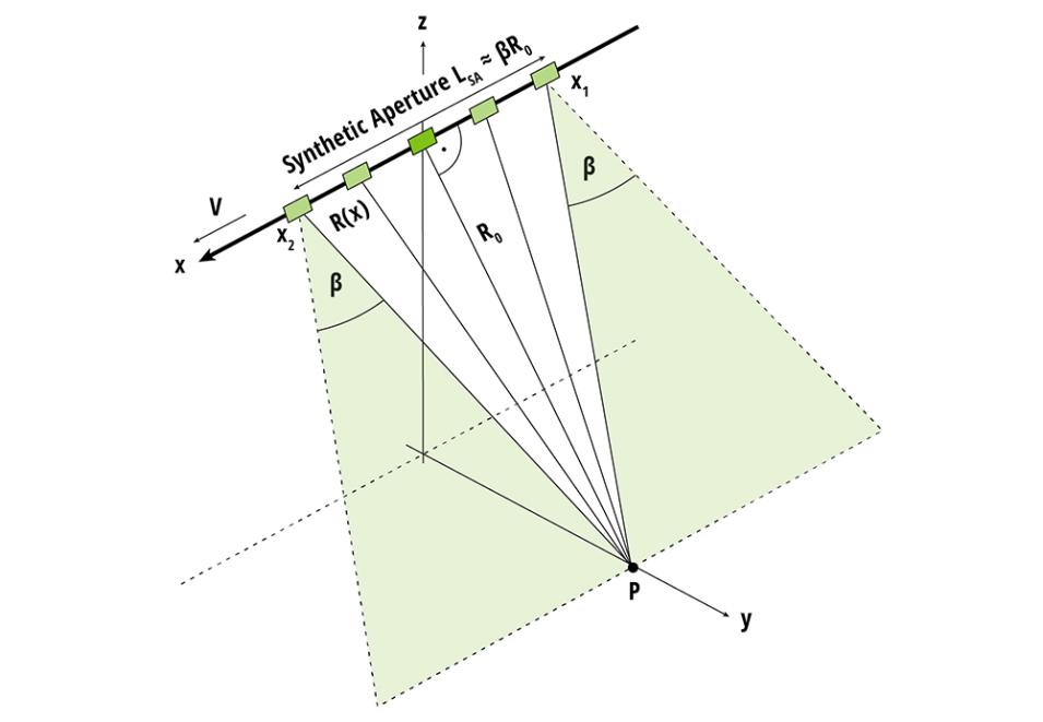
Fig. 5 Schematic of observation geometry used to form a SAR image.
Credit: NASA EarthData / NASA SAR Handbook.

SAR data is collected in slant range, which is the viewing geometry of the side-looking sensor and has two dimensions: range and azimuth. These are the along-track and across-track directions of the imaged swath. As data is transformed from radar coordinates (slant range) to geocoded coordinates, the spaces represented by individual pixels in the two coordinate systems do not always align, and distortions can arise due to certain viewing angle geometries and surface topography features. In addition, radiometric distortion can arise due to scattering responses from multiple scattering features within a single pixel. Radiometric terrain correction is a processing step that accounts for these distortions and the transformation from radar to geocoded coordinates that prepares SAR data for analysis.

Sentinel-1 RTC datasets

Alaska Satellite Facility

Dataset name	Producer	Storage format	Storage location
Sentinel-1 RTC	Alaska Satellite Facility	COG (locally as GeoTIFF)	Local

We use Sentinel-1 RTC imagery processed by Alaska Satellite Facility’s Hybrid Pluggable Processing Pipeline (HyP3) [23]. This is a processing platform that allows users to perform processing steps necessary for analysis-ready SAR data through ASF.

From the ASF HyP3 Documentation: HyP3 is a service for processing Synthetic Aperture Radar (SAR) imagery that addresses many common issues for users of SAR data:

• Most SAR datasets require at least some processing to remove distortions before they are analysis-ready

• SAR processing is computing-intensive

• Software for SAR processing is complicated to use and/or prohibitively expensive

• Producing analysis-ready SAR data has a steep learning curve that acts as a barrier to entry

HyP3 solves these problems by providing a free service where people can request SAR processing on-demand. These processing requests are picked up by automated systems, which handle the complexity of SAR processing on behalf of the user. HyP3 doesn’t require users to have a lot of knowledge of SAR processing before getting started; users only need to submit the input data and set a few optional parameters if desired. With HyP3, analysis-ready products are just a few clicks away.

The data in this tutorial was processed using HyP3 [26] and then published via Zenodo here. For more on how to use HyP3 for your own data processing needs, check out their tutorials page.

Microsoft Planetary Computer

Dataset name	Producer	Storage format	Storage location
Sentinel-1 RTC	Microsoft Planetary Computer	Cloud-optimized GeoTIFF (COG)	Microsoft Azure

In contrast to ASF’s HyP3 SAR data processing service, Microsoft Planetary Computer hosts an already-processed global Sentinel-1 RTC dataset, which we will use in this tutorial. Read more about Planetary Computer’s Sentinel-1 RTC product here.

Further reading on SAR data and Sentinel-1:

• ESA Sentinel-1 documentation

• ASF Introduction to SAR

• NASA Earth Observation Data Basics - SAR

• University of Alaska Fairbanks - Microwave Remote Sensing

• Mathematical tutorial on SAR [8], publicly available via NASA EarthData

Vector data

Randolph Glacier Inventory version 7 (RGI7) glacier outlines

Dataset name	Producer	Storage format	Storage location
Randolph Glacier Inventory	RGI Consortium	Shapefile	NSIDC

The Randolph Glacier Inventory (RGI) is a community-driven public dataset that provides outlines and auxiliary information such as area, length and aspect of glaciers across the world [43]. RGI is a subset of the Global Land Ice Measurements from Space (GLIMS) initiative and RGI data is hosted by the National Snow and Ice Data Center (NSIDC). Read more about the RGI project here.

RGI data used in this tutorial

The link above brings you to the NSIDC data access point for all RGI data. The examples in this tutorial focus areas of interest in High Mountain Asia. We have made available the subset of RGI data covering only these regions that is used in the tutorials in case users would like to use that instead. It is stored as a GeoParquet file in the repository associated with these tutorials.