3.3 Handling raster and vector data

Introduction

In the previous notebook, we worked through challenges that can be associated with working with larger-than-memory datasets. Here, we’ll start where we left off, with a dataset that is organized in chronological order, and has a chunking strategy applied.

So far, we’ve been looking at ice velocity data generated for vast spatial footprints. What we’re actually interested in is how ice velocity varies within and across individual glaciers. To look at this more closely, we’ll use glacier outlines the Randolph Glacier Inventory to subset the velocity data. Once we’ve done this, we can start to ask questions like how does velocity vary over time and across different seasons, where on the glacier do velocities tend to be fastest and most seasonally active, and how do these patterns vary across different glaciers? The last two notebooks of this tutorial will start to address these questions.

In this notebook, we introduce vector data that describes spatial features that we’re interested in. This notebook will:

• Look at how to parse and inspect important geographic metadata.

• Project data to match the coordinate reference system (CRS) of another data object.

• Join raster and vector data by clipping the raster data cube by the spatial extent of a vector data frame.

• Write this clipped raster object to disk.

---

Outline

A. Read data using strategy identified in previous notebook

B. Incorporate glacier outline (vector) data

• 1. Read and reproject vector data

• 2. Visualize spatial extents of glacier outlines and ITS_LIVE data cube

• 3. Crop vector data to spatial extent of raster data

C. Combine raster and vector data

• 1. Use vector data to crop raster data

• 2. Write clipped raster data cube to disk

Learning Goals

Concepts

• Understand how to parse and manage coordinate reference system metadata,

• Visualize vector dataframes with static and interactive plots,

• Spatial subsetting and clipping with vector and raster data,

• Write raster data to disk.

Techniques

• Use cf_xarray and pyproj to access geographic metadata,

• Perform spatial subset of vector dataframe with GeoPandas,

• Clip raster data using vector data with rioxarray.

---

Expand the next cell to see specific packages used in this notebook and relevant system and version information.

Show code cell source Hide code cell source

import cf_xarray
import folium
import geopandas as gpd
import matplotlib.pyplot as plt
import pathlib
import pyproj

import itslive_tools

---

A. Read data using strategy identified in previous notebook

Because we will be reading and writing files to disk, create a variable to hold the path to the root directory for this tutorial; we’ll use this later on.

cwd = pathlib.Path.cwd()
tutorial1_dir = pathlib.Path(cwd).parent

# Find url
url = itslive_tools.find_granule_by_point([95.180191, 30.645973])
# Read data cube without Dask
dc = itslive_tools.read_in_s3(url, chunks=None)
# Sort by mid-date
dc = dc.sortby("mid_date")
# Visually check mid-date in chronological order
dc.mid_date

<xarray.DataArray 'mid_date' (mid_date: 47892)> Size: 383kB
array(['1986-09-11T03:31:15.003252992', '1986-10-05T03:31:06.144750016',
       '1986-10-21T03:31:34.493249984', ..., '2024-10-29T04:18:09.241024000',
       '2024-10-29T04:18:09.241024000', '2024-10-29T04:18:09.241024000'],
      dtype='datetime64[ns]')
Coordinates:
    mapping   <U1 4B ...
  * mid_date  (mid_date) datetime64[ns] 383kB 1986-09-11T03:31:15.003252992 ....
Attributes:
    description:    midpoint of image 1 and image 2 acquisition date and time...
    standard_name:  image_pair_center_date_with_time_separation

xarray.DataArray

'mid_date'

• mid_date: 47892

• 1986-09-11T03:31:15.003252992 ... 2024-10-29T04:18:09.241024

  array(['1986-09-11T03:31:15.003252992', '1986-10-05T03:31:06.144750016',
         '1986-10-21T03:31:34.493249984', ..., '2024-10-29T04:18:09.241024000',
         '2024-10-29T04:18:09.241024000', '2024-10-29T04:18:09.241024000'],
        dtype='datetime64[ns]')

• Coordinates: (2)
  • mapping
    ()
    <U1
    ...

    GeoTransform :

    700072.5 120.0 0 3399967.5 0 -120.0

    crs_wkt :

    PROJCS["WGS 84 / UTM zone 46N",GEOGCS["WGS 84",DATUM["WGS_1984",SPHEROID["WGS 84",6378137,298.257223563,AUTHORITY["EPSG","7030"]],AUTHORITY["EPSG","6326"]],PRIMEM["Greenwich",0,AUTHORITY["EPSG","8901"]],UNIT["degree",0.0174532925199433,AUTHORITY["EPSG","9122"]],AUTHORITY["EPSG","4326"]],PROJECTION["Transverse_Mercator"],PARAMETER["latitude_of_origin",0],PARAMETER["central_meridian",93],PARAMETER["scale_factor",0.9996],PARAMETER["false_easting",500000],PARAMETER["false_northing",0],UNIT["metre",1,AUTHORITY["EPSG","9001"]],AXIS["Easting",EAST],AXIS["Northing",NORTH],AUTHORITY["EPSG","32646"]]

    false_easting :

    500000.0

    false_northing :

    0.0

    grid_mapping_name :

    universal_transverse_mercator

    inverse_flattening :

    298.257223563

    latitude_of_projection_origin :

    0.0

    longitude_of_central_meridian :

    93.0

    proj4text :

    +proj=utm +zone=46 +datum=WGS84 +units=m +no_defs

    scale_factor_at_central_meridian :

    0.9996

    semi_major_axis :

    6378137.0

    spatial_epsg :

    32646

    spatial_ref :

    PROJCS["WGS 84 / UTM zone 46N",GEOGCS["WGS 84",DATUM["WGS_1984",SPHEROID["WGS 84",6378137,298.257223563,AUTHORITY["EPSG","7030"]],AUTHORITY["EPSG","6326"]],PRIMEM["Greenwich",0,AUTHORITY["EPSG","8901"]],UNIT["degree",0.0174532925199433,AUTHORITY["EPSG","9122"]],AUTHORITY["EPSG","4326"]],PROJECTION["Transverse_Mercator"],PARAMETER["latitude_of_origin",0],PARAMETER["central_meridian",93],PARAMETER["scale_factor",0.9996],PARAMETER["false_easting",500000],PARAMETER["false_northing",0],UNIT["metre",1,AUTHORITY["EPSG","9001"]],AXIS["Easting",EAST],AXIS["Northing",NORTH],AUTHORITY["EPSG","32646"]]

    utm_zone_number :

    46.0

    [1 values with dtype=<U1]

  • mid_date
    (mid_date)
    datetime64[ns]
    1986-09-11T03:31:15.003252992 .....

    description :

    midpoint of image 1 and image 2 acquisition date and time with granule's centroid longitude and latitude as microseconds

    standard_name :

    image_pair_center_date_with_time_separation

    array(['1986-09-11T03:31:15.003252992', '1986-10-05T03:31:06.144750016',
           '1986-10-21T03:31:34.493249984', ..., '2024-10-29T04:18:09.241024000',
           '2024-10-29T04:18:09.241024000', '2024-10-29T04:18:09.241024000'],
          dtype='datetime64[ns]')

• Indexes: (1)
  • mid_date
    PandasIndex

    PandasIndex(DatetimeIndex(['1986-09-11 03:31:15.003252992',
                   '1986-10-05 03:31:06.144750016',
                   '1986-10-21 03:31:34.493249984',
                   '1986-11-22 03:29:27.023556992',
                   '1986-11-30 03:29:08.710132992',
                   '1986-12-08 03:29:55.372057024',
                   '1986-12-08 03:33:17.095283968',
                      '1986-12-16 03:30:10.645544',
                   '1986-12-24 03:29:52.332120960',
                   '1987-01-09 03:30:01.787228992',
                   ...
                   '2024-10-21 16:17:50.241008896',
                   '2024-10-24 04:17:34.241014016',
                   '2024-10-24 04:17:34.241014016',
                   '2024-10-24 04:17:34.241014016',
                   '2024-10-24 04:17:34.241014016',
                   '2024-10-25 04:10:35.189837056',
                      '2024-10-29 04:18:09.241024',
                      '2024-10-29 04:18:09.241024',
                      '2024-10-29 04:18:09.241024',
                      '2024-10-29 04:18:09.241024'],
                  dtype='datetime64[ns]', name='mid_date', length=47892, freq=None))

• Attributes: (2)

  description :

  midpoint of image 1 and image 2 acquisition date and time with granule's centroid longitude and latitude as microseconds

  standard_name :

  image_pair_center_date_with_time_separation

Like in the last notebook, we want to chunk the dataset and to do that, we need to assign chunk sizes for each dimension:

chunking_dict = {"mid_date": 20000, "y": 10, "x": 10}

dc = dc.chunk(chunking_dict)

dc.chunks

Frozen({'mid_date': (20000, 20000, 7892), 'y': (10, 10, 10, 10, 10, 10, 10, 10, 10, 10, 10, 10, 10, 10, 10, 10, 10, 10, 10, 10, 10, 10, 10, 10, 10, 10, 10, 10, 10, 10, 10, 10, 10, 10, 10, 10, 10, 10, 10, 10, 10, 10, 10, 10, 10, 10, 10, 10, 10, 10, 10, 10, 10, 10, 10, 10, 10, 10, 10, 10, 10, 10, 10, 10, 10, 10, 10, 10, 10, 10, 10, 10, 10, 10, 10, 10, 10, 10, 10, 10, 10, 10, 10, 3), 'x': (10, 10, 10, 10, 10, 10, 10, 10, 10, 10, 10, 10, 10, 10, 10, 10, 10, 10, 10, 10, 10, 10, 10, 10, 10, 10, 10, 10, 10, 10, 10, 10, 10, 10, 10, 10, 10, 10, 10, 10, 10, 10, 10, 10, 10, 10, 10, 10, 10, 10, 10, 10, 10, 10, 10, 10, 10, 10, 10, 10, 10, 10, 10, 10, 10, 10, 10, 10, 10, 10, 10, 10, 10, 10, 10, 10, 10, 10, 10, 10, 10, 10, 10, 3)})

Looks good 👍

B. Incorporate glacier outline (vector) data

1) Read and reproject vector data

As discussed in the vector data section of the ‘Tutorial Data’ page, the examples in this tutorial use glacier outlines from the Randolph Glacier Inventory], version 7 (RGI7). We’ll specifically be looking at the ‘South Asia East’ region.

se_asia = gpd.read_parquet("../data/vector_data/rgi7_region15_south_asia_east.parquet")

It is vital to check the CRS, or Coordinate Reference Systems, when combining geospatial data from different sources.

The RGI data are in the EPSG:4326 CRS.

se_asia.crs

<Geographic 2D CRS: EPSG:4326>
Name: WGS 84
Axis Info [ellipsoidal]:
- Lat[north]: Geodetic latitude (degree)
- Lon[east]: Geodetic longitude (degree)
Area of Use:
- name: World.
- bounds: (-180.0, -90.0, 180.0, 90.0)
Datum: World Geodetic System 1984 ensemble
- Ellipsoid: WGS 84
- Prime Meridian: Greenwich

The CRS information for the ITS_LIVE dataset is stored in the mapping array. An easy way to discover this is to use the cf_xarray package and search for the grid_mapping variable if present.

dc.cf

Coordinates:
             CF Axes: * X: ['x']
                      * Y: ['y']
                        Z, T: n/a

      CF Coordinates:   longitude, latitude, vertical, time: n/a

       Cell Measures:   area, volume: n/a

      Standard Names: * image_pair_center_date_with_time_separation: ['mid_date']
                      * projection_x_coordinate: ['x']
                      * projection_y_coordinate: ['y']

              Bounds:   n/a

       Grid Mappings:   universal_transverse_mercator: ['mapping']

Data Variables:
       Cell Measures:   area, volume: n/a

      Standard Names:   M11_dr_to_vr_factor: ['M11_dr_to_vr_factor']
                        M12_dr_to_vr_factor: ['M12_dr_to_vr_factor']
                        autoRIFT_software_version: ['autoRIFT_software_version']
                        chip_size_height: ['chip_size_height']
                        chip_size_width: ['chip_size_width']
                        conversion_matrix_element_11: ['M11']
                        conversion_matrix_element_12: ['M12']
                        floating ice mask: ['floatingice']
                        granule_url: ['granule_url']
                        image1_acquition_date: ['acquisition_date_img1']
                        image1_mission: ['mission_img1']
                        image1_satellite: ['satellite_img1']
                        image1_sensor: ['sensor_img1']
                        image2_acquition_date: ['acquisition_date_img2']
                        image2_mission: ['mission_img2']
                        image2_satellite: ['satellite_img2']
                        image2_sensor: ['sensor_img2']
                        image_pair_center_date: ['date_center']
                        image_pair_time_separation: ['date_dt']
                        interpolated_value_mask: ['interp_mask']
                        land ice mask: ['landice']
                        land_ice_surface_velocity: ['v']
                        land_ice_surface_x_velocity: ['vx']
                        land_ice_surface_y_velocity: ['vy']
                        region_of_interest_valid_pixel_percentage: ['roi_valid_percentage']
                        stable_count_slow: ['stable_count_slow']
                        stable_count_stationary: ['stable_count_stationary']
                        stable_shift_flag: ['stable_shift_flag']
                        va_error: ['va_error']
                        va_error_modeled: ['va_error_modeled']
                        va_error_slow: ['va_error_slow']
                        va_error_stationary: ['va_error_stationary']
                        va_stable_shift: ['va_stable_shift']
                        va_stable_shift_slow: ['va_stable_shift_slow']
                        va_stable_shift_stationary: ['va_stable_shift_stationary']
                        velocity_error: ['v_error']
                        vr_error: ['vr_error']
                        vr_error_modeled: ['vr_error_modeled']
                        vr_error_slow: ['vr_error_slow']
                        vr_error_stationary: ['vr_error_stationary']
                        vr_stable_shift: ['vr_stable_shift']
                        vr_stable_shift_slow: ['vr_stable_shift_slow']
                        vr_stable_shift_stationary: ['vr_stable_shift_stationary']
                        vx_error: ['vx_error']
                        vx_error_modeled: ['vx_error_modeled']
                        vx_error_slow: ['vx_error_slow']
                        vx_error_stationary: ['vx_error_stationary']
                        vx_stable_shift: ['vx_stable_shift']
                        vx_stable_shift_slow: ['vx_stable_shift_slow']
                        vx_stable_shift_stationary: ['vx_stable_shift_stationary']
                        vy_error: ['vy_error']
                        vy_error_modeled: ['vy_error_modeled']
                        vy_error_slow: ['vy_error_slow']
                        vy_error_stationary: ['vy_error_stationary']
                        vy_stable_shift: ['vy_stable_shift']
                        vy_stable_shift_slow: ['vy_stable_shift_slow']
                        vy_stable_shift_stationary: ['vy_stable_shift_stationary']

              Bounds:   n/a

       Grid Mappings:   n/a

cube_crs = pyproj.CRS.from_cf(dc.mapping.attrs)
cube_crs

<Projected CRS: EPSG:32646>
Name: WGS 84 / UTM zone 46N
Axis Info [cartesian]:
- [east]: Easting (metre)
- [north]: Northing (metre)
Area of Use:
- undefined
Coordinate Operation:
- name: UTM zone 46N
- method: Transverse Mercator
Datum: World Geodetic System 1984
- Ellipsoid: WGS 84
- Prime Meridian: Greenwich

This indicates that the data is projected to UTM zone 46N (EPSG:32646).

We choose to reproject the glacier outline to the CRS of the datacube:

# Project rgi data to match itslive
se_asia_prj = se_asia.to_crs(cube_crs)
se_asia_prj.head(3)

	rgi_id	o1region	o2region	glims_id	anlys_id	subm_id	src_date	cenlon	cenlat	utm_zone	...	zmin_m	zmax_m	zmed_m	zmean_m	slope_deg	aspect_deg	aspect_sec	dem_source	lmax_m	geometry
0	RGI2000-v7.0-G-15-00001	15	15-01	G078088E31398N	866850	752	2002-07-10T00:00:00	78.087891	31.398046	44	...	4662.2950	4699.2095	4669.4720	4671.4253	13.427070	122.267290	4	COPDEM30	173	POLYGON Z ((-924868.476 3571663.111 0.000, -92...
1	RGI2000-v7.0-G-15-00002	15	15-01	G078125E31399N	867227	752	2002-07-10T00:00:00	78.123699	31.397796	44	...	4453.3584	4705.9920	4570.9473	4571.2770	22.822983	269.669144	7	COPDEM30	1113	POLYGON Z ((-921270.161 3571706.471 0.000, -92...
2	RGI2000-v7.0-G-15-00003	15	15-01	G078128E31390N	867273	752	2000-08-05T00:00:00	78.128510	31.390287	44	...	4791.7593	4858.6807	4832.1836	4827.6700	15.626262	212.719681	6	COPDEM30	327	POLYGON Z ((-921061.745 3570342.665 0.000, -92...

3 rows × 29 columns

How many glaciers are represented in the dataset?

len(se_asia_prj)

18587

2) Visualize spatial extents of glacier outlines and ITS_LIVE data cube

In Accessing S3 Data, we defined a function to create a vector object describing the footprint of a raster object; we’ll use that again here.

# Get vector bbox of itslive
bbox_dc = itslive_tools.get_bounds_polygon(dc)
bbox_dc["geometry"]
# Check that all objects have correct crs
assert dc.attrs["projection"] == bbox_dc.crs == se_asia_prj.crs

# Plot the outline of the itslive granule and the rgi dataframe together
fig, ax = plt.subplots()

bbox_dc.plot(ax=ax, facecolor="None", color="red")
se_asia_prj.plot(ax=ax, facecolor="None")

<Axes: >

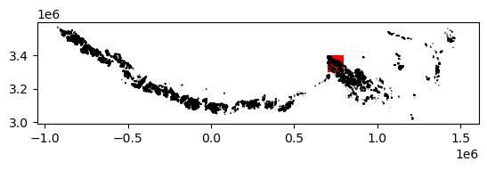
3) Crop vector data to spatial extent of raster data

The above plot shows the coverage of the vector dataset (se_asia_prj) in black, relative to the extent of the raster dataset (bbox_dc) in red. We use the geopandas .clip() method to subset the RGI polygons to the footprint of the ITS_LIVE datacube.

# Subset rgi to bounds
se_asia_subset = gpd.clip(se_asia_prj, bbox_dc)
se_asia_subset.head()

	rgi_id	o1region	o2region	glims_id	anlys_id	subm_id	src_date	cenlon	cenlat	utm_zone	...	zmin_m	zmax_m	zmed_m	zmean_m	slope_deg	aspect_deg	aspect_sec	dem_source	lmax_m	geometry
16373	RGI2000-v7.0-G-15-16374	15	15-03	G095930E29817N	930178	752	2005-09-08T00:00:00	95.929916	29.817003	46	...	4985.7314	5274.0435	5142.7660	5148.8170	27.024134	139.048110	4	COPDEM30	756	POLYGON Z ((783110.719 3302487.481 0.000, 7831...
16374	RGI2000-v7.0-G-15-16375	15	15-03	G095925E29818N	930160	752	2005-09-08T00:00:00	95.925181	29.818399	46	...	4856.2790	5054.9253	4929.5560	4933.6890	44.126980	211.518448	6	COPDEM30	366	POLYGON Z ((782511.360 3302381.154 0.000, 7825...
16376	RGI2000-v7.0-G-15-16377	15	15-03	G095915E29820N	930107	752	2005-09-08T00:00:00	95.914583	29.819510	46	...	5072.8910	5150.6196	5108.5020	5111.7217	23.980000	219.341537	6	COPDEM30	170	POLYGON Z ((781619.822 3302305.074 0.000, 7816...
16371	RGI2000-v7.0-G-15-16372	15	15-03	G095936E29819N	930215	752	2005-09-08T00:00:00	95.935554	29.819123	46	...	4838.7646	5194.8840	5001.5117	4992.3706	25.684517	128.737870	4	COPDEM30	931	POLYGON Z ((783420.055 3302493.804 0.000, 7834...
15879	RGI2000-v7.0-G-15-15880	15	15-03	G095459E29807N	928789	752	1999-07-29T00:00:00	95.459374	29.807181	46	...	3802.1846	4155.1255	4000.2695	4000.4404	28.155806	116.148640	4	COPDEM30	776	POLYGON Z ((737667.211 3300277.169 0.000, 7377...

5 rows × 29 columns

We can use the geopandas .explore() method to interactively look at the RGI7 outlines contained within the ITS_LIVE granule:

m = folium.Map(max_lat=31, max_lon=95, min_lat=29, min_lon=97, location=[30.2, 95.5], zoom_start=8)

bbox_dc.explore(
    m=m,
    style_kwds={"fillColor": "None", "color": "red"},
    legend_kwds={"labels": ["ITS_LIVE granule footprint"]},
)
se_asia_subset.explore(m=m)

folium.LayerControl().add_to(m)
m

/home/emmamarshall/miniforge3/envs/geospatial_datacube_book_env/lib/python3.11/site-packages/folium/features.py:1102: UserWarning: GeoJsonTooltip is not configured to render for GeoJson GeometryCollection geometries. Please consider reworking these features: [{'rgi_id': 'RGI2000-v7.0-G-15-16433', 'o1region': '15', 'o2region': '15-03', 'glims_id': 'G095721E29941N', 'anlys_id': 929520, 'subm_id': 752, 'src_date': '2005-09-08T00:00:00', 'cenlon': 95.7211016152286, 'cenlat': 29.940902187781784, 'utm_zone': 46, 'area_km2': 0.340954350813452, 'primeclass': 0, 'conn_lvl': 0, 'surge_type': 0, 'term_type': 9, 'glac_name': None, 'is_rgi6': 0, 'termlon': 95.72222864596793, 'termlat': 29.937137080413784, 'zmin_m': 4657.792, 'zmax_m': 5049.5625, 'zmed_m': 4825.1104, 'zmean_m': 4839.4185, 'slope_deg': 23.704372, 'aspect_deg': 145.20973, 'aspect_sec': 4, 'dem_source': 'COPDEM30', 'lmax_m': 891}, {'rgi_id': 'RGI2000-v7.0-G-15-12194', 'o1region': '15', 'o2region': '15-03', 'glims_id': 'G095869E30315N', 'anlys_id': 929951, 'subm_id': 752, 'src_date': '2005-09-08T00:00:00', 'cenlon': 95.86889789565677, 'cenlat': 30.3147685, 'utm_zone': 46, 'area_km2': 8.797406997273084, 'primeclass': 0, 'conn_lvl': 0, 'surge_type': 0, 'term_type': 9, 'glac_name': None, 'is_rgi6': 0, 'termlon': 95.89518363763428, 'termlat': 30.307036248571297, 'zmin_m': 4642.1445, 'zmax_m': 5278.752, 'zmed_m': 5011.06, 'zmean_m': 4993.9243, 'slope_deg': 12.372513, 'aspect_deg': 81.418945, 'aspect_sec': 3, 'dem_source': 'COPDEM30', 'lmax_m': 4994}, {'rgi_id': 'RGI2000-v7.0-G-15-11941', 'o1region': '15', 'o2region': '15-03', 'glims_id': 'G095301E30377N', 'anlys_id': 928228, 'subm_id': 752, 'src_date': '2007-08-20T00:00:00', 'cenlon': 95.30071978915663, 'cenlat': 30.3770025, 'utm_zone': 46, 'area_km2': 0.267701958906151, 'primeclass': 0, 'conn_lvl': 0, 'surge_type': 0, 'term_type': 9, 'glac_name': None, 'is_rgi6': 0, 'termlon': 95.30345982475616, 'termlat': 30.380097687364806, 'zmin_m': 5475.784, 'zmax_m': 5977.979, 'zmed_m': 5750.727, 'zmean_m': 5759.621, 'slope_deg': 41.069595, 'aspect_deg': 350.3331518173218, 'aspect_sec': 1, 'dem_source': 'COPDEM30', 'lmax_m': 807}] to MultiPolygon for full functionality.
https://tools.ietf.org/html/rfc7946#page-9
  warnings.warn(

Make this Notebook Trusted to load map: File -> Trust Notebook

We can use the above interactive map to select a glacier to look at in more detail below.

However, notice that while the above code correctly produces a plot, it also throws a warning. We’re going to ignore the warning for now, but if you’re interested in a detailed example of how to trouble shoot and resolve this type of warning, check out the appendix

We write bbox_dc to file so that we can use it in the appendix

bbox_dc.to_file("../data/vector_data/bbox_dc.geojson")

C. Combine raster and vector data

1) Use vector data to crop raster data

If we want to dig in and analyze this velocity dataset at smaller spatial scales, we first need to subset it. The following section and the next notebook (Exploratory data analysis of a single glacier) will focus on the spatial scale of a single glacier.

The glacier we’ll focus on is in the southeastern region of Tibetan Plateau in the Hengduan mountain range. It was selected in part because it is large enough that we should be able to observe velocity variability within the context of the spatial resolution of the ITS_LIVE dataset but is not so large that it is an extreme outlier for glaciers in the region.

# Select a  glacier to subset to
single_glacier_vec = se_asia_subset.loc[se_asia_subset["rgi_id"] == "RGI2000-v7.0-G-15-16257"]
single_glacier_vec

	rgi_id	o1region	o2region	glims_id	anlys_id	subm_id	src_date	cenlon	cenlat	utm_zone	...	zmin_m	zmax_m	zmed_m	zmean_m	slope_deg	aspect_deg	aspect_sec	dem_source	lmax_m	geometry
16256	RGI2000-v7.0-G-15-16257	15	15-03	G095962E29920N	930314	752	2005-09-08T00:00:00	95.961972	29.920094	46	...	4320.7065	5937.84	5179.605	5131.8877	22.803406	100.811325	3	COPDEM30	5958	POLYGON Z ((788176.951 3315860.842 0.000, 7882...

1 rows × 29 columns

# Write it to file to that it can be used later
single_glacier_vec.to_file("../data/single_glacier_vec.json", driver="GeoJSON")

Check to see if the ITS_LIVE raster dataset has an assigned CRS attribute. We already know that the data is projected in the correct coordinate reference system (CRS), but the object may not be ‘CRS-aware’ yet (ie. have an attribute specifying its CRS). This is necessary for spatial operations such as clipping and reprojection. If dc doesn’t have a CRS attribute, use rio.write_crs() to assign it. For more detail, see Rioxarray’s CRS Management documentation.

dc.rio.crs

CRS.from_epsg(32646)

Now, use the subset vector data object and Rioxarray’s .clip() method to crop the data cube.

%%time

single_glacier_raster = dc.rio.clip(single_glacier_vec.geometry, single_glacier_vec.crs)

CPU times: user 2.03 s, sys: 72.4 ms, total: 2.1 s
Wall time: 2.1 s

2) Write clipped raster data cube to disk

We want to use single_glacier_raster in the following notebook without going through all of the steps of creating it again. So, we write the object to file as a Zarr data cube so that we can easily read it into memory when we need it next. However, we’ll see that there are a few steps we must go through before we can successfully write this object.

We first re-chunk the single_glacier_raster into more optimal chunk sizes:

single_glacier_raster = single_glacier_raster.chunk({"mid_date": 20000, "x": 10, "y": 10})
single_glacier_raster

<xarray.Dataset> Size: 3GB
Dimensions:                     (mid_date: 47892, x: 40, y: 37)
Coordinates:
  * mid_date                    (mid_date) datetime64[ns] 383kB 1986-09-11T03...
  * x                           (x) float64 320B 7.843e+05 ... 7.889e+05
  * y                           (y) float64 296B 3.316e+06 ... 3.311e+06
    spatial_ref                 int64 8B 0
    mapping                     int64 8B 0
Data variables: (12/59)
    M11                         (mid_date, y, x) float32 284MB dask.array<chunksize=(20000, 10, 10), meta=np.ndarray>
    M11_dr_to_vr_factor         (mid_date) float32 192kB dask.array<chunksize=(20000,), meta=np.ndarray>
    M12                         (mid_date, y, x) float32 284MB dask.array<chunksize=(20000, 10, 10), meta=np.ndarray>
    M12_dr_to_vr_factor         (mid_date) float32 192kB dask.array<chunksize=(20000,), meta=np.ndarray>
    acquisition_date_img1       (mid_date) datetime64[ns] 383kB dask.array<chunksize=(20000,), meta=np.ndarray>
    acquisition_date_img2       (mid_date) datetime64[ns] 383kB dask.array<chunksize=(20000,), meta=np.ndarray>
    ...                          ...
    vy_error_modeled            (mid_date) float32 192kB dask.array<chunksize=(20000,), meta=np.ndarray>
    vy_error_slow               (mid_date) float32 192kB dask.array<chunksize=(20000,), meta=np.ndarray>
    vy_error_stationary         (mid_date) float32 192kB dask.array<chunksize=(20000,), meta=np.ndarray>
    vy_stable_shift             (mid_date) float32 192kB dask.array<chunksize=(20000,), meta=np.ndarray>
    vy_stable_shift_slow        (mid_date) float32 192kB dask.array<chunksize=(20000,), meta=np.ndarray>
    vy_stable_shift_stationary  (mid_date) float32 192kB dask.array<chunksize=(20000,), meta=np.ndarray>
Attributes: (12/19)
    Conventions:                CF-1.8
    GDAL_AREA_OR_POINT:         Area
    author:                     ITS_LIVE, a NASA MEaSUREs project (its-live.j...
    autoRIFT_parameter_file:    http://its-live-data.s3.amazonaws.com/autorif...
    datacube_software_version:  1.0
    date_created:               25-Sep-2023 22:00:23
    ...                         ...
    s3:                         s3://its-live-data/datacubes/v2/N30E090/ITS_L...
    skipped_granules:           s3://its-live-data/datacubes/v2/N30E090/ITS_L...
    time_standard_img1:         UTC
    time_standard_img2:         UTC
    title:                      ITS_LIVE datacube of image pair velocities
    url:                        https://its-live-data.s3.amazonaws.com/datacu...

xarray.Dataset

• Dimensions:
  • mid_date: 47892
  • x: 40
  • y: 37
• Coordinates: (5)
  • mid_date
    (mid_date)
    datetime64[ns]
    1986-09-11T03:31:15.003252992 .....

    description :

    midpoint of image 1 and image 2 acquisition date and time with granule's centroid longitude and latitude as microseconds

    standard_name :

    image_pair_center_date_with_time_separation

    array(['1986-09-11T03:31:15.003252992', '1986-10-05T03:31:06.144750016',
           '1986-10-21T03:31:34.493249984', ..., '2024-10-29T04:18:09.241024000',
           '2024-10-29T04:18:09.241024000', '2024-10-29T04:18:09.241024000'],
          dtype='datetime64[ns]')

  • x
    (x)
    float64
    7.843e+05 7.844e+05 ... 7.889e+05

    description :

    x coordinate of projection

    standard_name :

    projection_x_coordinate

    axis :

    X

    long_name :

    x coordinate of projection

    units :

    metre

    array([784252.5, 784372.5, 784492.5, 784612.5, 784732.5, 784852.5, 784972.5,
           785092.5, 785212.5, 785332.5, 785452.5, 785572.5, 785692.5, 785812.5,
           785932.5, 786052.5, 786172.5, 786292.5, 786412.5, 786532.5, 786652.5,
           786772.5, 786892.5, 787012.5, 787132.5, 787252.5, 787372.5, 787492.5,
           787612.5, 787732.5, 787852.5, 787972.5, 788092.5, 788212.5, 788332.5,
           788452.5, 788572.5, 788692.5, 788812.5, 788932.5])

  • y
    (y)
    float64
    3.316e+06 3.316e+06 ... 3.311e+06

    description :

    y coordinate of projection

    standard_name :

    projection_y_coordinate

    axis :

    Y

    long_name :

    y coordinate of projection

    units :

    metre

    array([3315787.5, 3315667.5, 3315547.5, 3315427.5, 3315307.5, 3315187.5,
           3315067.5, 3314947.5, 3314827.5, 3314707.5, 3314587.5, 3314467.5,
           3314347.5, 3314227.5, 3314107.5, 3313987.5, 3313867.5, 3313747.5,
           3313627.5, 3313507.5, 3313387.5, 3313267.5, 3313147.5, 3313027.5,
           3312907.5, 3312787.5, 3312667.5, 3312547.5, 3312427.5, 3312307.5,
           3312187.5, 3312067.5, 3311947.5, 3311827.5, 3311707.5, 3311587.5,
           3311467.5])

  • spatial_ref
    ()
    int64
    0

    GeoTransform :

    784192.5 120.0 0.0 3315847.5 0.0 -120.0

    array(0)

  • mapping
    ()
    int64
    0

    crs_wkt :

    PROJCS["WGS 84 / UTM zone 46N",GEOGCS["WGS 84",DATUM["WGS_1984",SPHEROID["WGS 84",6378137,298.257223563,AUTHORITY["EPSG","7030"]],AUTHORITY["EPSG","6326"]],PRIMEM["Greenwich",0,AUTHORITY["EPSG","8901"]],UNIT["degree",0.0174532925199433,AUTHORITY["EPSG","9122"]],AUTHORITY["EPSG","4326"]],PROJECTION["Transverse_Mercator"],PARAMETER["latitude_of_origin",0],PARAMETER["central_meridian",93],PARAMETER["scale_factor",0.9996],PARAMETER["false_easting",500000],PARAMETER["false_northing",0],UNIT["metre",1,AUTHORITY["EPSG","9001"]],AXIS["Easting",EAST],AXIS["Northing",NORTH],AUTHORITY["EPSG","32646"]]

    semi_major_axis :

    6378137.0

    semi_minor_axis :

    6356752.314245179

    inverse_flattening :

    298.257223563

    reference_ellipsoid_name :

    WGS 84

    longitude_of_prime_meridian :

    0.0

    prime_meridian_name :

    Greenwich

    geographic_crs_name :

    WGS 84

    horizontal_datum_name :

    World Geodetic System 1984

    projected_crs_name :

    WGS 84 / UTM zone 46N

    grid_mapping_name :

    transverse_mercator

    latitude_of_projection_origin :

    0.0

    longitude_of_central_meridian :

    93.0

    false_easting :

    500000.0

    false_northing :

    0.0

    scale_factor_at_central_meridian :

    0.9996

    spatial_ref :

    PROJCS["WGS 84 / UTM zone 46N",GEOGCS["WGS 84",DATUM["WGS_1984",SPHEROID["WGS 84",6378137,298.257223563,AUTHORITY["EPSG","7030"]],AUTHORITY["EPSG","6326"]],PRIMEM["Greenwich",0,AUTHORITY["EPSG","8901"]],UNIT["degree",0.0174532925199433,AUTHORITY["EPSG","9122"]],AUTHORITY["EPSG","4326"]],PROJECTION["Transverse_Mercator"],PARAMETER["latitude_of_origin",0],PARAMETER["central_meridian",93],PARAMETER["scale_factor",0.9996],PARAMETER["false_easting",500000],PARAMETER["false_northing",0],UNIT["metre",1,AUTHORITY["EPSG","9001"]],AXIS["Easting",EAST],AXIS["Northing",NORTH],AUTHORITY["EPSG","32646"]]

    GeoTransform :

    784192.5 120.0 0.0 3315847.5 0.0 -120.0

    array(0)

• Data variables: (59)
  • M11
    (mid_date, y, x)
    float32
    dask.array<chunksize=(20000, 10, 10), meta=np.ndarray>

    description :

    conversion matrix element (1st row, 1st column) that can be multiplied with vx to give range pixel displacement dr (see Eq. A18 in https://www.mdpi.com/2072-4292/13/4/749)

    standard_name :

    conversion_matrix_element_11

    units :

    pixel/(meter/year)

    Array Chunk Bytes 270.39 MiB 7.63 MiB Shape (47892, 37, 40) (20000, 10, 10) Dask graph 48 chunks in 7 graph layers Data type float32 numpy.ndarray

  • M11_dr_to_vr_factor
    (mid_date)
    float32
    dask.array<chunksize=(20000,), meta=np.ndarray>

    description :

    multiplicative factor that converts slant range pixel displacement dr to slant range velocity vr

    standard_name :

    M11_dr_to_vr_factor

    units :

    meter/(year*pixel)

    Array Chunk Bytes 187.08 kiB 78.12 kiB Shape (47892,) (20000,) Dask graph 3 chunks in 2 graph layers Data type float32 numpy.ndarray

  • M12
    (mid_date, y, x)
    float32
    dask.array<chunksize=(20000, 10, 10), meta=np.ndarray>

    description :

    conversion matrix element (1st row, 2nd column) that can be multiplied with vy to give range pixel displacement dr (see Eq. A18 in https://www.mdpi.com/2072-4292/13/4/749)

    standard_name :

    conversion_matrix_element_12

    units :

    pixel/(meter/year)

    Array Chunk Bytes 270.39 MiB 7.63 MiB Shape (47892, 37, 40) (20000, 10, 10) Dask graph 48 chunks in 7 graph layers Data type float32 numpy.ndarray

  • M12_dr_to_vr_factor
    (mid_date)
    float32
    dask.array<chunksize=(20000,), meta=np.ndarray>

    description :

    multiplicative factor that converts slant range pixel displacement dr to slant range velocity vr

    standard_name :

    M12_dr_to_vr_factor

    units :

    meter/(year*pixel)

    Array Chunk Bytes 187.08 kiB 78.12 kiB Shape (47892,) (20000,) Dask graph 3 chunks in 2 graph layers Data type float32 numpy.ndarray

  • acquisition_date_img1
    (mid_date)
    datetime64[ns]
    dask.array<chunksize=(20000,), meta=np.ndarray>

    description :

    acquisition date and time of image 1

    standard_name :

    image1_acquition_date

    Array Chunk Bytes 374.16 kiB 156.25 kiB Shape (47892,) (20000,) Dask graph 3 chunks in 2 graph layers Data type datetime64[ns] numpy.ndarray

  • acquisition_date_img2
    (mid_date)
    datetime64[ns]
    dask.array<chunksize=(20000,), meta=np.ndarray>

    description :

    acquisition date and time of image 2

    standard_name :

    image2_acquition_date

    Array Chunk Bytes 374.16 kiB 156.25 kiB Shape (47892,) (20000,) Dask graph 3 chunks in 2 graph layers Data type datetime64[ns] numpy.ndarray

  • autoRIFT_software_version
    (mid_date)
    <U5
    dask.array<chunksize=(20000,), meta=np.ndarray>

    description :

    version of autoRIFT software

    standard_name :

    autoRIFT_software_version

    Array Chunk Bytes 0.91 MiB 390.62 kiB Shape (47892,) (20000,) Dask graph 3 chunks in 2 graph layers Data type

  • chip_size_height
    (mid_date, y, x)
    float32
    dask.array<chunksize=(20000, 10, 10), meta=np.ndarray>

    chip_size_coordinates :

    Optical data: chip_size_coordinates = 'image projection geometry: width = x, height = y'. Radar data: chip_size_coordinates = 'radar geometry: width = range, height = azimuth'

    description :

    height of search template (chip)

    standard_name :

    chip_size_height

    units :

    m

    y_pixel_size :

    10.0

    Array Chunk Bytes 270.39 MiB 7.63 MiB Shape (47892, 37, 40) (20000, 10, 10) Dask graph 48 chunks in 7 graph layers Data type float32 numpy.ndarray

  • chip_size_width
    (mid_date, y, x)
    float32
    dask.array<chunksize=(20000, 10, 10), meta=np.ndarray>

    chip_size_coordinates :

    Optical data: chip_size_coordinates = 'image projection geometry: width = x, height = y'. Radar data: chip_size_coordinates = 'radar geometry: width = range, height = azimuth'

    description :

    width of search template (chip)

    standard_name :

    chip_size_width

    units :

    m

    x_pixel_size :

    10.0

    Array Chunk Bytes 270.39 MiB 7.63 MiB Shape (47892, 37, 40) (20000, 10, 10) Dask graph 48 chunks in 7 graph layers Data type float32 numpy.ndarray

  • date_center
    (mid_date)
    datetime64[ns]
    dask.array<chunksize=(20000,), meta=np.ndarray>

    description :

    midpoint of image 1 and image 2 acquisition date

    standard_name :

    image_pair_center_date

    Array Chunk Bytes 374.16 kiB 156.25 kiB Shape (47892,) (20000,) Dask graph 3 chunks in 2 graph layers Data type datetime64[ns] numpy.ndarray

  • date_dt
    (mid_date)
    float32
    dask.array<chunksize=(20000,), meta=np.ndarray>

    description :

    time separation between acquisition of image 1 and image 2

    standard_name :

    image_pair_time_separation

    units :

    days

    Array Chunk Bytes 187.08 kiB 78.12 kiB Shape (47892,) (20000,) Dask graph 3 chunks in 2 graph layers Data type float32 numpy.ndarray

  • floatingice
    (y, x)
    float32
    dask.array<chunksize=(10, 10), meta=np.ndarray>

    description :

    floating ice mask, 0 = non-floating-ice, 1 = floating-ice

    flag_meanings :

    non-ice ice

    flag_values :

    [0, 1]

    standard_name :

    floating ice mask

    url :

    https://its-live-data.s3.amazonaws.com/autorift_parameters/v001/N46_0120m_floatingice.tif

    Array Chunk Bytes 5.78 kiB 400 B Shape (37, 40) (10, 10) Dask graph 16 chunks in 7 graph layers Data type float32 numpy.ndarray

  • granule_url
    (mid_date)
    <U1024
    dask.array<chunksize=(20000,), meta=np.ndarray>

    description :

    original granule URL

    standard_name :

    granule_url

    Array Chunk Bytes 187.08 MiB 78.12 MiB Shape (47892,) (20000,) Dask graph 3 chunks in 2 graph layers Data type

  • interp_mask
    (mid_date, y, x)
    float32
    dask.array<chunksize=(20000, 10, 10), meta=np.ndarray>

    description :

    light interpolation mask

    flag_meanings :

    measured interpolated

    flag_values :

    [0, 1]

    standard_name :

    interpolated_value_mask

    Array Chunk Bytes 270.39 MiB 7.63 MiB Shape (47892, 37, 40) (20000, 10, 10) Dask graph 48 chunks in 7 graph layers Data type float32 numpy.ndarray

  • landice
    (y, x)
    float32
    dask.array<chunksize=(10, 10), meta=np.ndarray>

    description :

    land ice mask, 0 = non-land-ice, 1 = land-ice

    flag_meanings :

    non-ice ice

    flag_values :

    [0, 1]

    standard_name :

    land ice mask

    url :

    https://its-live-data.s3.amazonaws.com/autorift_parameters/v001/N46_0120m_landice.tif

    Array Chunk Bytes 5.78 kiB 400 B Shape (37, 40) (10, 10) Dask graph 16 chunks in 7 graph layers Data type float32 numpy.ndarray

  • mission_img1
    (mid_date)
    <U1
    dask.array<chunksize=(20000,), meta=np.ndarray>

    description :

    id of the mission that acquired image 1

    standard_name :

    image1_mission

    Array Chunk Bytes 187.08 kiB 78.12 kiB Shape (47892,) (20000,) Dask graph 3 chunks in 2 graph layers Data type

  • mission_img2
    (mid_date)
    <U1
    dask.array<chunksize=(20000,), meta=np.ndarray>

    description :

    id of the mission that acquired image 2

    standard_name :

    image2_mission

    Array Chunk Bytes 187.08 kiB 78.12 kiB Shape (47892,) (20000,) Dask graph 3 chunks in 2 graph layers Data type

  • roi_valid_percentage
    (mid_date)
    float32
    dask.array<chunksize=(20000,), meta=np.ndarray>

    description :

    percentage of pixels with a valid velocity estimate determined for the intersection of the full image pair footprint and the region of interest (roi) that defines where autoRIFT tried to estimate a velocity

    standard_name :

    region_of_interest_valid_pixel_percentage

    Array Chunk Bytes 187.08 kiB 78.12 kiB Shape (47892,) (20000,) Dask graph 3 chunks in 2 graph layers Data type float32 numpy.ndarray

  • satellite_img1
    (mid_date)
    <U2
    dask.array<chunksize=(20000,), meta=np.ndarray>

    description :

    id of the satellite that acquired image 1

    standard_name :

    image1_satellite

    Array Chunk Bytes 374.16 kiB 156.25 kiB Shape (47892,) (20000,) Dask graph 3 chunks in 2 graph layers Data type

  • satellite_img2
    (mid_date)
    <U2
    dask.array<chunksize=(20000,), meta=np.ndarray>

    description :

    id of the satellite that acquired image 2

    standard_name :

    image2_satellite

    Array Chunk Bytes 374.16 kiB 156.25 kiB Shape (47892,) (20000,) Dask graph 3 chunks in 2 graph layers Data type

  • sensor_img1
    (mid_date)
    <U3
    dask.array<chunksize=(20000,), meta=np.ndarray>

    description :

    id of the sensor that acquired image 1

    standard_name :

    image1_sensor

    Array Chunk Bytes 561.23 kiB 234.38 kiB Shape (47892,) (20000,) Dask graph 3 chunks in 2 graph layers Data type

  • sensor_img2
    (mid_date)
    <U3
    dask.array<chunksize=(20000,), meta=np.ndarray>

    description :

    id of the sensor that acquired image 2

    standard_name :

    image2_sensor

    Array Chunk Bytes 561.23 kiB 234.38 kiB Shape (47892,) (20000,) Dask graph 3 chunks in 2 graph layers Data type

  • stable_count_slow
    (mid_date)
    uint16
    dask.array<chunksize=(20000,), meta=np.ndarray>

    description :

    number of valid pixels over slowest 25% of ice

    standard_name :

    stable_count_slow

    units :

    count

    Array Chunk Bytes 93.54 kiB 39.06 kiB Shape (47892,) (20000,) Dask graph 3 chunks in 2 graph layers Data type uint16 numpy.ndarray

  • stable_count_stationary
    (mid_date)
    uint16
    dask.array<chunksize=(20000,), meta=np.ndarray>

    description :

    number of valid pixels over stationary or slow-flowing surfaces

    standard_name :

    stable_count_stationary

    units :

    count

    Array Chunk Bytes 93.54 kiB 39.06 kiB Shape (47892,) (20000,) Dask graph 3 chunks in 2 graph layers Data type uint16 numpy.ndarray

  • stable_shift_flag
    (mid_date)
    uint8
    dask.array<chunksize=(20000,), meta=np.ndarray>

    description :

    flag for applying velocity bias correction: 0 = no correction; 1 = correction from overlapping stable surface mask (stationary or slow-flowing surfaces with velocity < 15 m/yr)(top priority); 2 = correction from slowest 25% of overlapping velocities (second priority)

    standard_name :

    stable_shift_flag

    Array Chunk Bytes 46.77 kiB 19.53 kiB Shape (47892,) (20000,) Dask graph 3 chunks in 2 graph layers Data type uint8 numpy.ndarray

  • v
    (mid_date, y, x)
    float32
    dask.array<chunksize=(20000, 10, 10), meta=np.ndarray>

    description :

    velocity magnitude

    standard_name :

    land_ice_surface_velocity

    units :

    meter/year

    Array Chunk Bytes 270.39 MiB 7.63 MiB Shape (47892, 37, 40) (20000, 10, 10) Dask graph 48 chunks in 7 graph layers Data type float32 numpy.ndarray

  • v_error
    (mid_date, y, x)
    float32
    dask.array<chunksize=(20000, 10, 10), meta=np.ndarray>

    description :

    velocity magnitude error

    standard_name :

    velocity_error

    units :

    meter/year

    Array Chunk Bytes 270.39 MiB 7.63 MiB Shape (47892, 37, 40) (20000, 10, 10) Dask graph 48 chunks in 7 graph layers Data type float32 numpy.ndarray

  • va
    (mid_date, y, x)
    float32
    dask.array<chunksize=(20000, 10, 10), meta=np.ndarray>

    description :

    velocity in radar azimuth direction

    Array Chunk Bytes 270.39 MiB 7.63 MiB Shape (47892, 37, 40) (20000, 10, 10) Dask graph 48 chunks in 7 graph layers Data type float32 numpy.ndarray

  • va_error
    (mid_date)
    float32
    dask.array<chunksize=(20000,), meta=np.ndarray>

    description :

    error for velocity in radar azimuth direction

    standard_name :

    va_error

    units :

    meter/year

    Array Chunk Bytes 187.08 kiB 78.12 kiB Shape (47892,) (20000,) Dask graph 3 chunks in 2 graph layers Data type float32 numpy.ndarray

  • va_error_modeled
    (mid_date)
    float32
    dask.array<chunksize=(20000,), meta=np.ndarray>

    description :

    1-sigma error calculated using a modeled error-dt relationship

    standard_name :

    va_error_modeled

    units :

    meter/year

    Array Chunk Bytes 187.08 kiB 78.12 kiB Shape (47892,) (20000,) Dask graph 3 chunks in 2 graph layers Data type float32 numpy.ndarray

  • va_error_slow
    (mid_date)
    float32
    dask.array<chunksize=(20000,), meta=np.ndarray>

    description :

    RMSE over slowest 25% of retrieved velocities

    standard_name :

    va_error_slow

    units :

    meter/year

    Array Chunk Bytes 187.08 kiB 78.12 kiB Shape (47892,) (20000,) Dask graph 3 chunks in 2 graph layers Data type float32 numpy.ndarray

  • va_error_stationary
    (mid_date)
    float32
    dask.array<chunksize=(20000,), meta=np.ndarray>

    description :

    RMSE over stable surfaces, stationary or slow-flowing surfaces with velocity < 15 m/yr identified from an external mask

    standard_name :

    va_error_stationary

    units :

    meter/year

    Array Chunk Bytes 187.08 kiB 78.12 kiB Shape (47892,) (20000,) Dask graph 3 chunks in 2 graph layers Data type float32 numpy.ndarray

  • va_stable_shift
    (mid_date)
    float32
    dask.array<chunksize=(20000,), meta=np.ndarray>

    description :

    applied va shift calibrated using pixels over stable or slow surfaces

    standard_name :

    va_stable_shift

    units :

    meter/year

    Array Chunk Bytes 187.08 kiB 78.12 kiB Shape (47892,) (20000,) Dask graph 3 chunks in 2 graph layers Data type float32 numpy.ndarray

  • va_stable_shift_slow
    (mid_date)
    float32
    dask.array<chunksize=(20000,), meta=np.ndarray>

    description :

    va shift calibrated using valid pixels over slowest 25% of retrieved velocities

    standard_name :

    va_stable_shift_slow

    units :

    meter/year

    Array Chunk Bytes 187.08 kiB 78.12 kiB Shape (47892,) (20000,) Dask graph 3 chunks in 2 graph layers Data type float32 numpy.ndarray

  • va_stable_shift_stationary
    (mid_date)
    float32
    dask.array<chunksize=(20000,), meta=np.ndarray>

    description :

    va shift calibrated using valid pixels over stable surfaces, stationary or slow-flowing surfaces with velocity < 15 m/yr identified from an external mask

    standard_name :

    va_stable_shift_stationary

    units :

    meter/year

    Array Chunk Bytes 187.08 kiB 78.12 kiB Shape (47892,) (20000,) Dask graph 3 chunks in 2 graph layers Data type float32 numpy.ndarray

  • vr
    (mid_date, y, x)
    float32
    dask.array<chunksize=(20000, 10, 10), meta=np.ndarray>

    description :

    velocity in radar range direction

    Array Chunk Bytes 270.39 MiB 7.63 MiB Shape (47892, 37, 40) (20000, 10, 10) Dask graph 48 chunks in 7 graph layers Data type float32 numpy.ndarray

  • vr_error
    (mid_date)
    float32
    dask.array<chunksize=(20000,), meta=np.ndarray>

    description :

    error for velocity in radar range direction

    standard_name :

    vr_error

    units :

    meter/year

    Array Chunk Bytes 187.08 kiB 78.12 kiB Shape (47892,) (20000,) Dask graph 3 chunks in 2 graph layers Data type float32 numpy.ndarray

  • vr_error_modeled
    (mid_date)
    float32
    dask.array<chunksize=(20000,), meta=np.ndarray>

    description :

    1-sigma error calculated using a modeled error-dt relationship

    standard_name :

    vr_error_modeled

    units :

    meter/year

    Array Chunk Bytes 187.08 kiB 78.12 kiB Shape (47892,) (20000,) Dask graph 3 chunks in 2 graph layers Data type float32 numpy.ndarray

  • vr_error_slow
    (mid_date)
    float32
    dask.array<chunksize=(20000,), meta=np.ndarray>

    description :

    RMSE over slowest 25% of retrieved velocities

    standard_name :

    vr_error_slow

    units :

    meter/year

    Array Chunk Bytes 187.08 kiB 78.12 kiB Shape (47892,) (20000,) Dask graph 3 chunks in 2 graph layers Data type float32 numpy.ndarray

  • vr_error_stationary
    (mid_date)
    float32
    dask.array<chunksize=(20000,), meta=np.ndarray>

    description :

    RMSE over stable surfaces, stationary or slow-flowing surfaces with velocity < 15 m/yr identified from an external mask

    standard_name :

    vr_error_stationary

    units :

    meter/year

    Array Chunk Bytes 187.08 kiB 78.12 kiB Shape (47892,) (20000,) Dask graph 3 chunks in 2 graph layers Data type float32 numpy.ndarray

  • vr_stable_shift
    (mid_date)
    float32
    dask.array<chunksize=(20000,), meta=np.ndarray>

    description :

    applied vr shift calibrated using pixels over stable or slow surfaces

    standard_name :

    vr_stable_shift

    units :

    meter/year

    Array Chunk Bytes 187.08 kiB 78.12 kiB Shape (47892,) (20000,) Dask graph 3 chunks in 2 graph layers Data type float32 numpy.ndarray

  • vr_stable_shift_slow
    (mid_date)
    float32
    dask.array<chunksize=(20000,), meta=np.ndarray>

    description :

    vr shift calibrated using valid pixels over slowest 25% of retrieved velocities

    standard_name :

    vr_stable_shift_slow

    units :

    meter/year

    Array Chunk Bytes 187.08 kiB 78.12 kiB Shape (47892,) (20000,) Dask graph 3 chunks in 2 graph layers Data type float32 numpy.ndarray

  • vr_stable_shift_stationary
    (mid_date)
    float32
    dask.array<chunksize=(20000,), meta=np.ndarray>

    description :

    vr shift calibrated using valid pixels over stable surfaces, stationary or slow-flowing surfaces with velocity < 15 m/yr identified from an external mask

    standard_name :

    vr_stable_shift_stationary

    units :

    meter/year

    Array Chunk Bytes 187.08 kiB 78.12 kiB Shape (47892,) (20000,) Dask graph 3 chunks in 2 graph layers Data type float32 numpy.ndarray

  • vx
    (mid_date, y, x)
    float32
    dask.array<chunksize=(20000, 10, 10), meta=np.ndarray>

    description :

    velocity component in x direction

    standard_name :

    land_ice_surface_x_velocity

    units :

    meter/year

    Array Chunk Bytes 270.39 MiB 7.63 MiB Shape (47892, 37, 40) (20000, 10, 10) Dask graph 48 chunks in 7 graph layers Data type float32 numpy.ndarray

  • vx_error
    (mid_date)
    float32
    dask.array<chunksize=(20000,), meta=np.ndarray>

    description :

    best estimate of x_velocity error: vx_error is populated according to the approach used for the velocity bias correction as indicated in "stable_shift_flag"

    standard_name :

    vx_error

    units :

    meter/year

    Array Chunk Bytes 187.08 kiB 78.12 kiB Shape (47892,) (20000,) Dask graph 3 chunks in 2 graph layers Data type float32 numpy.ndarray

  • vx_error_modeled
    (mid_date)
    float32
    dask.array<chunksize=(20000,), meta=np.ndarray>

    description :

    1-sigma error calculated using a modeled error-dt relationship

    standard_name :

    vx_error_modeled

    units :

    meter/year

    Array Chunk Bytes 187.08 kiB 78.12 kiB Shape (47892,) (20000,) Dask graph 3 chunks in 2 graph layers Data type float32 numpy.ndarray

  • vx_error_slow
    (mid_date)
    float32
    dask.array<chunksize=(20000,), meta=np.ndarray>

    description :

    RMSE over slowest 25% of retrieved velocities

    standard_name :

    vx_error_slow

    units :

    meter/year

    Array Chunk Bytes 187.08 kiB 78.12 kiB Shape (47892,) (20000,) Dask graph 3 chunks in 2 graph layers Data type float32 numpy.ndarray

  • vx_error_stationary
    (mid_date)
    float32
    dask.array<chunksize=(20000,), meta=np.ndarray>

    description :

    RMSE over stable surfaces, stationary or slow-flowing surfaces with velocity < 15 meter/year identified from an external mask

    standard_name :

    vx_error_stationary

    units :

    meter/year

    Array Chunk Bytes 187.08 kiB 78.12 kiB Shape (47892,) (20000,) Dask graph 3 chunks in 2 graph layers Data type float32 numpy.ndarray

  • vx_stable_shift
    (mid_date)
    float32
    dask.array<chunksize=(20000,), meta=np.ndarray>

    description :

    applied vx shift calibrated using pixels over stable or slow surfaces

    standard_name :

    vx_stable_shift

    units :

    meter/year

    Array Chunk Bytes 187.08 kiB 78.12 kiB Shape (47892,) (20000,) Dask graph 3 chunks in 2 graph layers Data type float32 numpy.ndarray

  • vx_stable_shift_slow
    (mid_date)
    float32
    dask.array<chunksize=(20000,), meta=np.ndarray>

    description :

    vx shift calibrated using valid pixels over slowest 25% of retrieved velocities

    standard_name :

    vx_stable_shift_slow

    units :

    meter/year

    Array Chunk Bytes 187.08 kiB 78.12 kiB Shape (47892,) (20000,) Dask graph 3 chunks in 2 graph layers Data type float32 numpy.ndarray

  • vx_stable_shift_stationary
    (mid_date)
    float32
    dask.array<chunksize=(20000,), meta=np.ndarray>

    description :

    vx shift calibrated using valid pixels over stable surfaces, stationary or slow-flowing surfaces with velocity < 15 m/yr identified from an external mask

    standard_name :

    vx_stable_shift_stationary

    units :

    meter/year

    Array Chunk Bytes 187.08 kiB 78.12 kiB Shape (47892,) (20000,) Dask graph 3 chunks in 2 graph layers Data type float32 numpy.ndarray

  • vy
    (mid_date, y, x)
    float32
    dask.array<chunksize=(20000, 10, 10), meta=np.ndarray>

    description :

    velocity component in y direction

    standard_name :

    land_ice_surface_y_velocity

    units :

    meter/year

    Array Chunk Bytes 270.39 MiB 7.63 MiB Shape (47892, 37, 40) (20000, 10, 10) Dask graph 48 chunks in 7 graph layers Data type float32 numpy.ndarray

  • vy_error
    (mid_date)
    float32
    dask.array<chunksize=(20000,), meta=np.ndarray>

    description :

    best estimate of y_velocity error: vy_error is populated according to the approach used for the velocity bias correction as indicated in "stable_shift_flag"

    standard_name :

    vy_error

    units :

    meter/year

    Array Chunk Bytes 187.08 kiB 78.12 kiB Shape (47892,) (20000,) Dask graph 3 chunks in 2 graph layers Data type float32 numpy.ndarray

  • vy_error_modeled
    (mid_date)
    float32
    dask.array<chunksize=(20000,), meta=np.ndarray>

    description :

    1-sigma error calculated using a modeled error-dt relationship

    standard_name :

    vy_error_modeled

    units :

    meter/year

    Array Chunk Bytes 187.08 kiB 78.12 kiB Shape (47892,) (20000,) Dask graph 3 chunks in 2 graph layers Data type float32 numpy.ndarray

  • vy_error_slow
    (mid_date)
    float32
    dask.array<chunksize=(20000,), meta=np.ndarray>

    description :

    RMSE over slowest 25% of retrieved velocities

    standard_name :

    vy_error_slow

    units :

    meter/year

    Array Chunk Bytes 187.08 kiB 78.12 kiB Shape (47892,) (20000,) Dask graph 3 chunks in 2 graph layers Data type float32 numpy.ndarray

  • vy_error_stationary
    (mid_date)
    float32
    dask.array<chunksize=(20000,), meta=np.ndarray>

    description :

    RMSE over stable surfaces, stationary or slow-flowing surfaces with velocity < 15 meter/year identified from an external mask

    standard_name :

    vy_error_stationary

    units :

    meter/year

    Array Chunk Bytes 187.08 kiB 78.12 kiB Shape (47892,) (20000,) Dask graph 3 chunks in 2 graph layers Data type float32 numpy.ndarray

  • vy_stable_shift
    (mid_date)
    float32
    dask.array<chunksize=(20000,), meta=np.ndarray>

    description :

    applied vy shift calibrated using pixels over stable or slow surfaces

    standard_name :

    vy_stable_shift

    units :

    meter/year

    Array Chunk Bytes 187.08 kiB 78.12 kiB Shape (47892,) (20000,) Dask graph 3 chunks in 2 graph layers Data type float32 numpy.ndarray

  • vy_stable_shift_slow
    (mid_date)
    float32
    dask.array<chunksize=(20000,), meta=np.ndarray>

    description :

    vy shift calibrated using valid pixels over slowest 25% of retrieved velocities

    standard_name :

    vy_stable_shift_slow

    units :

    meter/year

    Array Chunk Bytes 187.08 kiB 78.12 kiB Shape (47892,) (20000,) Dask graph 3 chunks in 2 graph layers Data type float32 numpy.ndarray

  • vy_stable_shift_stationary
    (mid_date)
    float32
    dask.array<chunksize=(20000,), meta=np.ndarray>

    description :

    vy shift calibrated using valid pixels over stable surfaces, stationary or slow-flowing surfaces with velocity < 15 m/yr identified from an external mask

    standard_name :

    vy_stable_shift_stationary

    units :

    meter/year

    Array Chunk Bytes 187.08 kiB 78.12 kiB Shape (47892,) (20000,) Dask graph 3 chunks in 2 graph layers Data type float32 numpy.ndarray

• Indexes: (3)
  • mid_date
    PandasIndex

    PandasIndex(DatetimeIndex(['1986-09-11 03:31:15.003252992',
                   '1986-10-05 03:31:06.144750016',
                   '1986-10-21 03:31:34.493249984',
                   '1986-11-22 03:29:27.023556992',
                   '1986-11-30 03:29:08.710132992',
                   '1986-12-08 03:29:55.372057024',
                   '1986-12-08 03:33:17.095283968',
                      '1986-12-16 03:30:10.645544',
                   '1986-12-24 03:29:52.332120960',
                   '1987-01-09 03:30:01.787228992',
                   ...
                   '2024-10-21 16:17:50.241008896',
                   '2024-10-24 04:17:34.241014016',
                   '2024-10-24 04:17:34.241014016',
                   '2024-10-24 04:17:34.241014016',
                   '2024-10-24 04:17:34.241014016',
                   '2024-10-25 04:10:35.189837056',
                      '2024-10-29 04:18:09.241024',
                      '2024-10-29 04:18:09.241024',
                      '2024-10-29 04:18:09.241024',
                      '2024-10-29 04:18:09.241024'],
                  dtype='datetime64[ns]', name='mid_date', length=47892, freq=None))

  • x
    PandasIndex

    PandasIndex(Index([784252.5, 784372.5, 784492.5, 784612.5, 784732.5, 784852.5, 784972.5,
           785092.5, 785212.5, 785332.5, 785452.5, 785572.5, 785692.5, 785812.5,
           785932.5, 786052.5, 786172.5, 786292.5, 786412.5, 786532.5, 786652.5,
           786772.5, 786892.5, 787012.5, 787132.5, 787252.5, 787372.5, 787492.5,
           787612.5, 787732.5, 787852.5, 787972.5, 788092.5, 788212.5, 788332.5,
           788452.5, 788572.5, 788692.5, 788812.5, 788932.5],
          dtype='float64', name='x'))

  • y
    PandasIndex

    PandasIndex(Index([3315787.5, 3315667.5, 3315547.5, 3315427.5, 3315307.5, 3315187.5,
           3315067.5, 3314947.5, 3314827.5, 3314707.5, 3314587.5, 3314467.5,
           3314347.5, 3314227.5, 3314107.5, 3313987.5, 3313867.5, 3313747.5,
           3313627.5, 3313507.5, 3313387.5, 3313267.5, 3313147.5, 3313027.5,
           3312907.5, 3312787.5, 3312667.5, 3312547.5, 3312427.5, 3312307.5,
           3312187.5, 3312067.5, 3311947.5, 3311827.5, 3311707.5, 3311587.5,
           3311467.5],
          dtype='float64', name='y'))

• Attributes: (19)

  Conventions :

  CF-1.8

  GDAL_AREA_OR_POINT :

  Area

  author :

  ITS_LIVE, a NASA MEaSUREs project (its-live.jpl.nasa.gov)

  autoRIFT_parameter_file :

  http://its-live-data.s3.amazonaws.com/autorift_parameters/v001/autorift_landice_0120m.shp

  datacube_software_version :

  1.0

  date_created :

  25-Sep-2023 22:00:23

  date_updated :

  13-Nov-2024 00:08:07

  geo_polygon :

  [[95.06959008486952, 29.814255053135895], [95.32812062059084, 29.809951334550703], [95.58659184122865, 29.80514261876954], [95.84499718862224, 29.7998293459177], [96.10333011481168, 29.79401200205343], [96.11032804508507, 30.019297601073085], [96.11740568350054, 30.244573983323825], [96.12456379063154, 30.469841094022847], [96.1318031397002, 30.695098878594504], [95.87110827645229, 30.70112924501256], [95.61033817656023, 30.7066371044805], [95.34949964126946, 30.711621947056347], [95.08859948278467, 30.716083310981194], [95.08376623410525, 30.49063893600811], [95.07898726183609, 30.26518607254204], [95.0742620484426, 30.039724763743482], [95.06959008486952, 29.814255053135895]]

  institution :

  NASA Jet Propulsion Laboratory (JPL), California Institute of Technology

  latitude :

  30.26

  longitude :

  95.6

  proj_polygon :

  [[700000, 3300000], [725000.0, 3300000.0], [750000.0, 3300000.0], [775000.0, 3300000.0], [800000, 3300000], [800000.0, 3325000.0], [800000.0, 3350000.0], [800000.0, 3375000.0], [800000, 3400000], [775000.0, 3400000.0], [750000.0, 3400000.0], [725000.0, 3400000.0], [700000, 3400000], [700000.0, 3375000.0], [700000.0, 3350000.0], [700000.0, 3325000.0], [700000, 3300000]]

  projection :

  32646

  s3 :

  s3://its-live-data/datacubes/v2/N30E090/ITS_LIVE_vel_EPSG32646_G0120_X750000_Y3350000.zarr

  skipped_granules :

  s3://its-live-data/datacubes/v2/N30E090/ITS_LIVE_vel_EPSG32646_G0120_X750000_Y3350000.json

  time_standard_img1 :

  UTC

  time_standard_img2 :

  UTC

  title :

  ITS_LIVE datacube of image pair velocities

  url :

  https://its-live-data.s3.amazonaws.com/datacubes/v2/N30E090/ITS_LIVE_vel_EPSG32646_G0120_X750000_Y3350000.zarr

If we try to write single_glacier_raster, eg:

single_glacier_raster.to_zarr('data/itslive/glacier_itslive.zarr', mode='w')

We’ll received an error related to encoding.

The root cause is that the encoding recorded was appropriate for the source dataset, but is not valid anymore given all the transformations we have run up to this point. The easy solution here is to simply call drop_encoding. This will delete any existing encoding isntructions, and have Xarray automatically choose an encoding that will work well for the data. Optimizing the encoding of on-disk data is an advanced topic that we will not cover.

Now, let’s try to write the object as a Zarr group.

single_glacier_raster.drop_encoding().to_zarr("../data/raster_data/single_glacier_itslive.zarr", mode="w")

<xarray.backends.zarr.ZarrStore at 0x7e73b2be8540>

Conclusion

In this notebook, we read a large object into memory and clipped it to the footprint of a single area of using a large vector dataframe, all the while managing coordinate reference system metadata of both objects. We then saved the clipped raster object to disk so that it can be easily reused. The next notebook demonstrates exploratory data analysis steps using the object we just wrote to disk.