2.6 Relevant concepts#
Larger-than-memory data, parallelization, and Dask#
- Larger than memory data#
Several notebooks in these tutorials discuss ‘larger-than-memory’ datasets and strategies for working with them ‘in memory.’ What does this mean? When we say memory, we refer to the available CPU space or RAM on whatever machine you’re working on. You might also see this called ‘internal memory.’ When working with smaller datasets, the data and intermediate copies created during many operations don’t exceed the internal memory available on our machine. However, as datasets increase in size, the memory required for many workflows can quickly scale and exceed the availability of most personal machines. This is what we mean when we refer to ‘larger than memory’ data. With large datasets, we need to employ different approaches that can be a bit more complicated than a straightforward operation that ingests and produces smaller amounts of data.
- Dask#
There are different ways to approach a dataset that is too large to load into memory. In this tutorial, we rely on the Python library, Dask. Dask allows you to parallelize your workflows, breaking up a large job into many smaller jobs that can be executed in parallel rather than in sequence with one another. Parallelized jobs can be distributed across cores on an individual computer or across large, distributed compute nodes in cloud-computing environments. These tutorials use to parallelize and distribute jobs across one machine. Conveniently, Dask also has built-in integrations with many open-source Python libraries, including Xarray; this means that we can specify and create Dask-backed Xarray objects within Xarray commands such as
xr.open_dataset()rather than needing to create them separately.An important aspect of Dask is that its operations are ‘lazy’ by default: if I have an array (
arr) and I want to perform an operation on it (let’s imagine something very simple, like multiplying the array by 5), when I execute that operation in Python (arr * 5), as long as it is a Dask Array (or an Xarray object backed by Dask Arrays), the computation is not actually executed yet. Dask uses task scheduling to track, orchestrate, and synchronize operations. When I callarr * 5, rather than calculating the resulting product, Dask adds it to a Task Graph. A Task Graph consists of Python functions and the inputs and outputs of those functions; they are used by the program to direct how jobs should be distributed and executed across available resources in order to correctly complete the desired operation.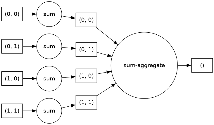
Fig. 6 Image of a task graph associated with applying .sum() to a
xr.DataArray. Source: Project Pythia Dask Cookbook section on Task Graphs.#So what can happen lazily and what can’t? Dask will wait to evaluate a set of operations until it is explicitly instructed to do so. This can be through calling a direct method (like
.compute()or.persist()), or an operation that cannot be accomplished lazily (like plotting an array). For more detail, check out Dask’s Managing Computation documentation.- Chunking#
Dask operates by breaking up large tasks into smaller ones. In our context, this is accomplished mainly through Dask Arrays. If you’re familiar with the Xarray data model, you’ll know that the fundamental building block of a standard Xarray DataArray is a NumPy array; a
Xr.DataArrayis just a NumPy array with named dimensions and coordinates, and separate NumPy arrays describing those coordinates.When we introduce Dask to an Xarray workflow, we convert the underlying
.dataobjects of an Xarray object from NumPy arrays to Dask Arrays. Luckily, Dask arrays aren’t too unfamiliar; a Dask Array is composed of NumPy-like arrays but with an additional specification:chunks. Chunks tell Dask how to break up the array into smaller parts. For example, if you have a 3-dimensional Xarray DataArray, you will specify how the object should be chunked along each dimension.Choosing chunks can be complicated and significantly impact how fast your code runs. Typically, you want enough chunks such that individual chunks are relatively small and many chunks can fit into memory. However, if you have too many chunks, Dask now needs to keep track of many individual tasks, meaning that more time will be spent managing the task graph relative to executing tasks. In addition, tasks should reflect the shape of your data and how you want to use it. If you’re working with a space-time dataset but are most interested in spatial analysis, having smaller chunks along the
xandydimensions will make spatial operations easier to parallelize.Further reading
Choosing good chunk sizes blog post,
Xarray - Parallel Computing with Dask
Specifically the Chunking and Performance section.
Importance of metadata naming and metadata naming conventions#
- Metadata naming#
Metadata is vital to understanding your dataset, however, because of the range of types of metadata and ways it is often stored, it can become very complicated to work with and keep track of. There are a few priorities to keep in mind when working with metadata and/or writing your own.
Metadata should be added to the
attrsof an Xarray object so that the dataset is self-describing (You or a future user don’t need external information to be able to interpret the data).Wherever possible, metadata should follow Climate Forecast (CF) naming conventions.
- Climate Forecast (CF) Metadata Conventions#
CF conventions address many challenges related to inconsistent and non-descriptive metadata found in climate and earth observation datasets. By establishing standard naming schemes for physical quantities and other attributes, these conventions facilitate collaboration, data fusion, and the development of tools for working with a range of data types.
From the CF documentation:
The CF metadata conventions are designed to promote the processing and sharing of files created with the NetCDF API. The conventions define metadata that provide a definitive description of what the data in each variable represents, as well as the spatial and temporal properties of the data. This enables users of data from different sources to decide which quantities are comparable and facilitates building applications with powerful extraction, regridding, and display capabilities. The CF convention includes a standard name table, which defines strings that identify physical quantities.
CF metadata conventions set common expectations for metadata names and locations across datasets. In this tutorial, we will use tools such as cf_xarray that leverage CF conventions to add programmatic handling of CF metadata to Xarray objects, meaning users can spend less time wrangling metadata.
- Spatio-temporal Asset Catalog (STAC)#
STAC is a metadata specification for geospatial data that allows the data to be more easily “worked with, indexed, and discovered”
The STAC specification is built around four core objects: Items, Catalogs, Collections, and an API. These take the form of a series of GeoJSON and JSON files that allow users to lazily query and index datasets before actually reading data into memory, which can be especially helpful for data stored in cloud object storage. Working off of a common metadata structure allows a suite of generalized tools to be developed and used to query and read all sorts of data, as long as they have STAC-compliant metadata. A few examples of these tools are PySTAC, stackstac, and odc-stac. stackstac and odc-stac both provide methods to read STAC data into memory as Xarray Datasets. If you’re interested, see this Pangeo thread for a discussion of the similarities and differences between these approaches.
Further reading