Applied example: RTC time series analysis

Now that we have done so much work to organize these two datasets and prepare them for analysis, let’s explore the data with a scientific question in mind.

In this example, we have data over a specific area of interest covering two glaciers and two proglacial lakes in the Central Himalaya near the India-Chinese border. As a glaciologist, I might be interested in questions related to the conditions of these surface – is there a seasonal pattern to proglacial lake conditions? Do they freeze during the winter, and if so, at similar times? What is the surface of the glacier like at certain times of year? SAR backscatter imagery may not conclusively answer any of these questions in itself, but it can provide important insights about surface conditions and how they change over time that could be used to answer some of these questions.

This notebook will walk through some initial steps of how you could use the data objects we’ve created to explore backscatter dynamics over time and space for the area of interest we have identified.

Learning objectives

Concepts

• Subset larger dataset to spatial areas of interest

• Computations and reductions

• Data visualization

Techniques

• GeoPandas:
  - Handling projections
  - Spatial joins of multiple vector datasets
  - Interactive data visualization

• Xarray and RioXarray:
  - Clip raster object by a vector object
  - Computations and reductions along different dimensions
  - Data visualization

Other useful resources

These are resources that contain additional examples and discussion of the content in this notebook and more.

• Xarray user guide

• How do I… this is very helpful!

• Xarray High-level computational patterns discussion of concepts and associated code examples

• Parallel computing with dask Xarray tutorial demonstrating wrapping of dask arrays

Software and setup

%xmode minimal

Exception reporting mode: Minimal

import geopandas as gpd
import xarray as xr
from shapely import geometry
import matplotlib.pyplot as plt
import numpy as np

Utility functions

def get_bbox_single(input_xr, buffer = 0):
    
    '''Takes input xr object (from itslive data cube), plots a quick map of the footprint. 
    currently only working for granules in crs epsg 32645'''

    xmin = input_xr.coords['x'].data.min()
    xmax = input_xr.coords['x'].data.max()

    ymin = input_xr.coords['y'].data.min()
    ymax = input_xr.coords['y'].data.max()

    pts_ls = [(xmin, ymin), (xmax, ymin),(xmax, ymax), (xmin, ymax), (xmin, ymin)]
 
    crs = input_xr.rio.crs

    polygon_geom = geometry.Polygon(pts_ls)
    polygon = gpd.GeoDataFrame(index=[0], crs=crs, geometry=[polygon_geom]) 
    polygon_prj = polygon
    polygon = polygon_prj.to_crs(crs)

    #add a buffer if needed
    bounds = polygon.total_bounds
    #bounds = [bounds[0]-500, bounds[2]+500, bounds[1]-500, bounds[3]+500]
    
    bounds_xmin = bounds[0]-buffer
    bounds_xmax = bounds[2]+buffer
    bounds_ymin = bounds[1]-buffer
    bounds_ymax = bounds[3]+buffer
    
    bounds_ls = [(bounds_xmin, bounds_ymin), (bounds_xmax, bounds_ymin),
                 (bounds_xmax, bounds_ymax), (bounds_xmin, bounds_ymax),
                 (bounds_xmin, bounds_ymin)]
                   
    
    bounds_geom = geometry.Polygon(bounds_ls)
    bound_gdf = gpd.GeoDataFrame(index=[0], crs=crs, geometry = [bounds_geom])
    bounds_prj = bound_gdf.to_crs(crs)
    
    return bounds_prj

def power_to_db(input_arr):
    return (10*np.log10(np.abs(input_arr)))

Read in prepared RTC data

• this example will use ASF dataset

%store -r vrt_full

vrt_full

<xarray.Dataset>
Dimensions:                           (acq_date: 103, y: 396, x: 290)
Coordinates: (12/17)
  * acq_date                          (acq_date) datetime64[ns] 2021-05-02T12...
  * x                                 (x) float64 6.194e+05 ... 6.281e+05
  * y                                 (y) float64 3.102e+06 ... 3.09e+06
    spatial_ref                       int64 0
    sensor                            (acq_date) <U3 'S1A' 'S1A' ... 'S1A' 'S1A'
    beam_mode                         (acq_date) <U2 'IW' 'IW' ... 'IW' 'IW'
    ...                                ...
    masked                            (acq_date) <U1 'u' 'u' 'u' ... 'u' 'u' 'u'
    filtered                          (acq_date) <U1 'n' 'n' 'n' ... 'n' 'n' 'n'
    area                              (acq_date) <U1 'e' 'e' 'e' ... 'e' 'e' 'e'
    product_id                        (acq_date) <U4 '748F' '0D1E' ... 'BD36'
    granule_id                        (acq_date) <U67 'S1A_IW_SLC__1SDV_20210...
    orbital_dir                       (acq_date) <U4 'desc' 'asc' ... 'desc'
Data variables:
    vv                                (acq_date, y, x) float32 dask.array<chunksize=(1, 396, 290), meta=np.ndarray>
    vh                                (acq_date, y, x) float32 dask.array<chunksize=(1, 396, 290), meta=np.ndarray>
    ls                                (acq_date, y, x) float64 dask.array<chunksize=(1, 396, 290), meta=np.ndarray>

xarray.Dataset

• Dimensions:
  • acq_date: 103
  • y: 396
  • x: 290
• Coordinates: (17)
  • acq_date
    (acq_date)
    datetime64[ns]
    2021-05-02T12:14:14 ... 2022-05-...

    array(['2021-05-02T12:14:14.000000000', '2021-05-05T00:03:07.000000000',
           '2021-05-09T12:05:42.000000000', '2021-05-14T12:13:49.000000000',
           '2021-05-14T12:14:14.000000000', '2021-05-17T00:03:08.000000000',
           '2021-05-21T12:05:43.000000000', '2021-05-26T12:13:50.000000000',
           '2021-05-29T00:03:09.000000000', '2021-06-02T12:05:43.000000000',
           '2021-06-07T12:13:51.000000000', '2021-06-10T00:03:10.000000000',
           '2021-06-14T12:05:44.000000000', '2021-06-19T12:13:52.000000000',
           '2021-06-22T00:03:10.000000000', '2021-06-26T12:05:45.000000000',
           '2021-07-01T12:13:52.000000000', '2021-07-01T12:14:17.000000000',
           '2021-07-04T00:03:11.000000000', '2021-07-08T12:05:45.000000000',
           '2021-07-13T12:13:53.000000000', '2021-07-13T12:14:18.000000000',
           '2021-07-13T12:14:18.000000000', '2021-07-16T00:03:12.000000000',
           '2021-07-20T12:05:46.000000000', '2021-07-25T12:13:54.000000000',
           '2021-07-28T00:03:12.000000000', '2021-08-01T12:05:47.000000000',
           '2021-08-06T12:13:54.000000000', '2021-08-09T00:03:13.000000000',
           '2021-08-13T12:05:48.000000000', '2021-08-18T12:13:55.000000000',
           '2021-08-21T00:03:14.000000000', '2021-08-25T12:05:48.000000000',
           '2021-08-30T12:13:56.000000000', '2021-09-02T00:03:14.000000000',
           '2021-09-06T12:05:49.000000000', '2021-09-11T12:13:56.000000000',
           '2021-09-14T00:03:15.000000000', '2021-09-18T12:05:49.000000000',
           '2021-09-23T12:13:57.000000000', '2021-09-26T00:03:15.000000000',
           '2021-09-30T12:05:50.000000000', '2021-10-05T12:13:57.000000000',
           '2021-10-08T00:03:15.000000000', '2021-10-12T12:05:50.000000000',
           '2021-10-17T12:13:57.000000000', '2021-10-20T00:03:16.000000000',
           '2021-10-24T12:05:50.000000000', '2021-10-29T12:13:57.000000000',
           '2021-11-01T00:03:15.000000000', '2021-11-05T12:05:49.000000000',
           '2021-11-10T12:13:57.000000000', '2021-11-13T00:03:15.000000000',
           '2021-11-17T12:05:49.000000000', '2021-11-22T12:13:56.000000000',
           '2021-11-25T00:03:15.000000000', '2021-11-29T12:05:49.000000000',
           '2021-12-04T12:13:56.000000000', '2021-12-07T00:03:14.000000000',
           '2021-12-11T12:05:48.000000000', '2021-12-16T12:13:55.000000000',
           '2021-12-19T00:03:14.000000000', '2021-12-23T12:05:48.000000000',
           '2021-12-28T12:13:55.000000000', '2021-12-31T00:03:13.000000000',
           '2022-01-04T12:05:47.000000000', '2022-01-09T12:13:54.000000000',
           '2022-01-12T00:03:13.000000000', '2022-01-16T12:05:47.000000000',
           '2022-01-21T12:13:54.000000000', '2022-01-24T00:03:12.000000000',
           '2022-01-28T12:05:46.000000000', '2022-02-02T12:13:53.000000000',
           '2022-02-05T00:03:12.000000000', '2022-02-09T12:05:46.000000000',
           '2022-02-14T12:13:53.000000000', '2022-02-17T00:03:11.000000000',
           '2022-02-21T12:05:46.000000000', '2022-02-26T12:13:53.000000000',
           '2022-03-01T00:03:11.000000000', '2022-03-05T12:05:45.000000000',
           '2022-03-10T12:13:53.000000000', '2022-03-13T00:03:11.000000000',
           '2022-03-17T12:05:45.000000000', '2022-03-22T12:13:53.000000000',
           '2022-03-25T00:03:12.000000000', '2022-03-29T12:05:46.000000000',
           '2022-04-03T12:13:53.000000000', '2022-04-03T12:14:18.000000000',
           '2022-04-06T00:03:12.000000000', '2022-04-10T12:05:46.000000000',
           '2022-04-15T12:13:53.000000000', '2022-04-18T00:03:12.000000000',
           '2022-04-22T12:05:47.000000000', '2022-04-27T12:13:54.000000000',
           '2022-04-30T00:03:13.000000000', '2022-05-04T12:05:47.000000000',
           '2022-05-09T12:13:55.000000000', '2022-05-16T12:05:48.000000000',
           '2022-05-21T12:13:56.000000000', '2022-05-21T12:14:20.000000000',
           '2022-05-21T12:14:20.000000000'], dtype='datetime64[ns]')

  • x
    (x)
    float64
    6.194e+05 6.195e+05 ... 6.281e+05

    axis :

    X

    long_name :

    x coordinate of projection

    standard_name :

    projection_x_coordinate

    units :

    metre

    array([619425., 619455., 619485., ..., 628035., 628065., 628095.])

  • y
    (y)
    float64
    3.102e+06 3.102e+06 ... 3.09e+06

    axis :

    Y

    long_name :

    y coordinate of projection

    standard_name :

    projection_y_coordinate

    units :

    metre

    array([3101655., 3101625., 3101595., ..., 3089865., 3089835., 3089805.])

  • spatial_ref
    ()
    int64
    0

    crs_wkt :

    PROJCS["WGS 84 / UTM zone 45N",GEOGCS["WGS 84",DATUM["WGS_1984",SPHEROID["WGS 84",6378137,298.257223563,AUTHORITY["EPSG","7030"]],AUTHORITY["EPSG","6326"]],PRIMEM["Greenwich",0,AUTHORITY["EPSG","8901"]],UNIT["degree",0.0174532925199433,AUTHORITY["EPSG","9122"]],AUTHORITY["EPSG","4326"]],PROJECTION["Transverse_Mercator"],PARAMETER["latitude_of_origin",0],PARAMETER["central_meridian",87],PARAMETER["scale_factor",0.9996],PARAMETER["false_easting",500000],PARAMETER["false_northing",0],UNIT["metre",1,AUTHORITY["EPSG","9001"]],AXIS["Easting",EAST],AXIS["Northing",NORTH],AUTHORITY["EPSG","32645"]]

    semi_major_axis :

    6378137.0

    semi_minor_axis :

    6356752.314245179

    inverse_flattening :

    298.257223563

    reference_ellipsoid_name :

    WGS 84

    longitude_of_prime_meridian :

    0.0

    prime_meridian_name :

    Greenwich

    geographic_crs_name :

    WGS 84

    horizontal_datum_name :

    World Geodetic System 1984

    projected_crs_name :

    WGS 84 / UTM zone 45N

    grid_mapping_name :

    transverse_mercator

    latitude_of_projection_origin :

    0.0

    longitude_of_central_meridian :

    87.0

    false_easting :

    500000.0

    false_northing :

    0.0

    scale_factor_at_central_meridian :

    0.9996

    spatial_ref :

    PROJCS["WGS 84 / UTM zone 45N",GEOGCS["WGS 84",DATUM["WGS_1984",SPHEROID["WGS 84",6378137,298.257223563,AUTHORITY["EPSG","7030"]],AUTHORITY["EPSG","6326"]],PRIMEM["Greenwich",0,AUTHORITY["EPSG","8901"]],UNIT["degree",0.0174532925199433,AUTHORITY["EPSG","9122"]],AUTHORITY["EPSG","4326"]],PROJECTION["Transverse_Mercator"],PARAMETER["latitude_of_origin",0],PARAMETER["central_meridian",87],PARAMETER["scale_factor",0.9996],PARAMETER["false_easting",500000],PARAMETER["false_northing",0],UNIT["metre",1,AUTHORITY["EPSG","9001"]],AXIS["Easting",EAST],AXIS["Northing",NORTH],AUTHORITY["EPSG","32645"]]

    GeoTransform :

    619410.0 30.0 0.0 3101670.0 0.0 -30.0

    array(0)

  • sensor
    (acq_date)
    <U3
    'S1A' 'S1A' 'S1A' ... 'S1A' 'S1A'

    array(['S1A', 'S1A', 'S1A', 'S1A', 'S1A', 'S1A', 'S1A', 'S1A', 'S1A',
           'S1A', 'S1A', 'S1A', 'S1A', 'S1A', 'S1A', 'S1A', 'S1A', 'S1A',
           'S1A', 'S1A', 'S1A', 'S1A', 'S1A', 'S1A', 'S1A', 'S1A', 'S1A',
           'S1A', 'S1A', 'S1A', 'S1A', 'S1A', 'S1A', 'S1A', 'S1A', 'S1A',
           'S1A', 'S1A', 'S1A', 'S1A', 'S1A', 'S1A', 'S1A', 'S1A', 'S1A',
           'S1A', 'S1A', 'S1A', 'S1A', 'S1A', 'S1A', 'S1A', 'S1A', 'S1A',
           'S1A', 'S1A', 'S1A', 'S1A', 'S1A', 'S1A', 'S1A', 'S1A', 'S1A',
           'S1A', 'S1A', 'S1A', 'S1A', 'S1A', 'S1A', 'S1A', 'S1A', 'S1A',
           'S1A', 'S1A', 'S1A', 'S1A', 'S1A', 'S1A', 'S1A', 'S1A', 'S1A',
           'S1A', 'S1A', 'S1A', 'S1A', 'S1A', 'S1A', 'S1A', 'S1A', 'S1A',
           'S1A', 'S1A', 'S1A', 'S1A', 'S1A', 'S1A', 'S1A', 'S1A', 'S1A',
           'S1A', 'S1A', 'S1A', 'S1A'], dtype='<U3')

  • beam_mode
    (acq_date)
    <U2
    'IW' 'IW' 'IW' ... 'IW' 'IW' 'IW'

    array(['IW', 'IW', 'IW', 'IW', 'IW', 'IW', 'IW', 'IW', 'IW', 'IW', 'IW',
           'IW', 'IW', 'IW', 'IW', 'IW', 'IW', 'IW', 'IW', 'IW', 'IW', 'IW',
           'IW', 'IW', 'IW', 'IW', 'IW', 'IW', 'IW', 'IW', 'IW', 'IW', 'IW',
           'IW', 'IW', 'IW', 'IW', 'IW', 'IW', 'IW', 'IW', 'IW', 'IW', 'IW',
           'IW', 'IW', 'IW', 'IW', 'IW', 'IW', 'IW', 'IW', 'IW', 'IW', 'IW',
           'IW', 'IW', 'IW', 'IW', 'IW', 'IW', 'IW', 'IW', 'IW', 'IW', 'IW',
           'IW', 'IW', 'IW', 'IW', 'IW', 'IW', 'IW', 'IW', 'IW', 'IW', 'IW',
           'IW', 'IW', 'IW', 'IW', 'IW', 'IW', 'IW', 'IW', 'IW', 'IW', 'IW',
           'IW', 'IW', 'IW', 'IW', 'IW', 'IW', 'IW', 'IW', 'IW', 'IW', 'IW',
           'IW', 'IW', 'IW', 'IW'], dtype='<U2')

  • polarisation_type
    (acq_date)
    <U2
    'DV' 'DV' 'DV' ... 'DV' 'DV' 'DV'

    array(['DV', 'DV', 'DV', 'DV', 'DV', 'DV', 'DV', 'DV', 'DV', 'DV', 'DV',
           'DV', 'DV', 'DV', 'DV', 'DV', 'DV', 'DV', 'DV', 'DV', 'DV', 'DV',
           'DV', 'DV', 'DV', 'DV', 'DV', 'DV', 'DV', 'DV', 'DV', 'DV', 'DV',
           'DV', 'DV', 'DV', 'DV', 'DV', 'DV', 'DV', 'DV', 'DV', 'DV', 'DV',
           'DV', 'DV', 'DV', 'DV', 'DV', 'DV', 'DV', 'DV', 'DV', 'DV', 'DV',
           'DV', 'DV', 'DV', 'DV', 'DV', 'DV', 'DV', 'DV', 'DV', 'DV', 'DV',
           'DV', 'DV', 'DV', 'DV', 'DV', 'DV', 'DV', 'DV', 'DV', 'DV', 'DV',
           'DV', 'DV', 'DV', 'DV', 'DV', 'DV', 'DV', 'DV', 'DV', 'DV', 'DV',
           'DV', 'DV', 'DV', 'DV', 'DV', 'DV', 'DV', 'DV', 'DV', 'DV', 'DV',
           'DV', 'DV', 'DV', 'DV'], dtype='<U2')

  • orbit_type
    (acq_date)
    <U1
    '_' '_' '_' '_' ... '_' '_' '_' '_'

    array(['_', '_', '_', '_', '_', '_', '_', '_', '_', '_', '_', '_', '_',
           '_', '_', '_', '_', '_', '_', '_', '_', '_', '_', '_', '_', '_',
           '_', '_', '_', '_', '_', '_', '_', '_', '_', '_', '_', '_', '_',
           '_', '_', '_', '_', '_', '_', '_', '_', '_', '_', '_', '_', '_',
           '_', '_', '_', '_', '_', '_', '_', '_', '_', '_', '_', '_', '_',
           '_', '_', '_', '_', '_', '_', '_', '_', '_', '_', '_', '_', '_',
           '_', '_', '_', '_', '_', '_', '_', '_', '_', '_', '_', '_', '_',
           '_', '_', '_', '_', '_', '_', '_', '_', '_', '_', '_', '_'],
          dtype='<U1')

  • terrain_correction_pixel_spacing
    (acq_date)
    <U5
    'RTC30' 'RTC30' ... 'RTC30' 'RTC30'

    array(['RTC30', 'RTC30', 'RTC30', 'RTC30', 'RTC30', 'RTC30', 'RTC30',
           'RTC30', 'RTC30', 'RTC30', 'RTC30', 'RTC30', 'RTC30', 'RTC30',
           'RTC30', 'RTC30', 'RTC30', 'RTC30', 'RTC30', 'RTC30', 'RTC30',
           'RTC30', 'RTC30', 'RTC30', 'RTC30', 'RTC30', 'RTC30', 'RTC30',
           'RTC30', 'RTC30', 'RTC30', 'RTC30', 'RTC30', 'RTC30', 'RTC30',
           'RTC30', 'RTC30', 'RTC30', 'RTC30', 'RTC30', 'RTC30', 'RTC30',
           'RTC30', 'RTC30', 'RTC30', 'RTC30', 'RTC30', 'RTC30', 'RTC30',
           'RTC30', 'RTC30', 'RTC30', 'RTC30', 'RTC30', 'RTC30', 'RTC30',
           'RTC30', 'RTC30', 'RTC30', 'RTC30', 'RTC30', 'RTC30', 'RTC30',
           'RTC30', 'RTC30', 'RTC30', 'RTC30', 'RTC30', 'RTC30', 'RTC30',
           'RTC30', 'RTC30', 'RTC30', 'RTC30', 'RTC30', 'RTC30', 'RTC30',
           'RTC30', 'RTC30', 'RTC30', 'RTC30', 'RTC30', 'RTC30', 'RTC30',
           'RTC30', 'RTC30', 'RTC30', 'RTC30', 'RTC30', 'RTC30', 'RTC30',
           'RTC30', 'RTC30', 'RTC30', 'RTC30', 'RTC30', 'RTC30', 'RTC30',
           'RTC30', 'RTC30', 'RTC30', 'RTC30', 'RTC30'], dtype='<U5')

  • output_format
    (acq_date)
    <U1
    'g' 'g' 'g' 'g' ... 'g' 'g' 'g' 'g'

    array(['g', 'g', 'g', 'g', 'g', 'g', 'g', 'g', 'g', 'g', 'g', 'g', 'g',
           'g', 'g', 'g', 'g', 'g', 'g', 'g', 'g', 'g', 'g', 'g', 'g', 'g',
           'g', 'g', 'g', 'g', 'g', 'g', 'g', 'g', 'g', 'g', 'g', 'g', 'g',
           'g', 'g', 'g', 'g', 'g', 'g', 'g', 'g', 'g', 'g', 'g', 'g', 'g',
           'g', 'g', 'g', 'g', 'g', 'g', 'g', 'g', 'g', 'g', 'g', 'g', 'g',
           'g', 'g', 'g', 'g', 'g', 'g', 'g', 'g', 'g', 'g', 'g', 'g', 'g',
           'g', 'g', 'g', 'g', 'g', 'g', 'g', 'g', 'g', 'g', 'g', 'g', 'g',
           'g', 'g', 'g', 'g', 'g', 'g', 'g', 'g', 'g', 'g', 'g', 'g'],
          dtype='<U1')

  • output_type
    (acq_date)
    <U1
    'p' 'p' 'p' 'p' ... 'p' 'p' 'p' 'p'

    array(['p', 'p', 'p', 'p', 'p', 'p', 'p', 'p', 'p', 'p', 'p', 'p', 'p',
           'p', 'p', 'p', 'p', 'p', 'p', 'p', 'p', 'p', 'p', 'p', 'p', 'p',
           'p', 'p', 'p', 'p', 'p', 'p', 'p', 'p', 'p', 'p', 'p', 'p', 'p',
           'p', 'p', 'p', 'p', 'p', 'p', 'p', 'p', 'p', 'p', 'p', 'p', 'p',
           'p', 'p', 'p', 'p', 'p', 'p', 'p', 'p', 'p', 'p', 'p', 'p', 'p',
           'p', 'p', 'p', 'p', 'p', 'p', 'p', 'p', 'p', 'p', 'p', 'p', 'p',
           'p', 'p', 'p', 'p', 'p', 'p', 'p', 'p', 'p', 'p', 'p', 'p', 'p',
           'p', 'p', 'p', 'p', 'p', 'p', 'p', 'p', 'p', 'p', 'p', 'p'],
          dtype='<U1')

  • masked
    (acq_date)
    <U1
    'u' 'u' 'u' 'u' ... 'u' 'u' 'u' 'u'

    array(['u', 'u', 'u', 'u', 'u', 'u', 'u', 'u', 'u', 'u', 'u', 'u', 'u',
           'u', 'u', 'u', 'u', 'u', 'u', 'u', 'u', 'u', 'u', 'u', 'u', 'u',
           'u', 'u', 'u', 'u', 'u', 'u', 'u', 'u', 'u', 'u', 'u', 'u', 'u',
           'u', 'u', 'u', 'u', 'u', 'u', 'u', 'u', 'u', 'u', 'u', 'u', 'u',
           'u', 'u', 'u', 'u', 'u', 'u', 'u', 'u', 'u', 'u', 'u', 'u', 'u',
           'u', 'u', 'u', 'u', 'u', 'u', 'u', 'u', 'u', 'u', 'u', 'u', 'u',
           'u', 'u', 'u', 'u', 'u', 'u', 'u', 'u', 'u', 'u', 'u', 'u', 'u',
           'u', 'u', 'u', 'u', 'u', 'u', 'u', 'u', 'u', 'u', 'u', 'u'],
          dtype='<U1')

  • filtered
    (acq_date)
    <U1
    'n' 'n' 'n' 'n' ... 'n' 'n' 'n' 'n'

    array(['n', 'n', 'n', 'n', 'n', 'n', 'n', 'n', 'n', 'n', 'n', 'n', 'n',
           'n', 'n', 'n', 'n', 'n', 'n', 'n', 'n', 'n', 'n', 'n', 'n', 'n',
           'n', 'n', 'n', 'n', 'n', 'n', 'n', 'n', 'n', 'n', 'n', 'n', 'n',
           'n', 'n', 'n', 'n', 'n', 'n', 'n', 'n', 'n', 'n', 'n', 'n', 'n',
           'n', 'n', 'n', 'n', 'n', 'n', 'n', 'n', 'n', 'n', 'n', 'n', 'n',
           'n', 'n', 'n', 'n', 'n', 'n', 'n', 'n', 'n', 'n', 'n', 'n', 'n',
           'n', 'n', 'n', 'n', 'n', 'n', 'n', 'n', 'n', 'n', 'n', 'n', 'n',
           'n', 'n', 'n', 'n', 'n', 'n', 'n', 'n', 'n', 'n', 'n', 'n'],
          dtype='<U1')

  • area
    (acq_date)
    <U1
    'e' 'e' 'e' 'e' ... 'e' 'e' 'e' 'e'

    array(['e', 'e', 'e', 'e', 'e', 'e', 'e', 'e', 'e', 'e', 'e', 'e', 'e',
           'e', 'e', 'e', 'e', 'e', 'e', 'e', 'e', 'e', 'e', 'e', 'e', 'e',
           'e', 'e', 'e', 'e', 'e', 'e', 'e', 'e', 'e', 'e', 'e', 'e', 'e',
           'e', 'e', 'e', 'e', 'e', 'e', 'e', 'e', 'e', 'e', 'e', 'e', 'e',
           'e', 'e', 'e', 'e', 'e', 'e', 'e', 'e', 'e', 'e', 'e', 'e', 'e',
           'e', 'e', 'e', 'e', 'e', 'e', 'e', 'e', 'e', 'e', 'e', 'e', 'e',
           'e', 'e', 'e', 'e', 'e', 'e', 'e', 'e', 'e', 'e', 'e', 'e', 'e',
           'e', 'e', 'e', 'e', 'e', 'e', 'e', 'e', 'e', 'e', 'e', 'e'],
          dtype='<U1')

  • product_id
    (acq_date)
    <U4
    '748F' '0D1E' ... '01F4' 'BD36'

    array(['748F', '0D1E', '3E89', '61B6', '0535', 'F306', '1380', 'ED8C',
           '2CBE', '1424', 'ABA0', 'E61E', 'E5B6', '5569', '71C9', 'B942',
           'DCE1', 'CA1B', '6581', '1DFD', '5413', '22BD', 'BDC1', '01B2',
           '9849', 'CFFC', '57F2', 'D4E6', 'B7B0', '3770', '52BB', '0579',
           'AA68', '24B8', 'D049', '5FF4', '5F4E', '199D', '0031', 'D082',
           'E74B', 'F7ED', '65E0', 'F587', '528F', '51E7', 'F5AA', 'AC38',
           '772E', 'F0A6', '066E', '5844', '8CD8', '6340', 'D35A', '056C',
           '6E6F', '0CAD', '6270', '8A4F', 'BEAB', '54B1', '8F7B', 'F9A9',
           'AA59', '57E1', '81EB', '250E', '3C39', '3A2A', '9331', 'C14C',
           'F1DE', '106F', 'D48F', '407D', 'FD00', '5D96', '971C', 'F573',
           'C890', '68EA', '83D7', 'E113', 'D846', 'F4B3', 'BB26', '485C',
           'B409', '6683', '6153', '832B', '7418', '378D', '33F5', '1139',
           'B661', '9A2F', '6943', '5BAD', 'FA4F', '01F4', 'BD36'],
          dtype='<U4')

  • granule_id
    (acq_date)
    <U67
    'S1A_IW_SLC__1SDV_20210502T12141...

    array(['S1A_IW_SLC__1SDV_20210502T121414_20210502T121441_037709_047321_900F',
           'S1A_IW_SLC__1SDV_20210505T000307_20210505T000334_037745_047463_4DEF',
           'S1A_IW_SLC__1SDV_20210509T120542_20210509T120609_037811_047676_9EBD',
           'S1A_IW_SLC__1SDV_20210514T121349_20210514T121416_037884_047898_4702',
           'S1A_IW_SLC__1SDV_20210514T121414_20210514T121442_037884_047898_FE6F',
           'S1A_IW_SLC__1SDV_20210517T000308_20210517T000335_037920_0479A9_2A18',
           'S1A_IW_SLC__1SDV_20210521T120543_20210521T120609_037986_047BBD_1CA0',
           'S1A_IW_SLC__1SDV_20210526T121350_20210526T121417_038059_047DE5_0E67',
           'S1A_IW_SLC__1SDV_20210529T000309_20210529T000336_038095_047EF4_5449',
           'S1A_IW_SLC__1SDV_20210602T120543_20210602T120610_038161_0480FD_893F',
           'S1A_IW_SLC__1SDV_20210607T121351_20210607T121418_038234_048318_9B64',
           'S1A_IW_SLC__1SDV_20210610T000310_20210610T000337_038270_04841E_601A',
           'S1A_IW_SLC__1SDV_20210614T120544_20210614T120611_038336_04862F_337B',
           'S1A_IW_SLC__1SDV_20210619T121352_20210619T121419_038409_04884C_1DBA',
           'S1A_IW_SLC__1SDV_20210622T000310_20210622T000337_038445_04895A_842E',
           'S1A_IW_SLC__1SDV_20210626T120545_20210626T120612_038511_048B6C_9585',
           'S1A_IW_SLC__1SDV_20210701T121352_20210701T121419_038584_048D87_F95C',
           'S1A_IW_SLC__1SDV_20210701T121417_20210701T121445_038584_048D87_C79E',
           'S1A_IW_SLC__1SDV_20210704T000311_20210704T000338_038620_048E99_1BAA',
           'S1A_IW_SLC__1SDV_20210708T120545_20210708T120612_038686_0490AD_DD9E',
    ...
           'S1A_IW_SLC__1SDV_20220317T120545_20220317T120612_042361_050CE5_4CCF',
           'S1A_IW_SLC__1SDV_20220322T121353_20220322T121420_042434_050F59_A1B6',
           'S1A_IW_SLC__1SDV_20220325T000312_20220325T000339_042470_051096_BA6F',
           'S1A_IW_SLC__1SDV_20220329T120546_20220329T120613_042536_0512D7_425A',
           'S1A_IW_SLC__1SDV_20220403T121418_20220403T121446_042609_05154A_51E7',
           'S1A_IW_SLC__1SDV_20220403T121353_20220403T121420_042609_05154A_3FE7',
           'S1A_IW_SLC__1SDV_20220406T000312_20220406T000339_042645_051682_4B40',
           'S1A_IW_SLC__1SDV_20220410T120546_20220410T120613_042711_0518C0_3349',
           'S1A_IW_SLC__1SDV_20220415T121353_20220415T121420_042784_051B30_EB87',
           'S1A_IW_SLC__1SDV_20220418T000312_20220418T000339_042820_051C63_CAB2',
           'S1A_IW_SLC__1SDV_20220422T120547_20220422T120614_042886_051E96_41EE',
           'S1A_IW_SLC__1SDV_20220427T121354_20220427T121421_042959_0520EE_A42D',
           'S1A_IW_SLC__1SDV_20220430T000313_20220430T000340_042995_05221E_46A1',
           'S1A_IW_SLC__1SDV_20220504T120547_20220504T120614_043061_05245F_6F62',
           'S1A_IW_SLC__1SDV_20220509T121355_20220509T121422_043134_0526C4_092E',
           'S1A_IW_SLC__1SDV_20220516T120548_20220516T120615_043236_0529DD_42D2',
           'S1A_IW_SLC__1SDV_20220521T121420_20220521T121448_043309_052C00_493D',
           'S1A_IW_SLC__1SDV_20220521T121420_20220521T121448_043309_052C00_493D',
           'S1A_IW_SLC__1SDV_20220521T121356_20220521T121423_043309_052C00_FE88'],
          dtype='<U67')

  • orbital_dir
    (acq_date)
    <U4
    'desc' 'asc' ... 'desc' 'desc'

    array(['desc', 'asc', 'desc', 'desc', 'desc', 'asc', 'desc', 'desc',
           'asc', 'desc', 'desc', 'asc', 'desc', 'desc', 'asc', 'desc',
           'desc', 'desc', 'asc', 'desc', 'desc', 'desc', 'desc', 'asc',
           'desc', 'desc', 'asc', 'desc', 'desc', 'asc', 'desc', 'desc',
           'asc', 'desc', 'desc', 'asc', 'desc', 'desc', 'asc', 'desc',
           'desc', 'asc', 'desc', 'desc', 'asc', 'desc', 'desc', 'asc',
           'desc', 'desc', 'asc', 'desc', 'desc', 'asc', 'desc', 'desc',
           'asc', 'desc', 'desc', 'asc', 'desc', 'desc', 'asc', 'desc',
           'desc', 'asc', 'desc', 'desc', 'asc', 'desc', 'desc', 'asc',
           'desc', 'desc', 'asc', 'desc', 'desc', 'asc', 'desc', 'desc',
           'asc', 'desc', 'desc', 'asc', 'desc', 'desc', 'asc', 'desc',
           'desc', 'desc', 'asc', 'desc', 'desc', 'asc', 'desc', 'desc',
           'asc', 'desc', 'desc', 'desc', 'desc', 'desc', 'desc'], dtype='<U4')

• Data variables: (3)
  • vv
    (acq_date, y, x)
    float32
    dask.array<chunksize=(1, 396, 290), meta=np.ndarray>

    scale_factor :

    1.0

    add_offset :

    0.0

    _FillValue :

    0.0

    Array Chunk Bytes 45.12 MiB 448.59 kiB Shape (103, 396, 290) (1, 396, 290) Count 12 Graph Layers 103 Chunks Type float32 numpy.ndarray

  • vh
    (acq_date, y, x)
    float32
    dask.array<chunksize=(1, 396, 290), meta=np.ndarray>

    scale_factor :

    1.0

    add_offset :

    0.0

    _FillValue :

    0.0

    Array Chunk Bytes 45.12 MiB 448.59 kiB Shape (103, 396, 290) (1, 396, 290) Count 20 Graph Layers 103 Chunks Type float32 numpy.ndarray

  • ls
    (acq_date, y, x)
    float64
    dask.array<chunksize=(1, 396, 290), meta=np.ndarray>

    scale_factor :

    1.0

    add_offset :

    0.0

    _FillValue :

    0

    Array Chunk Bytes 90.24 MiB 897.19 kiB Shape (103, 396, 290) (1, 396, 290) Count 24 Graph Layers 103 Chunks Type float64 numpy.ndarray

• Attributes: (0)

vrt_full =  vrt_full.where(vrt_full.vv != 0., np.nan, drop=False)

Read in vector data

• Manually-drawn outlines of proglacial lakes

lakes = gpd.read_file('https://github.com/e-marshall/sentinel1_rtc/raw/main/proglacial_lake_outline.geojson')
lakes_prj = lakes.to_crs('EPSG:32645')
lakes_prj

	id	geometry
0	1	POLYGON ((623555.903 3099600.816, 623594.809 3...
1	2	POLYGON ((622405.254 3097521.050, 622268.598 3...

Glacier outlines from Randolph Glacier Inventory

da_bbox = get_bbox_single(vrt_full)

rgi = gpd.read_file('https://github.com/e-marshall/itslive/raw/master/rgi15_southasiaeast.geojson')
rgi.head(3)
rgi_prj = rgi.to_crs('epsg:32645')

rgi_sub = gpd.sjoin(rgi_prj, da_bbox, how='inner')

rgi_sub.explore()

Make this Notebook Trusted to load map: File -> Trust Notebook

rgi_sub

	RGIId	GLIMSId	BgnDate	EndDate	CenLon	CenLat	O1Region	O2Region	Area	Zmin	...	Lmax	Status	Connect	Form	TermType	Surging	Linkages	Name	geometry	index_right
2912	RGI60-15.02913	G088261E27938N	20001108	-9999999	88.260530	27.937820	15	2	0.222	5278	...	667	0	0	0	0	9	9	None	POLYGON ((624154.597 3091139.237, 624154.597 3...	0
2913	RGI60-15.02914	G088296E27928N	20001108	-9999999	88.296067	27.928288	15	2	0.248	5372	...	524	0	0	0	0	9	9	None	POLYGON ((627398.396 3089890.401, 627403.687 3...	0
2915	RGI60-15.02916	G088280E27949N	20001108	-9999999	88.279920	27.949292	15	2	0.166	5325	...	589	0	0	0	0	9	9	None	POLYGON ((626107.884 3092444.923, 626110.594 3...	0
2916	RGI60-15.02917	G088289E27956N	20001108	-9999999	88.288797	27.955961	15	2	0.461	5351	...	843	0	0	0	0	9	9	None	POLYGON ((626663.114 3092564.217, 626654.813 3...	0
2917	RGI60-15.02918	G088285E27952N	20001108	-9999999	88.284713	27.951895	15	2	0.169	5354	...	682	0	0	0	0	9	9	None	POLYGON ((626491.921 3092669.295, 626516.842 3...	0
2918	RGI60-15.02919	G088277E27950N	20001108	-9999999	88.276515	27.950028	15	2	0.133	5403	...	372	0	0	0	0	9	9	None	POLYGON ((625706.190 3092218.712, 625675.749 3...	0
2919	RGI60-15.02920	G088283E27949N	20001108	-9999999	88.282704	27.948794	15	2	0.052	5436	...	456	0	0	0	0	9	9	None	POLYGON ((626202.575 3092388.557, 626217.905 3...	0
10460	RGI60-15.10461	G088226E27972N	20100128	-9999999	88.226000	27.972000	15	2	1.949	5410	...	2435	0	0	0	0	9	9	CN5O197B0032	POLYGON ((620316.436 3095795.468, 620337.845 3...	0
10461	RGI60-15.10462	G088239E27978N	20100128	-9999999	88.239000	27.978000	15	2	0.495	5654	...	1807	0	0	0	0	9	9	CN5O197B0031	POLYGON ((621679.118 3094643.491, 621669.750 3...	0
10462	RGI60-15.10463	G088251E27968N	20100128	-9999999	88.251000	27.968000	15	2	6.924	5335	...	6668	0	0	0	0	9	9	CN5O197B0030	POLYGON ((624579.834 3093180.112, 624573.058 3...	0
10463	RGI60-15.10464	G088271E27976N	20100128	-9999999	88.271000	27.976000	15	2	5.319	5328	...	5609	0	0	0	0	9	9	CN5O197B0029 Chutanjima Glacier	POLYGON ((626179.758 3095289.794, 626190.220 3...	0
10464	RGI60-15.10465	G088276E28004N	20100128	-9999999	88.276000	28.004000	15	2	0.425	5758	...	1266	0	0	0	0	9	9	CN5O197B0025	POLYGON ((625657.883 3097386.998, 625608.493 3...	0
10465	RGI60-15.10466	G088277E28011N	20100128	-9999999	88.277000	28.011000	15	2	0.209	5808	...	844	0	0	0	0	9	9	CN5O197B0024	POLYGON ((625439.972 3098924.917, 625433.875 3...	0
10466	RGI60-15.10467	G088290E27983N	20100128	-9999999	88.290000	27.983000	15	2	3.744	5290	...	5476	0	0	0	0	9	9	CN5O197B0023 Mogunong Glacier	POLYGON ((626179.758 3095289.794, 626186.255 3...	0
10467	RGI60-15.10468	G088299E27986N	20100128	-9999999	88.299000	27.986000	15	2	0.171	5623	...	549	0	0	0	0	9	9	CN5O197B0020 Yare Glacier	POLYGON ((627542.496 3096272.717, 627570.017 3...	0
10468	RGI60-15.10469	G088302E28008N	20100128	-9999999	88.302000	28.008000	15	2	0.283	5477	...	921	0	0	0	0	9	9	CN5O197B0021	POLYGON ((627882.258 3098849.454, 627882.729 3...	0
10469	RGI60-15.10470	G088308E27981N	20100128	-9999999	88.308000	27.981000	15	2	3.625	5258	...	3156	0	0	0	0	9	9	CN5O197B0020 Yare Glacier	POLYGON ((629527.753 3096004.124, 629527.759 3...	0

17 rows × 24 columns

rgi_sub = rgi_sub.loc[rgi_sub['RGIId'].isin(['RGI60-15.10463','RGI60-15.10464'])]

rgi_sub

	RGIId	GLIMSId	BgnDate	EndDate	CenLon	CenLat	O1Region	O2Region	Area	Zmin	...	Lmax	Status	Connect	Form	TermType	Surging	Linkages	Name	geometry	index_right
10462	RGI60-15.10463	G088251E27968N	20100128	-9999999	88.251	27.968	15	2	6.924	5335	...	6668	0	0	0	0	9	9	CN5O197B0030	POLYGON ((624579.834 3093180.112, 624573.058 3...	0
10463	RGI60-15.10464	G088271E27976N	20100128	-9999999	88.271	27.976	15	2	5.319	5328	...	5609	0	0	0	0	9	9	CN5O197B0029 Chutanjima Glacier	POLYGON ((626179.758 3095289.794, 626190.220 3...	0

2 rows × 24 columns

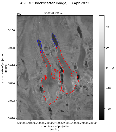
fig, ax = plt.subplots(figsize=(9,8))

power_to_db(vrt_full.vv.mean(dim=['acq_date'])).plot(ax=ax, cmap=plt.cm.Greys_r)

rgi_sub.plot(edgecolor='r', facecolor='none', ax=ax)
rgi_sub.plot(edgecolor='r', facecolor='none', ax=ax)

lakes_prj.plot(ax=ax, facecolor='none', edgecolor='blue')

fig.suptitle('ASF RTC backscatter image, 30 Apr 2022', fontsize=14);

Text(0.5, 0.98, 'ASF RTC backscatter image, 30 Apr 2022')

Clip to lake extent

lake1 = lakes_prj.loc[lakes_prj['id']== 1]
lake2 = lakes_prj.loc[lakes_prj['id'] == 2]

lake1_asf = vrt_full.rio.clip(lake1.geometry, lake1.crs)
lake2_asf = vrt_full.rio.clip(lake2.geometry, lake2.crs)

lake1_asf

<xarray.Dataset>
Dimensions:                           (acq_date: 103, x: 26, y: 51)
Coordinates: (12/17)
  * acq_date                          (acq_date) datetime64[ns] 2021-05-02T12...
  * x                                 (x) float64 6.234e+05 ... 6.242e+05
  * y                                 (y) float64 3.1e+06 3.1e+06 ... 3.098e+06
    sensor                            (acq_date) <U3 'S1A' 'S1A' ... 'S1A' 'S1A'
    beam_mode                         (acq_date) <U2 'IW' 'IW' ... 'IW' 'IW'
    polarisation_type                 (acq_date) <U2 'DV' 'DV' ... 'DV' 'DV'
    ...                                ...
    filtered                          (acq_date) <U1 'n' 'n' 'n' ... 'n' 'n' 'n'
    area                              (acq_date) <U1 'e' 'e' 'e' ... 'e' 'e' 'e'
    product_id                        (acq_date) <U4 '748F' '0D1E' ... 'BD36'
    granule_id                        (acq_date) <U67 'S1A_IW_SLC__1SDV_20210...
    orbital_dir                       (acq_date) <U4 'desc' 'asc' ... 'desc'
    spatial_ref                       int64 0
Data variables:
    vv                                (acq_date, y, x) float32 dask.array<chunksize=(1, 51, 26), meta=np.ndarray>
    vh                                (acq_date, y, x) float32 dask.array<chunksize=(1, 51, 26), meta=np.ndarray>
    ls                                (acq_date, y, x) float64 dask.array<chunksize=(1, 51, 26), meta=np.ndarray>

xarray.Dataset

• Dimensions:
  • acq_date: 103
  • x: 26
  • y: 51
• Coordinates: (17)
  • acq_date
    (acq_date)
    datetime64[ns]
    2021-05-02T12:14:14 ... 2022-05-...

    array(['2021-05-02T12:14:14.000000000', '2021-05-05T00:03:07.000000000',
           '2021-05-09T12:05:42.000000000', '2021-05-14T12:13:49.000000000',
           '2021-05-14T12:14:14.000000000', '2021-05-17T00:03:08.000000000',
           '2021-05-21T12:05:43.000000000', '2021-05-26T12:13:50.000000000',
           '2021-05-29T00:03:09.000000000', '2021-06-02T12:05:43.000000000',
           '2021-06-07T12:13:51.000000000', '2021-06-10T00:03:10.000000000',
           '2021-06-14T12:05:44.000000000', '2021-06-19T12:13:52.000000000',
           '2021-06-22T00:03:10.000000000', '2021-06-26T12:05:45.000000000',
           '2021-07-01T12:13:52.000000000', '2021-07-01T12:14:17.000000000',
           '2021-07-04T00:03:11.000000000', '2021-07-08T12:05:45.000000000',
           '2021-07-13T12:13:53.000000000', '2021-07-13T12:14:18.000000000',
           '2021-07-13T12:14:18.000000000', '2021-07-16T00:03:12.000000000',
           '2021-07-20T12:05:46.000000000', '2021-07-25T12:13:54.000000000',
           '2021-07-28T00:03:12.000000000', '2021-08-01T12:05:47.000000000',
           '2021-08-06T12:13:54.000000000', '2021-08-09T00:03:13.000000000',
           '2021-08-13T12:05:48.000000000', '2021-08-18T12:13:55.000000000',
           '2021-08-21T00:03:14.000000000', '2021-08-25T12:05:48.000000000',
           '2021-08-30T12:13:56.000000000', '2021-09-02T00:03:14.000000000',
           '2021-09-06T12:05:49.000000000', '2021-09-11T12:13:56.000000000',
           '2021-09-14T00:03:15.000000000', '2021-09-18T12:05:49.000000000',
           '2021-09-23T12:13:57.000000000', '2021-09-26T00:03:15.000000000',
           '2021-09-30T12:05:50.000000000', '2021-10-05T12:13:57.000000000',
           '2021-10-08T00:03:15.000000000', '2021-10-12T12:05:50.000000000',
           '2021-10-17T12:13:57.000000000', '2021-10-20T00:03:16.000000000',
           '2021-10-24T12:05:50.000000000', '2021-10-29T12:13:57.000000000',
           '2021-11-01T00:03:15.000000000', '2021-11-05T12:05:49.000000000',
           '2021-11-10T12:13:57.000000000', '2021-11-13T00:03:15.000000000',
           '2021-11-17T12:05:49.000000000', '2021-11-22T12:13:56.000000000',
           '2021-11-25T00:03:15.000000000', '2021-11-29T12:05:49.000000000',
           '2021-12-04T12:13:56.000000000', '2021-12-07T00:03:14.000000000',
           '2021-12-11T12:05:48.000000000', '2021-12-16T12:13:55.000000000',
           '2021-12-19T00:03:14.000000000', '2021-12-23T12:05:48.000000000',
           '2021-12-28T12:13:55.000000000', '2021-12-31T00:03:13.000000000',
           '2022-01-04T12:05:47.000000000', '2022-01-09T12:13:54.000000000',
           '2022-01-12T00:03:13.000000000', '2022-01-16T12:05:47.000000000',
           '2022-01-21T12:13:54.000000000', '2022-01-24T00:03:12.000000000',
           '2022-01-28T12:05:46.000000000', '2022-02-02T12:13:53.000000000',
           '2022-02-05T00:03:12.000000000', '2022-02-09T12:05:46.000000000',
           '2022-02-14T12:13:53.000000000', '2022-02-17T00:03:11.000000000',
           '2022-02-21T12:05:46.000000000', '2022-02-26T12:13:53.000000000',
           '2022-03-01T00:03:11.000000000', '2022-03-05T12:05:45.000000000',
           '2022-03-10T12:13:53.000000000', '2022-03-13T00:03:11.000000000',
           '2022-03-17T12:05:45.000000000', '2022-03-22T12:13:53.000000000',
           '2022-03-25T00:03:12.000000000', '2022-03-29T12:05:46.000000000',
           '2022-04-03T12:13:53.000000000', '2022-04-03T12:14:18.000000000',
           '2022-04-06T00:03:12.000000000', '2022-04-10T12:05:46.000000000',
           '2022-04-15T12:13:53.000000000', '2022-04-18T00:03:12.000000000',
           '2022-04-22T12:05:47.000000000', '2022-04-27T12:13:54.000000000',
           '2022-04-30T00:03:13.000000000', '2022-05-04T12:05:47.000000000',
           '2022-05-09T12:13:55.000000000', '2022-05-16T12:05:48.000000000',
           '2022-05-21T12:13:56.000000000', '2022-05-21T12:14:20.000000000',
           '2022-05-21T12:14:20.000000000'], dtype='datetime64[ns]')

  • x
    (x)
    float64
    6.234e+05 6.234e+05 ... 6.242e+05

    axis :

    X

    long_name :

    x coordinate of projection

    standard_name :

    projection_x_coordinate

    units :

    metre

    array([623415., 623445., 623475., 623505., 623535., 623565., 623595., 623625.,
           623655., 623685., 623715., 623745., 623775., 623805., 623835., 623865.,
           623895., 623925., 623955., 623985., 624015., 624045., 624075., 624105.,
           624135., 624165.])

  • y
    (y)
    float64
    3.1e+06 3.1e+06 ... 3.098e+06

    axis :

    Y

    long_name :

    y coordinate of projection

    standard_name :

    projection_y_coordinate

    units :

    metre

    array([3099675., 3099645., 3099615., 3099585., 3099555., 3099525., 3099495.,
           3099465., 3099435., 3099405., 3099375., 3099345., 3099315., 3099285.,
           3099255., 3099225., 3099195., 3099165., 3099135., 3099105., 3099075.,
           3099045., 3099015., 3098985., 3098955., 3098925., 3098895., 3098865.,
           3098835., 3098805., 3098775., 3098745., 3098715., 3098685., 3098655.,
           3098625., 3098595., 3098565., 3098535., 3098505., 3098475., 3098445.,
           3098415., 3098385., 3098355., 3098325., 3098295., 3098265., 3098235.,
           3098205., 3098175.])

  • sensor
    (acq_date)
    <U3
    'S1A' 'S1A' 'S1A' ... 'S1A' 'S1A'

    array(['S1A', 'S1A', 'S1A', 'S1A', 'S1A', 'S1A', 'S1A', 'S1A', 'S1A',
           'S1A', 'S1A', 'S1A', 'S1A', 'S1A', 'S1A', 'S1A', 'S1A', 'S1A',
           'S1A', 'S1A', 'S1A', 'S1A', 'S1A', 'S1A', 'S1A', 'S1A', 'S1A',
           'S1A', 'S1A', 'S1A', 'S1A', 'S1A', 'S1A', 'S1A', 'S1A', 'S1A',
           'S1A', 'S1A', 'S1A', 'S1A', 'S1A', 'S1A', 'S1A', 'S1A', 'S1A',
           'S1A', 'S1A', 'S1A', 'S1A', 'S1A', 'S1A', 'S1A', 'S1A', 'S1A',
           'S1A', 'S1A', 'S1A', 'S1A', 'S1A', 'S1A', 'S1A', 'S1A', 'S1A',
           'S1A', 'S1A', 'S1A', 'S1A', 'S1A', 'S1A', 'S1A', 'S1A', 'S1A',
           'S1A', 'S1A', 'S1A', 'S1A', 'S1A', 'S1A', 'S1A', 'S1A', 'S1A',
           'S1A', 'S1A', 'S1A', 'S1A', 'S1A', 'S1A', 'S1A', 'S1A', 'S1A',
           'S1A', 'S1A', 'S1A', 'S1A', 'S1A', 'S1A', 'S1A', 'S1A', 'S1A',
           'S1A', 'S1A', 'S1A', 'S1A'], dtype='<U3')

  • beam_mode
    (acq_date)
    <U2
    'IW' 'IW' 'IW' ... 'IW' 'IW' 'IW'

    array(['IW', 'IW', 'IW', 'IW', 'IW', 'IW', 'IW', 'IW', 'IW', 'IW', 'IW',
           'IW', 'IW', 'IW', 'IW', 'IW', 'IW', 'IW', 'IW', 'IW', 'IW', 'IW',
           'IW', 'IW', 'IW', 'IW', 'IW', 'IW', 'IW', 'IW', 'IW', 'IW', 'IW',
           'IW', 'IW', 'IW', 'IW', 'IW', 'IW', 'IW', 'IW', 'IW', 'IW', 'IW',
           'IW', 'IW', 'IW', 'IW', 'IW', 'IW', 'IW', 'IW', 'IW', 'IW', 'IW',
           'IW', 'IW', 'IW', 'IW', 'IW', 'IW', 'IW', 'IW', 'IW', 'IW', 'IW',
           'IW', 'IW', 'IW', 'IW', 'IW', 'IW', 'IW', 'IW', 'IW', 'IW', 'IW',
           'IW', 'IW', 'IW', 'IW', 'IW', 'IW', 'IW', 'IW', 'IW', 'IW', 'IW',
           'IW', 'IW', 'IW', 'IW', 'IW', 'IW', 'IW', 'IW', 'IW', 'IW', 'IW',
           'IW', 'IW', 'IW', 'IW'], dtype='<U2')

  • polarisation_type
    (acq_date)
    <U2
    'DV' 'DV' 'DV' ... 'DV' 'DV' 'DV'

    array(['DV', 'DV', 'DV', 'DV', 'DV', 'DV', 'DV', 'DV', 'DV', 'DV', 'DV',
           'DV', 'DV', 'DV', 'DV', 'DV', 'DV', 'DV', 'DV', 'DV', 'DV', 'DV',
           'DV', 'DV', 'DV', 'DV', 'DV', 'DV', 'DV', 'DV', 'DV', 'DV', 'DV',
           'DV', 'DV', 'DV', 'DV', 'DV', 'DV', 'DV', 'DV', 'DV', 'DV', 'DV',
           'DV', 'DV', 'DV', 'DV', 'DV', 'DV', 'DV', 'DV', 'DV', 'DV', 'DV',
           'DV', 'DV', 'DV', 'DV', 'DV', 'DV', 'DV', 'DV', 'DV', 'DV', 'DV',
           'DV', 'DV', 'DV', 'DV', 'DV', 'DV', 'DV', 'DV', 'DV', 'DV', 'DV',
           'DV', 'DV', 'DV', 'DV', 'DV', 'DV', 'DV', 'DV', 'DV', 'DV', 'DV',
           'DV', 'DV', 'DV', 'DV', 'DV', 'DV', 'DV', 'DV', 'DV', 'DV', 'DV',
           'DV', 'DV', 'DV', 'DV'], dtype='<U2')

  • orbit_type
    (acq_date)
    <U1
    '_' '_' '_' '_' ... '_' '_' '_' '_'

    array(['_', '_', '_', '_', '_', '_', '_', '_', '_', '_', '_', '_', '_',
           '_', '_', '_', '_', '_', '_', '_', '_', '_', '_', '_', '_', '_',
           '_', '_', '_', '_', '_', '_', '_', '_', '_', '_', '_', '_', '_',
           '_', '_', '_', '_', '_', '_', '_', '_', '_', '_', '_', '_', '_',
           '_', '_', '_', '_', '_', '_', '_', '_', '_', '_', '_', '_', '_',
           '_', '_', '_', '_', '_', '_', '_', '_', '_', '_', '_', '_', '_',
           '_', '_', '_', '_', '_', '_', '_', '_', '_', '_', '_', '_', '_',
           '_', '_', '_', '_', '_', '_', '_', '_', '_', '_', '_', '_'],
          dtype='<U1')

  • terrain_correction_pixel_spacing
    (acq_date)
    <U5
    'RTC30' 'RTC30' ... 'RTC30' 'RTC30'

    array(['RTC30', 'RTC30', 'RTC30', 'RTC30', 'RTC30', 'RTC30', 'RTC30',
           'RTC30', 'RTC30', 'RTC30', 'RTC30', 'RTC30', 'RTC30', 'RTC30',
           'RTC30', 'RTC30', 'RTC30', 'RTC30', 'RTC30', 'RTC30', 'RTC30',
           'RTC30', 'RTC30', 'RTC30', 'RTC30', 'RTC30', 'RTC30', 'RTC30',
           'RTC30', 'RTC30', 'RTC30', 'RTC30', 'RTC30', 'RTC30', 'RTC30',
           'RTC30', 'RTC30', 'RTC30', 'RTC30', 'RTC30', 'RTC30', 'RTC30',
           'RTC30', 'RTC30', 'RTC30', 'RTC30', 'RTC30', 'RTC30', 'RTC30',
           'RTC30', 'RTC30', 'RTC30', 'RTC30', 'RTC30', 'RTC30', 'RTC30',
           'RTC30', 'RTC30', 'RTC30', 'RTC30', 'RTC30', 'RTC30', 'RTC30',
           'RTC30', 'RTC30', 'RTC30', 'RTC30', 'RTC30', 'RTC30', 'RTC30',
           'RTC30', 'RTC30', 'RTC30', 'RTC30', 'RTC30', 'RTC30', 'RTC30',
           'RTC30', 'RTC30', 'RTC30', 'RTC30', 'RTC30', 'RTC30', 'RTC30',
           'RTC30', 'RTC30', 'RTC30', 'RTC30', 'RTC30', 'RTC30', 'RTC30',
           'RTC30', 'RTC30', 'RTC30', 'RTC30', 'RTC30', 'RTC30', 'RTC30',
           'RTC30', 'RTC30', 'RTC30', 'RTC30', 'RTC30'], dtype='<U5')

  • output_format
    (acq_date)
    <U1
    'g' 'g' 'g' 'g' ... 'g' 'g' 'g' 'g'

    array(['g', 'g', 'g', 'g', 'g', 'g', 'g', 'g', 'g', 'g', 'g', 'g', 'g',
           'g', 'g', 'g', 'g', 'g', 'g', 'g', 'g', 'g', 'g', 'g', 'g', 'g',
           'g', 'g', 'g', 'g', 'g', 'g', 'g', 'g', 'g', 'g', 'g', 'g', 'g',
           'g', 'g', 'g', 'g', 'g', 'g', 'g', 'g', 'g', 'g', 'g', 'g', 'g',
           'g', 'g', 'g', 'g', 'g', 'g', 'g', 'g', 'g', 'g', 'g', 'g', 'g',
           'g', 'g', 'g', 'g', 'g', 'g', 'g', 'g', 'g', 'g', 'g', 'g', 'g',
           'g', 'g', 'g', 'g', 'g', 'g', 'g', 'g', 'g', 'g', 'g', 'g', 'g',
           'g', 'g', 'g', 'g', 'g', 'g', 'g', 'g', 'g', 'g', 'g', 'g'],
          dtype='<U1')

  • output_type
    (acq_date)
    <U1
    'p' 'p' 'p' 'p' ... 'p' 'p' 'p' 'p'

    array(['p', 'p', 'p', 'p', 'p', 'p', 'p', 'p', 'p', 'p', 'p', 'p', 'p',
           'p', 'p', 'p', 'p', 'p', 'p', 'p', 'p', 'p', 'p', 'p', 'p', 'p',
           'p', 'p', 'p', 'p', 'p', 'p', 'p', 'p', 'p', 'p', 'p', 'p', 'p',
           'p', 'p', 'p', 'p', 'p', 'p', 'p', 'p', 'p', 'p', 'p', 'p', 'p',
           'p', 'p', 'p', 'p', 'p', 'p', 'p', 'p', 'p', 'p', 'p', 'p', 'p',
           'p', 'p', 'p', 'p', 'p', 'p', 'p', 'p', 'p', 'p', 'p', 'p', 'p',
           'p', 'p', 'p', 'p', 'p', 'p', 'p', 'p', 'p', 'p', 'p', 'p', 'p',
           'p', 'p', 'p', 'p', 'p', 'p', 'p', 'p', 'p', 'p', 'p', 'p'],
          dtype='<U1')

  • masked
    (acq_date)
    <U1
    'u' 'u' 'u' 'u' ... 'u' 'u' 'u' 'u'

    array(['u', 'u', 'u', 'u', 'u', 'u', 'u', 'u', 'u', 'u', 'u', 'u', 'u',
           'u', 'u', 'u', 'u', 'u', 'u', 'u', 'u', 'u', 'u', 'u', 'u', 'u',
           'u', 'u', 'u', 'u', 'u', 'u', 'u', 'u', 'u', 'u', 'u', 'u', 'u',
           'u', 'u', 'u', 'u', 'u', 'u', 'u', 'u', 'u', 'u', 'u', 'u', 'u',
           'u', 'u', 'u', 'u', 'u', 'u', 'u', 'u', 'u', 'u', 'u', 'u', 'u',
           'u', 'u', 'u', 'u', 'u', 'u', 'u', 'u', 'u', 'u', 'u', 'u', 'u',
           'u', 'u', 'u', 'u', 'u', 'u', 'u', 'u', 'u', 'u', 'u', 'u', 'u',
           'u', 'u', 'u', 'u', 'u', 'u', 'u', 'u', 'u', 'u', 'u', 'u'],
          dtype='<U1')

  • filtered
    (acq_date)
    <U1
    'n' 'n' 'n' 'n' ... 'n' 'n' 'n' 'n'

    array(['n', 'n', 'n', 'n', 'n', 'n', 'n', 'n', 'n', 'n', 'n', 'n', 'n',
           'n', 'n', 'n', 'n', 'n', 'n', 'n', 'n', 'n', 'n', 'n', 'n', 'n',
           'n', 'n', 'n', 'n', 'n', 'n', 'n', 'n', 'n', 'n', 'n', 'n', 'n',
           'n', 'n', 'n', 'n', 'n', 'n', 'n', 'n', 'n', 'n', 'n', 'n', 'n',
           'n', 'n', 'n', 'n', 'n', 'n', 'n', 'n', 'n', 'n', 'n', 'n', 'n',
           'n', 'n', 'n', 'n', 'n', 'n', 'n', 'n', 'n', 'n', 'n', 'n', 'n',
           'n', 'n', 'n', 'n', 'n', 'n', 'n', 'n', 'n', 'n', 'n', 'n', 'n',
           'n', 'n', 'n', 'n', 'n', 'n', 'n', 'n', 'n', 'n', 'n', 'n'],
          dtype='<U1')

  • area
    (acq_date)
    <U1
    'e' 'e' 'e' 'e' ... 'e' 'e' 'e' 'e'

    array(['e', 'e', 'e', 'e', 'e', 'e', 'e', 'e', 'e', 'e', 'e', 'e', 'e',
           'e', 'e', 'e', 'e', 'e', 'e', 'e', 'e', 'e', 'e', 'e', 'e', 'e',
           'e', 'e', 'e', 'e', 'e', 'e', 'e', 'e', 'e', 'e', 'e', 'e', 'e',
           'e', 'e', 'e', 'e', 'e', 'e', 'e', 'e', 'e', 'e', 'e', 'e', 'e',
           'e', 'e', 'e', 'e', 'e', 'e', 'e', 'e', 'e', 'e', 'e', 'e', 'e',
           'e', 'e', 'e', 'e', 'e', 'e', 'e', 'e', 'e', 'e', 'e', 'e', 'e',
           'e', 'e', 'e', 'e', 'e', 'e', 'e', 'e', 'e', 'e', 'e', 'e', 'e',
           'e', 'e', 'e', 'e', 'e', 'e', 'e', 'e', 'e', 'e', 'e', 'e'],
          dtype='<U1')

  • product_id
    (acq_date)
    <U4
    '748F' '0D1E' ... '01F4' 'BD36'

    array(['748F', '0D1E', '3E89', '61B6', '0535', 'F306', '1380', 'ED8C',
           '2CBE', '1424', 'ABA0', 'E61E', 'E5B6', '5569', '71C9', 'B942',
           'DCE1', 'CA1B', '6581', '1DFD', '5413', '22BD', 'BDC1', '01B2',
           '9849', 'CFFC', '57F2', 'D4E6', 'B7B0', '3770', '52BB', '0579',
           'AA68', '24B8', 'D049', '5FF4', '5F4E', '199D', '0031', 'D082',
           'E74B', 'F7ED', '65E0', 'F587', '528F', '51E7', 'F5AA', 'AC38',
           '772E', 'F0A6', '066E', '5844', '8CD8', '6340', 'D35A', '056C',
           '6E6F', '0CAD', '6270', '8A4F', 'BEAB', '54B1', '8F7B', 'F9A9',
           'AA59', '57E1', '81EB', '250E', '3C39', '3A2A', '9331', 'C14C',
           'F1DE', '106F', 'D48F', '407D', 'FD00', '5D96', '971C', 'F573',
           'C890', '68EA', '83D7', 'E113', 'D846', 'F4B3', 'BB26', '485C',
           'B409', '6683', '6153', '832B', '7418', '378D', '33F5', '1139',
           'B661', '9A2F', '6943', '5BAD', 'FA4F', '01F4', 'BD36'],
          dtype='<U4')

  • granule_id
    (acq_date)
    <U67
    'S1A_IW_SLC__1SDV_20210502T12141...

    array(['S1A_IW_SLC__1SDV_20210502T121414_20210502T121441_037709_047321_900F',
           'S1A_IW_SLC__1SDV_20210505T000307_20210505T000334_037745_047463_4DEF',
           'S1A_IW_SLC__1SDV_20210509T120542_20210509T120609_037811_047676_9EBD',
           'S1A_IW_SLC__1SDV_20210514T121349_20210514T121416_037884_047898_4702',
           'S1A_IW_SLC__1SDV_20210514T121414_20210514T121442_037884_047898_FE6F',
           'S1A_IW_SLC__1SDV_20210517T000308_20210517T000335_037920_0479A9_2A18',
           'S1A_IW_SLC__1SDV_20210521T120543_20210521T120609_037986_047BBD_1CA0',
           'S1A_IW_SLC__1SDV_20210526T121350_20210526T121417_038059_047DE5_0E67',
           'S1A_IW_SLC__1SDV_20210529T000309_20210529T000336_038095_047EF4_5449',
           'S1A_IW_SLC__1SDV_20210602T120543_20210602T120610_038161_0480FD_893F',
           'S1A_IW_SLC__1SDV_20210607T121351_20210607T121418_038234_048318_9B64',
           'S1A_IW_SLC__1SDV_20210610T000310_20210610T000337_038270_04841E_601A',
           'S1A_IW_SLC__1SDV_20210614T120544_20210614T120611_038336_04862F_337B',
           'S1A_IW_SLC__1SDV_20210619T121352_20210619T121419_038409_04884C_1DBA',
           'S1A_IW_SLC__1SDV_20210622T000310_20210622T000337_038445_04895A_842E',
           'S1A_IW_SLC__1SDV_20210626T120545_20210626T120612_038511_048B6C_9585',
           'S1A_IW_SLC__1SDV_20210701T121352_20210701T121419_038584_048D87_F95C',
           'S1A_IW_SLC__1SDV_20210701T121417_20210701T121445_038584_048D87_C79E',
           'S1A_IW_SLC__1SDV_20210704T000311_20210704T000338_038620_048E99_1BAA',
           'S1A_IW_SLC__1SDV_20210708T120545_20210708T120612_038686_0490AD_DD9E',
    ...
           'S1A_IW_SLC__1SDV_20220317T120545_20220317T120612_042361_050CE5_4CCF',
           'S1A_IW_SLC__1SDV_20220322T121353_20220322T121420_042434_050F59_A1B6',
           'S1A_IW_SLC__1SDV_20220325T000312_20220325T000339_042470_051096_BA6F',
           'S1A_IW_SLC__1SDV_20220329T120546_20220329T120613_042536_0512D7_425A',
           'S1A_IW_SLC__1SDV_20220403T121418_20220403T121446_042609_05154A_51E7',
           'S1A_IW_SLC__1SDV_20220403T121353_20220403T121420_042609_05154A_3FE7',
           'S1A_IW_SLC__1SDV_20220406T000312_20220406T000339_042645_051682_4B40',
           'S1A_IW_SLC__1SDV_20220410T120546_20220410T120613_042711_0518C0_3349',
           'S1A_IW_SLC__1SDV_20220415T121353_20220415T121420_042784_051B30_EB87',
           'S1A_IW_SLC__1SDV_20220418T000312_20220418T000339_042820_051C63_CAB2',
           'S1A_IW_SLC__1SDV_20220422T120547_20220422T120614_042886_051E96_41EE',
           'S1A_IW_SLC__1SDV_20220427T121354_20220427T121421_042959_0520EE_A42D',
           'S1A_IW_SLC__1SDV_20220430T000313_20220430T000340_042995_05221E_46A1',
           'S1A_IW_SLC__1SDV_20220504T120547_20220504T120614_043061_05245F_6F62',
           'S1A_IW_SLC__1SDV_20220509T121355_20220509T121422_043134_0526C4_092E',
           'S1A_IW_SLC__1SDV_20220516T120548_20220516T120615_043236_0529DD_42D2',
           'S1A_IW_SLC__1SDV_20220521T121420_20220521T121448_043309_052C00_493D',
           'S1A_IW_SLC__1SDV_20220521T121420_20220521T121448_043309_052C00_493D',
           'S1A_IW_SLC__1SDV_20220521T121356_20220521T121423_043309_052C00_FE88'],
          dtype='<U67')

  • orbital_dir
    (acq_date)
    <U4
    'desc' 'asc' ... 'desc' 'desc'

    array(['desc', 'asc', 'desc', 'desc', 'desc', 'asc', 'desc', 'desc',
           'asc', 'desc', 'desc', 'asc', 'desc', 'desc', 'asc', 'desc',
           'desc', 'desc', 'asc', 'desc', 'desc', 'desc', 'desc', 'asc',
           'desc', 'desc', 'asc', 'desc', 'desc', 'asc', 'desc', 'desc',
           'asc', 'desc', 'desc', 'asc', 'desc', 'desc', 'asc', 'desc',
           'desc', 'asc', 'desc', 'desc', 'asc', 'desc', 'desc', 'asc',
           'desc', 'desc', 'asc', 'desc', 'desc', 'asc', 'desc', 'desc',
           'asc', 'desc', 'desc', 'asc', 'desc', 'desc', 'asc', 'desc',
           'desc', 'asc', 'desc', 'desc', 'asc', 'desc', 'desc', 'asc',
           'desc', 'desc', 'asc', 'desc', 'desc', 'asc', 'desc', 'desc',
           'asc', 'desc', 'desc', 'asc', 'desc', 'desc', 'asc', 'desc',
           'desc', 'desc', 'asc', 'desc', 'desc', 'asc', 'desc', 'desc',
           'asc', 'desc', 'desc', 'desc', 'desc', 'desc', 'desc'], dtype='<U4')

  • spatial_ref
    ()
    int64
    0

    crs_wkt :

    PROJCS["WGS 84 / UTM zone 45N",GEOGCS["WGS 84",DATUM["WGS_1984",SPHEROID["WGS 84",6378137,298.257223563,AUTHORITY["EPSG","7030"]],AUTHORITY["EPSG","6326"]],PRIMEM["Greenwich",0,AUTHORITY["EPSG","8901"]],UNIT["degree",0.0174532925199433,AUTHORITY["EPSG","9122"]],AUTHORITY["EPSG","4326"]],PROJECTION["Transverse_Mercator"],PARAMETER["latitude_of_origin",0],PARAMETER["central_meridian",87],PARAMETER["scale_factor",0.9996],PARAMETER["false_easting",500000],PARAMETER["false_northing",0],UNIT["metre",1,AUTHORITY["EPSG","9001"]],AXIS["Easting",EAST],AXIS["Northing",NORTH],AUTHORITY["EPSG","32645"]]

    semi_major_axis :

    6378137.0

    semi_minor_axis :

    6356752.314245179

    inverse_flattening :

    298.257223563

    reference_ellipsoid_name :

    WGS 84

    longitude_of_prime_meridian :

    0.0

    prime_meridian_name :

    Greenwich

    geographic_crs_name :

    WGS 84

    horizontal_datum_name :

    World Geodetic System 1984

    projected_crs_name :

    WGS 84 / UTM zone 45N

    grid_mapping_name :

    transverse_mercator

    latitude_of_projection_origin :

    0.0

    longitude_of_central_meridian :

    87.0

    false_easting :

    500000.0

    false_northing :

    0.0

    scale_factor_at_central_meridian :

    0.9996

    spatial_ref :

    PROJCS["WGS 84 / UTM zone 45N",GEOGCS["WGS 84",DATUM["WGS_1984",SPHEROID["WGS 84",6378137,298.257223563,AUTHORITY["EPSG","7030"]],AUTHORITY["EPSG","6326"]],PRIMEM["Greenwich",0,AUTHORITY["EPSG","8901"]],UNIT["degree",0.0174532925199433,AUTHORITY["EPSG","9122"]],AUTHORITY["EPSG","4326"]],PROJECTION["Transverse_Mercator"],PARAMETER["latitude_of_origin",0],PARAMETER["central_meridian",87],PARAMETER["scale_factor",0.9996],PARAMETER["false_easting",500000],PARAMETER["false_northing",0],UNIT["metre",1,AUTHORITY["EPSG","9001"]],AXIS["Easting",EAST],AXIS["Northing",NORTH],AUTHORITY["EPSG","32645"]]

    GeoTransform :

    623400.0 30.0 0.0 3099690.0 0.0 -30.0

    array(0)

• Data variables: (3)
  • vv
    (acq_date, y, x)
    float32
    dask.array<chunksize=(1, 51, 26), meta=np.ndarray>

    scale_factor :

    1.0

    add_offset :

    0.0

    _FillValue :

    0.0

    Array Chunk Bytes 533.51 kiB 5.18 kiB Shape (103, 51, 26) (1, 51, 26) Count 20 Graph Layers 103 Chunks Type float32 numpy.ndarray

  • vh
    (acq_date, y, x)
    float32
    dask.array<chunksize=(1, 51, 26), meta=np.ndarray>

    scale_factor :

    1.0

    add_offset :

    0.0

    _FillValue :

    0.0

    Array Chunk Bytes 533.51 kiB 5.18 kiB Shape (103, 51, 26) (1, 51, 26) Count 29 Graph Layers 103 Chunks Type float32 numpy.ndarray

  • ls
    (acq_date, y, x)
    float64
    dask.array<chunksize=(1, 51, 26), meta=np.ndarray>

    scale_factor :

    1.0

    add_offset :

    0.0

    _FillValue :

    0.0

    Array Chunk Bytes 1.04 MiB 10.36 kiB Shape (103, 51, 26) (1, 51, 26) Count 33 Graph Layers 103 Chunks Type float64 numpy.ndarray

• Attributes: (0)

lakes_prj['color'] = ['r','b']
lakes_prj

	id	geometry	color
0	1	POLYGON ((623555.903 3099600.816, 623594.809 3...	r
1	2	POLYGON ((622405.254 3097521.050, 622268.598 3...	b

Data visualization

from matplotlib.lines import Line2D

fig, axs = plt.subplots(ncols = 2, figsize=(18,7))

#scatter plot VV
power_to_db(lake2_asf.vv.mean(dim=['x','y'])).plot(ax=axs[0], color = 'blue', marker='o', linewidth=0, alpha = 0.6);
power_to_db(lake1_asf.vv.mean(dim=['x','y'])).plot(ax=axs[0], color = 'red', marker = 'o', linewidth = 0, alpha = 0.6);

#scatter plot VH
power_to_db(lake2_asf.vh.mean(dim=['x','y'])).plot(ax=axs[1], color = 'blue', marker='o', linewidth=0, alpha = 0.6);
power_to_db(lake1_asf.vh.mean(dim=['x','y'])).plot(ax=axs[1], color = 'red', marker = 'o', linewidth = 0, alpha = 0.6);


axs[0].set_title('VV backscatter over proglacial lakes 2021-2022')
axs[1].set_title('VH backscatter over proglacial lakes 2021-2022')

legend_elements = [Line2D([0], [0], color = 'r', lw = 3, label = 'lake 1'),
                   Line2D([0], [0], color = 'b', lw = 3, label = 'lake 2')]  ;           

/home/emmamarshall/miniconda3/envs/sentinel/lib/python3.10/site-packages/dask/core.py:119: RuntimeWarning: divide by zero encountered in log10
  return func(*(_execute_task(a, cache) for a in args))
/home/emmamarshall/miniconda3/envs/sentinel/lib/python3.10/site-packages/dask/core.py:119: RuntimeWarning: divide by zero encountered in log10
  return func(*(_execute_task(a, cache) for a in args))
/home/emmamarshall/miniconda3/envs/sentinel/lib/python3.10/site-packages/dask/core.py:119: RuntimeWarning: divide by zero encountered in log10
  return func(*(_execute_task(a, cache) for a in args))
/home/emmamarshall/miniconda3/envs/sentinel/lib/python3.10/site-packages/dask/core.py:119: RuntimeWarning: divide by zero encountered in log10
  return func(*(_execute_task(a, cache) for a in args))

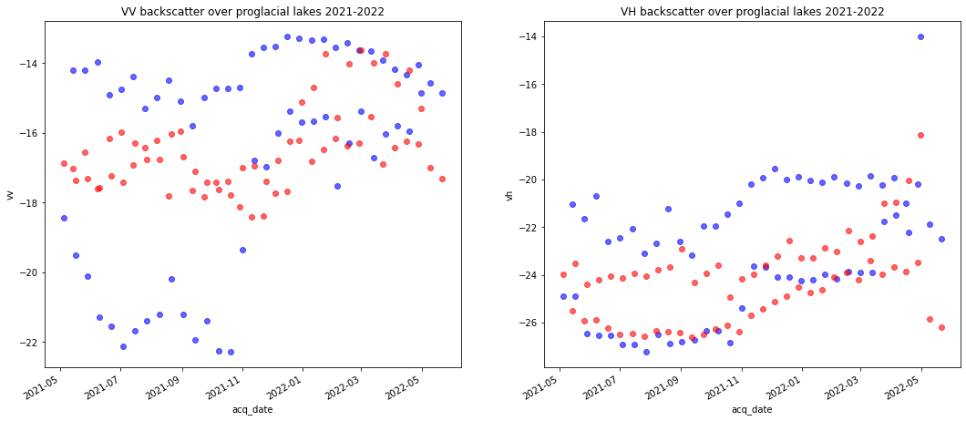
What observations can we make about VV and VH variability in the above plots? What would we want to look at next to further explore those observations?