ASF-processed RTC data inspection

ASF-processed RTC data inspection#

Now that we have read in and organized the stack of Sentinel-1 RTC images, this notebook will demonstrate preliminary dataset inspection.

Learning goals#

Techniques:

Comparing raster images
Using xr.groupby() for grouped statistics
Simple raster calculations
Indexing and selection
Visualizing multiple facets of the data using FacetGrid
Reorganizing data with xr.Dataset.reindex()

Science concepts:

Dataset inspection and evaluation

Other useful resources#

These are resources that contain additional examples and discussion of the content in this notebook and more.

Xarray user guide
How do I… this is very helpful!
Xarray High-level computational patterns discussion of concepts and associated code examples
Parallel computing with dask Xarray tutorial demonstrating wrapping of dask arrays

ASF Data Access#

You can download the RTC-processed backscatter time series here

Software and setup#

%xmode minimal

import os
import xarray as xr
import rioxarray as rio
import geopandas as gpd
from datetime import datetime
import numpy as np
import matplotlib.pyplot as plt
import pandas as pd
import dask

from pathlib import Path

Read in prepared data#

First, we’ll use cell magic to read in the object we prepared in the first notebook:

%store -r vrt_full

vrt_full

<xarray.Dataset>
Dimensions:                           (acq_date: 103, y: 396, x: 290)
Coordinates: (12/17)
  * x                                 (x) float64 6.194e+05 ... 6.281e+05
  * y                                 (y) float64 3.102e+06 ... 3.09e+06
  * acq_date                          (acq_date) datetime64[ns] 2021-05-02T12...
    spatial_ref                       int64 0
    sensor                            (acq_date) <U3 'S1A' 'S1A' ... 'S1A' 'S1A'
    beam_mode                         (acq_date) <U2 'IW' 'IW' ... 'IW' 'IW'
    ...                                ...
    masked                            (acq_date) <U1 'u' 'u' 'u' ... 'u' 'u' 'u'
    filtered                          (acq_date) <U1 'n' 'n' 'n' ... 'n' 'n' 'n'
    area                              (acq_date) <U1 'e' 'e' 'e' ... 'e' 'e' 'e'
    product_id                        (acq_date) <U4 '748F' '0D1E' ... 'BD36'
    granule_id                        (acq_date) <U67 'S1A_IW_SLC__1SDV_20210...
    orbital_dir                       (acq_date) <U4 'desc' 'asc' ... 'desc'
Data variables:
    vv                                (acq_date, y, x) float32 dask.array<chunksize=(1, 396, 290), meta=np.ndarray>
    vh                                (acq_date, y, x) float32 dask.array<chunksize=(1, 396, 290), meta=np.ndarray>
    ls                                (acq_date, y, x) float64 dask.array<chunksize=(1, 396, 290), meta=np.ndarray>

Utility functions#

Lets define two useful functions

To convert from power to dB
To visualize a single time step of ASF and PC data side-by-side

def power_to_db(input_arr):
    return (10*np.log10(np.abs(input_arr)))

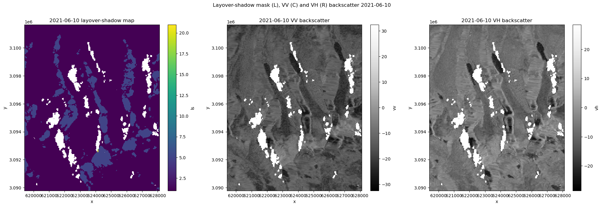
def plot_timestep(input_arr, time_step_int):
    '''plots VV and VH polarizations of a given dataset at a given time step'''
    date = input_arr.isel(acq_date = time_step_int).acq_date.dt.date.data
    fig, axs = plt.subplots(ncols=3, figsize=(24,7))

    input_arr.isel(acq_date=time_step_int).ls.plot(ax=axs[0]);
    power_to_db(input_arr.isel(acq_date=time_step_int).vv).plot(ax=axs[1], cmap = plt.cm.Greys_r);
    power_to_db(input_arr.isel(acq_date=time_step_int).vh).plot(ax=axs[2], cmap = plt.cm.Greys_r);

    fig.suptitle(f'Layover-shadow mask (L), VV (C) and VH (R) backscatter {str(input_arr.isel(acq_date=time_step_int).acq_date.data)[:-19]}')
    axs[0].set_title(f'{date} layover-shadow map')
    axs[1].set_title(f'{date} VV backscatter')
    axs[2].set_title(f'{date} VH backscatter')   

Layover-shadow mask#

Each RTC image comes with a geotiff file containing a layover-shadow mask. This can help to understand missing data you might see in the imagery files. The layover shadow masks are coded to represent a number of different types of pixels:

The following information is copied from the README file that accompanies each scene:

The layover/shadow mask indicates which pixels in the RTC image have been affected by layover and shadow. This layer is tagged with _ls_map.tif

The pixel values are generated by adding the following values together to indicate which layover and shadow effects are impacting each pixel:
 Pixel not tested for layover or shadow
 Pixel tested for layover or shadow
 Pixel has a look angle less than the slope angle
 Pixel is in an area affected by layover
 Pixel has a look angle less than the opposite of the slope angle
Pixel is in an area affected by shadow

There are 17 possible different pixel values, indicating the layover, shadow, and slope conditions present added together for any given pixel._

The values in each cell can range from 0 to 31:
 Not tested for layover or shadow
 Not affected by either layover or shadow
 Look angle < slope angle
 Affected by layover
 Affected by layover; look angle < slope angle
 Look angle < opposite slope angle
Look angle < slope and opposite slope angle
Affected by layover; look angle < opposite slope angle
Affected by layover; look angle < slope and opposite slope angle
Affected by shadow
Affected by shadow; look angle < slope angle
Affected by layover and shadow
Affected by layover and shadow; look angle < slope angle
Affected by shadow; look angle < opposite slope angle
Affected by shadow; look angle < slope and opposite slope angle
Affected by shadow and layover; look angle < opposite slope angle
Affected by shadow and layover; look angle < slope and opposite slope angle

The ASF RTC image product guide has detailed descriptions of how the data is processed and what is included in the processed dataset.

Quick visualization#

plot_timestep(vrt_full, 11)

../_images/1a4ec48607eed8c48a891c7259f9bbf4f782bcca888610bf4670652a979a4d19.png

cmap1 = plt.colormaps['gist_ncar'].resampled(20)

fig, axs = plt.subplots(ncols=2, figsize=(18,9))

vrt_full.isel(acq_date=10).ls.plot(ax=axs[0], vmax=22, vmin=1, cmap=cmap1);
vrt_full.isel(acq_date=11).ls.plot(ax=axs[1], vmax=22, vmin=1, cmap=cmap1);

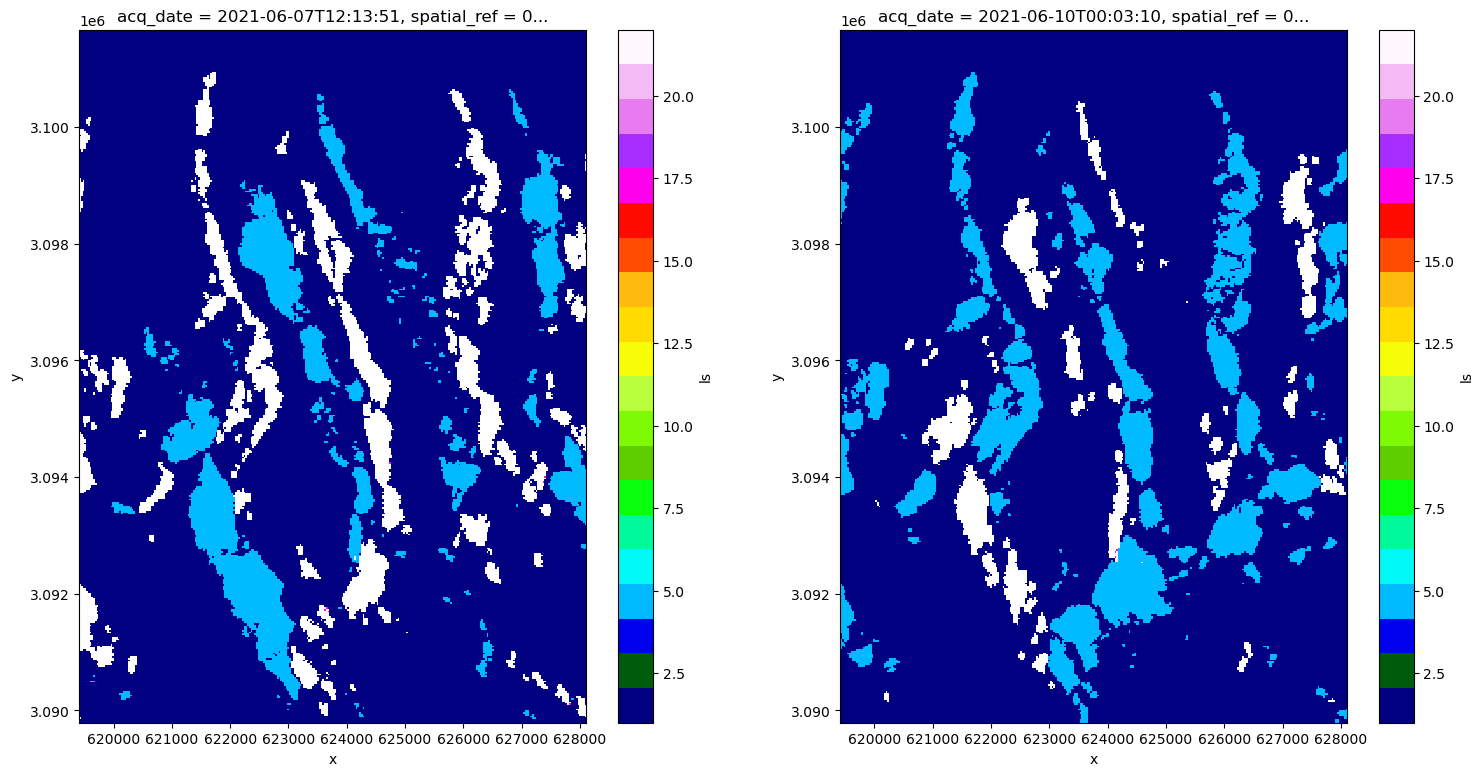
../_images/8a13f3a39990451e152357e50f1a7f2f96cf855de103563696a818d9d2f245a7.png

It looks like there are areas affected by different types of distortion on different dates. For example, in the lower left quadrant, there is a region that is blue (5 - affected by layover) on 6/7/2021 but much of that area appears to be in radar shadow on 6/10/2021. This pattern is present throughout much of the scene with portions of area that are affected by layover in one acquisition in shadow in the next acquisition. This is due to different viewing geometries on different orbital passes: one of the above scenes was likely collected during an ascending pass and one during a descending.

Thanks to all the setup work we did in the previous notebook, we can confirm that:

vrt_full.isel(acq_date=10).orbital_dir.values

array('desc', dtype='<U4')

vrt_full.isel(acq_date=11).orbital_dir.values

array('asc', dtype='<U4')

Looking at backscatter variability#

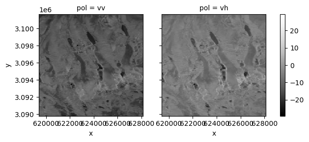
Let’s look at how VV and VH backscatter vary over time.

vrt_vv = vrt_full['vv']
vrt_vh = vrt_full['vh']

mean_pol = xr.Dataset(
    {'vv':vrt_vv.mean('acq_date'), 
     'vh':vrt_vh.mean('acq_date')}
)
power_to_db(mean_pol).to_array('pol').plot(col='pol', cmap=plt.cm.Greys_r);

<xarray.plot.facetgrid.FacetGrid at 0x7fd38ef3c4c0>

../_images/e98fb6fe6f230583138e63b14cdee296fda95b9dd7c83963640a1f0413e23ce4.png

Now let’s look at how backscatter may vary seasonally for a single polarization (for more on time-related GroupBy operations see the Xarray User Guide.

vrt_gb = vrt_full.groupby("acq_date.season").mean()

vrt_gb

<xarray.Dataset>
Dimensions:      (season: 4, y: 396, x: 290)
Coordinates:
  * x            (x) float64 6.194e+05 6.195e+05 ... 6.281e+05 6.281e+05
  * y            (y) float64 3.102e+06 3.102e+06 3.102e+06 ... 3.09e+06 3.09e+06
    spatial_ref  int64 0
  * season       (season) object 'DJF' 'JJA' 'MAM' 'SON'
Data variables:
    vv           (season, y, x) float32 dask.array<chunksize=(1, 396, 290), meta=np.ndarray>
    vh           (season, y, x) float32 dask.array<chunksize=(1, 396, 290), meta=np.ndarray>
    ls           (season, y, x) float64 dask.array<chunksize=(1, 396, 290), meta=np.ndarray>

#order seasons correctly
vrt_gb = vrt_gb.reindex({'season':['DJF','MAM','JJA','SON']})
vrt_gb

<xarray.Dataset>
Dimensions:      (x: 290, y: 396, season: 4)
Coordinates:
  * x            (x) float64 6.194e+05 6.195e+05 ... 6.281e+05 6.281e+05
  * y            (y) float64 3.102e+06 3.102e+06 3.102e+06 ... 3.09e+06 3.09e+06
  * season       (season) <U3 'DJF' 'MAM' 'JJA' 'SON'
    spatial_ref  int64 0
Data variables:
    vv           (season, y, x) float32 dask.array<chunksize=(1, 396, 290), meta=np.ndarray>
    vh           (season, y, x) float32 dask.array<chunksize=(1, 396, 290), meta=np.ndarray>
    ls           (season, y, x) float64 dask.array<chunksize=(1, 396, 290), meta=np.ndarray>

fg_ = power_to_db(vrt_gb.vv).plot(col='season', cmap=plt.cm.Greys_r);

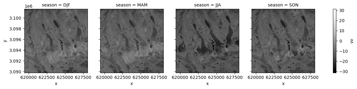
../_images/20b44d8711e025447278c1f06b1a8fe249f79d8400fa547f59a70543f235e24c.png

Interesting, it looks like the winter and spring composites are relatively similar to one another. There also appears to be a decrease in backscatter moving from spring to summer.

Handling duplicate time steps#

If we take a closer look at the ASF dataset, we can see that there are a few scenes from identical acquisitions (can see this in acq_date and more specifically in product_id. Let’s examine these and see what’s going on, if we want to keep the duplicates:

First we’ll extract the data_date_id from the Sentinel-1 granule ID:

data_take_asf = [str(vrt_full.isel(acq_date = t).granule_id.values)[56:62] for t in range(len(vrt_full.acq_date))]

Then assign it as a non-dimensional coordinate:

vrt_full.coords['data_take_id'] = ('acq_date', data_take_asf, {'ID of data take from SAR acquisition':'ID data take'})

asf_ids = list(vrt_full.data_take_id.values)

len(asf_ids)

The length of the asf_ids list is exactly what we’d expect, 103. Let’s look at the number of unique elements using np.unique().

asf_set = np.unique(vrt_full.data_take_id.data)

len(asf_set)

Interesting - it looks like there are only 96 unique elements when we look at the data_take_id. Let’s figure out which are duplicates:

def duplicate(input_ls):
    return list(set([x for x in input_ls if input_ls.count(x) > 1]))

duplicate_ls = duplicate(asf_ids)
duplicate_ls

['048D87', '052C00', '0492D4', '047898', '05154A']

These are the data take IDs that are duplicated in the dataset. We now want to subset the xarray object to only include these data take IDs:

asf_duplicates = vrt_full.where(asf_duplicate_cond==True, drop=True)
asf_duplicates

<xarray.Dataset>
Dimensions:                           (acq_date: 12, y: 396, x: 290)
Coordinates: (12/18)
  * x                                 (x) float64 6.194e+05 ... 6.281e+05
  * y                                 (y) float64 3.102e+06 ... 3.09e+06
  * acq_date                          (acq_date) datetime64[ns] 2021-05-14T12...
    spatial_ref                       int64 0
    sensor                            (acq_date) <U3 'S1A' 'S1A' ... 'S1A' 'S1A'
    beam_mode                         (acq_date) <U2 'IW' 'IW' ... 'IW' 'IW'
    ...                                ...
    filtered                          (acq_date) <U1 'n' 'n' 'n' ... 'n' 'n' 'n'
    area                              (acq_date) <U1 'e' 'e' 'e' ... 'e' 'e' 'e'
    product_id                        (acq_date) <U4 '61B6' '0535' ... 'BD36'
    granule_id                        (acq_date) <U67 'S1A_IW_SLC__1SDV_20210...
    orbital_dir                       (acq_date) <U4 'desc' 'desc' ... 'desc'
    data_take_id                      (acq_date) <U6 '047898' ... '052C00'
Data variables:
    vv                                (acq_date, y, x) float32 dask.array<chunksize=(1, 396, 290), meta=np.ndarray>
    vh                                (acq_date, y, x) float32 dask.array<chunksize=(1, 396, 290), meta=np.ndarray>
    ls                                (acq_date, y, x) float64 dask.array<chunksize=(1, 396, 290), meta=np.ndarray>

Great, now we have a 12-time step xarray object that contains only the duplicate data takes. Let’s see what it looks like. We can use xr.FacetGrid objects to plot these all at once:

fg = asf_duplicates.vv.plot(col='acq_date', col_wrap = 4)

---------------------------------------------------------------------------
ValueError                                Traceback (most recent call last)
Cell In[25], line 1
----> 1 fg = asf_duplicates.vv.plot(col='acq_date', col_wrap = 4)

File ~/miniconda3/envs/s1rtc/lib/python3.10/site-packages/xarray/plot/accessor.py:48, in DataArrayPlotAccessor.__call__(self, **kwargs)
     46 @functools.wraps(dataarray_plot.plot, assigned=("__doc__", "__annotations__"))
     47 def __call__(self, **kwargs) -> Any:
---> 48     return dataarray_plot.plot(self._da, **kwargs)

File ~/miniconda3/envs/s1rtc/lib/python3.10/site-packages/xarray/plot/dataarray_plot.py:309, in plot(darray, row, col, col_wrap, ax, hue, subplot_kws, **kwargs)
    305     plotfunc = hist
    307 kwargs["ax"] = ax
--> 309 return plotfunc(darray, **kwargs)

File ~/miniconda3/envs/s1rtc/lib/python3.10/site-packages/xarray/plot/dataarray_plot.py:1508, in _plot2d.<locals>.newplotfunc(***failed resolving arguments***)
   1506     # Need the decorated plotting function
   1507     allargs["plotfunc"] = globals()[plotfunc.__name__]
-> 1508     return _easy_facetgrid(darray, kind="dataarray", **allargs)
   1510 if darray.ndim == 0 or darray.size == 0:
   1511     # TypeError to be consistent with pandas
   1512     raise TypeError("No numeric data to plot.")

File ~/miniconda3/envs/s1rtc/lib/python3.10/site-packages/xarray/plot/facetgrid.py:1047, in _easy_facetgrid(data, plotfunc, kind, x, y, row, col, col_wrap, sharex, sharey, aspect, size, subplot_kws, ax, figsize, **kwargs)
   1044     sharex = False
   1045     sharey = False
-> 1047 g = FacetGrid(
   1048     data=data,
   1049     col=col,
   1050     row=row,
   1051     col_wrap=col_wrap,
   1052     sharex=sharex,
   1053     sharey=sharey,
   1054     figsize=figsize,
   1055     aspect=aspect,
   1056     size=size,
   1057     subplot_kws=subplot_kws,
   1058 )
   1060 if kind == "line":
   1061     return g.map_dataarray_line(plotfunc, x, y, **kwargs)

File ~/miniconda3/envs/s1rtc/lib/python3.10/site-packages/xarray/plot/facetgrid.py:174, in FacetGrid.__init__(self, data, col, row, col_wrap, sharex, sharey, figsize, aspect, size, subplot_kws)
    172 rep_row = row is not None and not data[row].to_index().is_unique
    173 if rep_col or rep_row:
--> 174     raise ValueError(
    175         "Coordinates used for faceting cannot "
    176         "contain repeated (nonunique) values."
    177     )
    179 # single_group is the grouping variable, if there is exactly one
    180 single_group: bool | Hashable

ValueError: Coordinates used for faceting cannot contain repeated (nonunique) values.

Oops, we can’t use faceting along the acq_date dimension here because of the repeated time steps that we want to look at. Xarray does not know how to handle these repeated values when it is creating the small multiples.

For now we’ll ignore the repeated values to visualize what’s present

fg = asf_duplicates.rename_dims({"acq_date": "step"}).vv.plot(col="step", col_wrap=4)

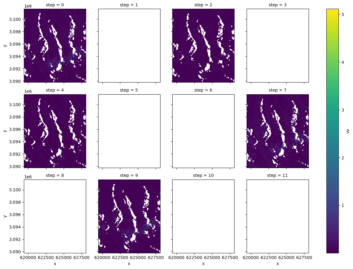
../_images/b492d51a741c337a519b6994db779840e8895698ce934fbe6153905cacb7dc97.png

Interesting, it looks like there’s only really data for the 0, 2, 4, 7 and 9 elements of the list of duplicates.

To drop these, we need to extract the product ID of each duplicate we’d like to remove, since this is the only variable that is unique among the duplicates.

drop_ls = [1,3,5,6,8,10,11]

We can use xarray’s .isel() method, .xr.DataArray.isin(), xr.Dataset.where(), and list comprehension to efficiently subset the time steps we want to keep:

drop_product_id_ls = asf_duplicates.isel(acq_date = drop_ls).product_id.data

drop_product_id_ls

array(['0535', 'CA1B', '22BD', 'BDC1', '6683', '01F4', 'BD36'],
      dtype='<U4')

Using this list, we want to drop all of the elements of vrt_full where product Id is one of the values in the list.

duplicate_cond=~vrt_full.product_id.isin(drop_product_id_ls)

vrt_new = vrt_full.where(duplicate_cond == True, drop=True)

vrt_new

<xarray.Dataset>
Dimensions:                           (acq_date: 96, y: 396, x: 290)
Coordinates: (12/18)
  * x                                 (x) float64 6.194e+05 ... 6.281e+05
  * y                                 (y) float64 3.102e+06 ... 3.09e+06
  * acq_date                          (acq_date) datetime64[ns] 2021-05-02T12...
    spatial_ref                       int64 0
    sensor                            (acq_date) <U3 'S1A' 'S1A' ... 'S1A' 'S1A'
    beam_mode                         (acq_date) <U2 'IW' 'IW' ... 'IW' 'IW'
    ...                                ...
    filtered                          (acq_date) <U1 'n' 'n' 'n' ... 'n' 'n' 'n'
    area                              (acq_date) <U1 'e' 'e' 'e' ... 'e' 'e' 'e'
    product_id                        (acq_date) <U4 '748F' '0D1E' ... 'FA4F'
    granule_id                        (acq_date) <U67 'S1A_IW_SLC__1SDV_20210...
    orbital_dir                       (acq_date) <U4 'desc' 'asc' ... 'desc'
    data_take_id                      (acq_date) <U6 '047321' ... '052C00'
Data variables:
    vv                                (acq_date, y, x) float32 dask.array<chunksize=(1, 396, 290), meta=np.ndarray>
    vh                                (acq_date, y, x) float32 dask.array<chunksize=(1, 396, 290), meta=np.ndarray>
    ls                                (acq_date, y, x) float64 dask.array<chunksize=(1, 396, 290), meta=np.ndarray>

#vrt_new = vrt_full.sel(~vrt_full.product_id.isin(drop_product_id_ls)==True)

vrt_new

<xarray.Dataset>
Dimensions:                           (acq_date: 96, y: 396, x: 290)
Coordinates: (12/18)
  * x                                 (x) float64 6.194e+05 ... 6.281e+05
  * y                                 (y) float64 3.102e+06 ... 3.09e+06
  * acq_date                          (acq_date) datetime64[ns] 2021-05-02T12...
    spatial_ref                       int64 0
    sensor                            (acq_date) <U3 'S1A' 'S1A' ... 'S1A' 'S1A'
    beam_mode                         (acq_date) <U2 'IW' 'IW' ... 'IW' 'IW'
    ...                                ...
    filtered                          (acq_date) <U1 'n' 'n' 'n' ... 'n' 'n' 'n'
    area                              (acq_date) <U1 'e' 'e' 'e' ... 'e' 'e' 'e'
    product_id                        (acq_date) <U4 '748F' '0D1E' ... 'FA4F'
    granule_id                        (acq_date) <U67 'S1A_IW_SLC__1SDV_20210...
    orbital_dir                       (acq_date) <U4 'desc' 'asc' ... 'desc'
    data_take_id                      (acq_date) <U6 '047321' ... '052C00'
Data variables:
    vv                                (acq_date, y, x) float32 dask.array<chunksize=(1, 396, 290), meta=np.ndarray>
    vh                                (acq_date, y, x) float32 dask.array<chunksize=(1, 396, 290), meta=np.ndarray>
    ls                                (acq_date, y, x) float64 dask.array<chunksize=(1, 396, 290), meta=np.ndarray>

Now we will store the updated version of vrt_full (vrt_new) to use in later notebooks:

%store vrt_new

Stored 'vrt_new' (Dataset)

Wrap up#

This notebook gives a brief look in to the vast amount of auxiliary data that is contained within this dataset. Making the most and best use of this dataset requires familiarity with the the many different types of information it includes.