4. Exploratory data analysis of multiple glaciers
Introduction
The previous notebooks in this tutorial demonstrated how to use Xarray to access, inspect, manipulate and analyze raster time series data at the scale of an individual glacier. In this notebook, we shift our focus to a sub-regional scale, looking at all of the glaciers within a given ITS_LIVE data cube. This workflow will draw on elements from the past notebooks while introducing new tools for examining raster data along temporal and spatial dimensions (ie. across multiple glaciers).
Outline
Raster data
Vector data
**B. Combine raster and vector data to create a vector data cube
Make a vector data cube
Add attribute data to vector cube
Write vector cube to disk
Read vector data cube into memory
Visualize velocity data
Visualize associations between velocity and attribute data
Learning goals
Concepts
Querying and accessing raster data from cloud object storage
Accessing and manipulating vector data
Handling coordinate reference information
Calculating and visualizing summary statistics
Techniques
Reading GeoParquet vector data using GeoPandas
Rasterize vector objects using Geocube
Spatial joins of vector datasets using GeoPandas
Using dask to work with out-of-memory data
Data visualization using Pandas
Interactive data visualization with GeoPandas
Expand the next cell to see specific packages used in this notebook and relevant system and version information.
Show code cell source Hide code cell source
%xmode minimal

import contextily as cx
import dask
from dask.diagnostics import ProgressBar
import geopandas as gpd
import matplotlib.pyplot as plt
import numpy as np
import pandas as pd
import rioxarray as rxr
import xarray as xr
import xvec

import itslivetools

%config InlineBackend.figure_format='retina'
Exception reporting mode: Minimal
A. Read and organize data#
1) Raster data#
As in past notebooks, we use itslivetools.find_granule_by_point() to query the ITS_LIVE catalog for the correct url.
itslive_catalog = gpd.read_file('https://its-live-data.s3.amazonaws.com/datacubes/catalog_v02.json')
url = itslivetools.find_granule_by_point([95.180191, 30.645973])
url
'http://its-live-data.s3.amazonaws.com/datacubes/v2-updated-october2024/N30E090/ITS_LIVE_vel_EPSG32646_G0120_X750000_Y3350000.zarr'
Following the example shown in the initial data inspection notebook, we read the data in without dask at first so that we can lazily organize the dataset in chronological order
dc = itslivetools.read_in_s3(url, chunks_arg=None)
dc = dc.sortby('mid_date')
dc
<xarray.Dataset> Size: 1TB
Dimensions:                     (mid_date: 47892, y: 833, x: 833)
Coordinates:
  * mid_date                    (mid_date) datetime64[ns] 383kB 1986-09-11T03...
  * x                           (x) float64 7kB 7.001e+05 7.003e+05 ... 8e+05
  * y                           (y) float64 7kB 3.4e+06 3.4e+06 ... 3.3e+06
Data variables: (12/60)
    M11                         (mid_date, y, x) float32 133GB ...
    M11_dr_to_vr_factor         (mid_date) float32 192kB ...
    M12                         (mid_date, y, x) float32 133GB ...
    M12_dr_to_vr_factor         (mid_date) float32 192kB ...
    acquisition_date_img1       (mid_date) datetime64[ns] 383kB ...
    acquisition_date_img2       (mid_date) datetime64[ns] 383kB ...
    ...                          ...
    vy_error_modeled            (mid_date) float32 192kB ...
    vy_error_slow               (mid_date) float32 192kB ...
    vy_error_stationary         (mid_date) float32 192kB ...
    vy_stable_shift             (mid_date) float32 192kB ...
    vy_stable_shift_slow        (mid_date) float32 192kB ...
    vy_stable_shift_stationary  (mid_date) float32 192kB ...
Attributes: (12/19)
    Conventions:                CF-1.8
    GDAL_AREA_OR_POINT:         Area
    author:                     ITS_LIVE, a NASA MEaSUREs project (its-live.j...
    autoRIFT_parameter_file:    http://its-live-data.s3.amazonaws.com/autorif...
    datacube_software_version:  1.0
    date_created:               25-Sep-2023 22:00:23
    ...                         ...
    s3:                         s3://its-live-data/datacubes/v2/N30E090/ITS_L...
    skipped_granules:           s3://its-live-data/datacubes/v2/N30E090/ITS_L...
    time_standard_img1:         UTC
    time_standard_img2:         UTC
    title:                      ITS_LIVE datacube of image pair velocities
url: https://its-live-data.s3.amazonaws.com/datacu...- mid_date: 47892
- y: 833
- x: 833
- mid_date(mid_date)datetime64[ns]1986-09-11T03:31:15.003252992 .....
- description :
- midpoint of image 1 and image 2 acquisition date and time with granule's centroid longitude and latitude as microseconds
- standard_name :
- image_pair_center_date_with_time_separation
array(['1986-09-11T03:31:15.003252992', '1986-10-05T03:31:06.144750016', '1986-10-21T03:31:34.493249984', ..., '2024-10-29T04:18:09.241024000', '2024-10-29T04:18:09.241024000', '2024-10-29T04:18:09.241024000'], dtype='datetime64[ns]') - x(x)float647.001e+05 7.003e+05 ... 8e+05
- description :
- x coordinate of projection
- standard_name :
- projection_x_coordinate
array([700132.5, 700252.5, 700372.5, ..., 799732.5, 799852.5, 799972.5])
- y(y)float643.4e+06 3.4e+06 ... 3.3e+06 3.3e+06
- description :
- y coordinate of projection
- standard_name :
- projection_y_coordinate
array([3399907.5, 3399787.5, 3399667.5, ..., 3300307.5, 3300187.5, 3300067.5])
- M11(mid_date, y, x)float32...
- description :
- conversion matrix element (1st row, 1st column) that can be multiplied with vx to give range pixel displacement dr (see Eq. A18 in https://www.mdpi.com/2072-4292/13/4/749)
- grid_mapping :
- mapping
- standard_name :
- conversion_matrix_element_11
- units :
- pixel/(meter/year)
[33231731988 values with dtype=float32]
- M11_dr_to_vr_factor(mid_date)float32...
- description :
- multiplicative factor that converts slant range pixel displacement dr to slant range velocity vr
- standard_name :
- M11_dr_to_vr_factor
- units :
- meter/(year*pixel)
[47892 values with dtype=float32]
- M12(mid_date, y, x)float32...
- description :
- conversion matrix element (1st row, 2nd column) that can be multiplied with vy to give range pixel displacement dr (see Eq. A18 in https://www.mdpi.com/2072-4292/13/4/749)
- grid_mapping :
- mapping
- standard_name :
- conversion_matrix_element_12
- units :
- pixel/(meter/year)
[33231731988 values with dtype=float32]
- M12_dr_to_vr_factor(mid_date)float32...
- description :
- multiplicative factor that converts slant range pixel displacement dr to slant range velocity vr
- standard_name :
- M12_dr_to_vr_factor
- units :
- meter/(year*pixel)
[47892 values with dtype=float32]
- acquisition_date_img1(mid_date)datetime64[ns]...
- description :
- acquisition date and time of image 1
- standard_name :
- image1_acquition_date
[47892 values with dtype=datetime64[ns]]
- acquisition_date_img2(mid_date)datetime64[ns]...
- description :
- acquisition date and time of image 2
- standard_name :
- image2_acquition_date
[47892 values with dtype=datetime64[ns]]
- autoRIFT_software_version(mid_date)<U5...
- description :
- version of autoRIFT software
- standard_name :
- autoRIFT_software_version
[47892 values with dtype=<U5]
- chip_size_height(mid_date, y, x)float32...
- chip_size_coordinates :
- Optical data: chip_size_coordinates = 'image projection geometry: width = x, height = y'. Radar data: chip_size_coordinates = 'radar geometry: width = range, height = azimuth'
- description :
- height of search template (chip)
- grid_mapping :
- mapping
- standard_name :
- chip_size_height
- units :
- m
- y_pixel_size :
- 10.0
[33231731988 values with dtype=float32]
- chip_size_width(mid_date, y, x)float32...
- chip_size_coordinates :
- Optical data: chip_size_coordinates = 'image projection geometry: width = x, height = y'. Radar data: chip_size_coordinates = 'radar geometry: width = range, height = azimuth'
- description :
- width of search template (chip)
- grid_mapping :
- mapping
- standard_name :
- chip_size_width
- units :
- m
- x_pixel_size :
- 10.0
[33231731988 values with dtype=float32]
- date_center(mid_date)datetime64[ns]...
- description :
- midpoint of image 1 and image 2 acquisition date
- standard_name :
- image_pair_center_date
[47892 values with dtype=datetime64[ns]]
- date_dt(mid_date)timedelta64[ns]...
- description :
- time separation between acquisition of image 1 and image 2
- standard_name :
- image_pair_time_separation
[47892 values with dtype=timedelta64[ns]]
- floatingice(y, x)float32...
- description :
- floating ice mask, 0 = non-floating-ice, 1 = floating-ice
- flag_meanings :
- non-ice ice
- flag_values :
- [0, 1]
- grid_mapping :
- mapping
- standard_name :
- floating ice mask
- url :
- https://its-live-data.s3.amazonaws.com/autorift_parameters/v001/N46_0120m_floatingice.tif
[693889 values with dtype=float32]
- granule_url(mid_date)<U1024...
- description :
- original granule URL
- standard_name :
- granule_url
[47892 values with dtype=<U1024]
- interp_mask(mid_date, y, x)float32...
- description :
- light interpolation mask
- flag_meanings :
- measured interpolated
- flag_values :
- [0, 1]
- grid_mapping :
- mapping
- standard_name :
- interpolated_value_mask
[33231731988 values with dtype=float32]
- landice(y, x)float32...
- description :
- land ice mask, 0 = non-land-ice, 1 = land-ice
- flag_meanings :
- non-ice ice
- flag_values :
- [0, 1]
- grid_mapping :
- mapping
- standard_name :
- land ice mask
- url :
- https://its-live-data.s3.amazonaws.com/autorift_parameters/v001/N46_0120m_landice.tif
[693889 values with dtype=float32]
- mapping()<U1...
- GeoTransform :
- 700072.5 120.0 0 3399967.5 0 -120.0
- crs_wkt :
- PROJCS["WGS 84 / UTM zone 46N",GEOGCS["WGS 84",DATUM["WGS_1984",SPHEROID["WGS 84",6378137,298.257223563,AUTHORITY["EPSG","7030"]],AUTHORITY["EPSG","6326"]],PRIMEM["Greenwich",0,AUTHORITY["EPSG","8901"]],UNIT["degree",0.0174532925199433,AUTHORITY["EPSG","9122"]],AUTHORITY["EPSG","4326"]],PROJECTION["Transverse_Mercator"],PARAMETER["latitude_of_origin",0],PARAMETER["central_meridian",93],PARAMETER["scale_factor",0.9996],PARAMETER["false_easting",500000],PARAMETER["false_northing",0],UNIT["metre",1,AUTHORITY["EPSG","9001"]],AXIS["Easting",EAST],AXIS["Northing",NORTH],AUTHORITY["EPSG","32646"]]
- false_easting :
- 500000.0
- false_northing :
- 0.0
- grid_mapping_name :
- universal_transverse_mercator
- inverse_flattening :
- 298.257223563
- latitude_of_projection_origin :
- 0.0
- longitude_of_central_meridian :
- 93.0
- proj4text :
- +proj=utm +zone=46 +datum=WGS84 +units=m +no_defs
- scale_factor_at_central_meridian :
- 0.9996
- semi_major_axis :
- 6378137.0
- spatial_epsg :
- 32646
- spatial_ref :
- PROJCS["WGS 84 / UTM zone 46N",GEOGCS["WGS 84",DATUM["WGS_1984",SPHEROID["WGS 84",6378137,298.257223563,AUTHORITY["EPSG","7030"]],AUTHORITY["EPSG","6326"]],PRIMEM["Greenwich",0,AUTHORITY["EPSG","8901"]],UNIT["degree",0.0174532925199433,AUTHORITY["EPSG","9122"]],AUTHORITY["EPSG","4326"]],PROJECTION["Transverse_Mercator"],PARAMETER["latitude_of_origin",0],PARAMETER["central_meridian",93],PARAMETER["scale_factor",0.9996],PARAMETER["false_easting",500000],PARAMETER["false_northing",0],UNIT["metre",1,AUTHORITY["EPSG","9001"]],AXIS["Easting",EAST],AXIS["Northing",NORTH],AUTHORITY["EPSG","32646"]]
- utm_zone_number :
- 46.0
[1 values with dtype=<U1]
- mission_img1(mid_date)<U1...
- description :
- id of the mission that acquired image 1
- standard_name :
- image1_mission
[47892 values with dtype=<U1]
- mission_img2(mid_date)<U1...
- description :
- id of the mission that acquired image 2
- standard_name :
- image2_mission
[47892 values with dtype=<U1]
- roi_valid_percentage(mid_date)float32...
- description :
- percentage of pixels with a valid velocity estimate determined for the intersection of the full image pair footprint and the region of interest (roi) that defines where autoRIFT tried to estimate a velocity
- standard_name :
- region_of_interest_valid_pixel_percentage
[47892 values with dtype=float32]
- satellite_img1(mid_date)<U2...
- description :
- id of the satellite that acquired image 1
- standard_name :
- image1_satellite
[47892 values with dtype=<U2]
- satellite_img2(mid_date)<U2...
- description :
- id of the satellite that acquired image 2
- standard_name :
- image2_satellite
[47892 values with dtype=<U2]
- sensor_img1(mid_date)<U3...
- description :
- id of the sensor that acquired image 1
- standard_name :
- image1_sensor
[47892 values with dtype=<U3]
- sensor_img2(mid_date)<U3...
- description :
- id of the sensor that acquired image 2
- standard_name :
- image2_sensor
[47892 values with dtype=<U3]
- stable_count_slow(mid_date)uint16...
- description :
- number of valid pixels over slowest 25% of ice
- standard_name :
- stable_count_slow
- units :
- count
[47892 values with dtype=uint16]
- stable_count_stationary(mid_date)uint16...
- description :
- number of valid pixels over stationary or slow-flowing surfaces
- standard_name :
- stable_count_stationary
- units :
- count
[47892 values with dtype=uint16]
- stable_shift_flag(mid_date)uint8...
- description :
- flag for applying velocity bias correction: 0 = no correction; 1 = correction from overlapping stable surface mask (stationary or slow-flowing surfaces with velocity < 15 m/yr)(top priority); 2 = correction from slowest 25% of overlapping velocities (second priority)
- standard_name :
- stable_shift_flag
[47892 values with dtype=uint8]
- v(mid_date, y, x)float32...
- description :
- velocity magnitude
- grid_mapping :
- mapping
- standard_name :
- land_ice_surface_velocity
- units :
- meter/year
[33231731988 values with dtype=float32]
- v_error(mid_date, y, x)float32...
- description :
- velocity magnitude error
- grid_mapping :
- mapping
- standard_name :
- velocity_error
- units :
- meter/year
[33231731988 values with dtype=float32]
- va(mid_date, y, x)float32...
- description :
- velocity in radar azimuth direction
- grid_mapping :
- mapping
[33231731988 values with dtype=float32]
- va_error(mid_date)float32...
- description :
- error for velocity in radar azimuth direction
- standard_name :
- va_error
- units :
- meter/year
[47892 values with dtype=float32]
- va_error_modeled(mid_date)float32...
- description :
- 1-sigma error calculated using a modeled error-dt relationship
- standard_name :
- va_error_modeled
- units :
- meter/year
[47892 values with dtype=float32]
- va_error_slow(mid_date)float32...
- description :
- RMSE over slowest 25% of retrieved velocities
- standard_name :
- va_error_slow
- units :
- meter/year
[47892 values with dtype=float32]
- va_error_stationary(mid_date)float32...
- description :
- RMSE over stable surfaces, stationary or slow-flowing surfaces with velocity < 15 m/yr identified from an external mask
- standard_name :
- va_error_stationary
- units :
- meter/year
[47892 values with dtype=float32]
- va_stable_shift(mid_date)float32...
- description :
- applied va shift calibrated using pixels over stable or slow surfaces
- standard_name :
- va_stable_shift
- units :
- meter/year
[47892 values with dtype=float32]
- va_stable_shift_slow(mid_date)float32...
- description :
- va shift calibrated using valid pixels over slowest 25% of retrieved velocities
- standard_name :
- va_stable_shift_slow
- units :
- meter/year
[47892 values with dtype=float32]
- va_stable_shift_stationary(mid_date)float32...
- description :
- va shift calibrated using valid pixels over stable surfaces, stationary or slow-flowing surfaces with velocity < 15 m/yr identified from an external mask
- standard_name :
- va_stable_shift_stationary
- units :
- meter/year
[47892 values with dtype=float32]
- vr(mid_date, y, x)float32...
- description :
- velocity in radar range direction
- grid_mapping :
- mapping
[33231731988 values with dtype=float32]
- vr_error(mid_date)float32...
- description :
- error for velocity in radar range direction
- standard_name :
- vr_error
- units :
- meter/year
[47892 values with dtype=float32]
- vr_error_modeled(mid_date)float32...
- description :
- 1-sigma error calculated using a modeled error-dt relationship
- standard_name :
- vr_error_modeled
- units :
- meter/year
[47892 values with dtype=float32]
- vr_error_slow(mid_date)float32...
- description :
- RMSE over slowest 25% of retrieved velocities
- standard_name :
- vr_error_slow
- units :
- meter/year
[47892 values with dtype=float32]
- vr_error_stationary(mid_date)float32...
- description :
- RMSE over stable surfaces, stationary or slow-flowing surfaces with velocity < 15 m/yr identified from an external mask
- standard_name :
- vr_error_stationary
- units :
- meter/year
[47892 values with dtype=float32]
- vr_stable_shift(mid_date)float32...
- description :
- applied vr shift calibrated using pixels over stable or slow surfaces
- standard_name :
- vr_stable_shift
- units :
- meter/year
[47892 values with dtype=float32]
- vr_stable_shift_slow(mid_date)float32...
- description :
- vr shift calibrated using valid pixels over slowest 25% of retrieved velocities
- standard_name :
- vr_stable_shift_slow
- units :
- meter/year
[47892 values with dtype=float32]
- vr_stable_shift_stationary(mid_date)float32...
- description :
- vr shift calibrated using valid pixels over stable surfaces, stationary or slow-flowing surfaces with velocity < 15 m/yr identified from an external mask
- standard_name :
- vr_stable_shift_stationary
- units :
- meter/year
[47892 values with dtype=float32]
- vx(mid_date, y, x)float32...
- description :
- velocity component in x direction
- grid_mapping :
- mapping
- standard_name :
- land_ice_surface_x_velocity
- units :
- meter/year
[33231731988 values with dtype=float32]
- vx_error(mid_date)float32...
- description :
- best estimate of x_velocity error: vx_error is populated according to the approach used for the velocity bias correction as indicated in "stable_shift_flag"
- standard_name :
- vx_error
- units :
- meter/year
[47892 values with dtype=float32]
- vx_error_modeled(mid_date)float32...
- description :
- 1-sigma error calculated using a modeled error-dt relationship
- standard_name :
- vx_error_modeled
- units :
- meter/year
[47892 values with dtype=float32]
- vx_error_slow(mid_date)float32...
- description :
- RMSE over slowest 25% of retrieved velocities
- standard_name :
- vx_error_slow
- units :
- meter/year
[47892 values with dtype=float32]
- vx_error_stationary(mid_date)float32...
- description :
- RMSE over stable surfaces, stationary or slow-flowing surfaces with velocity < 15 meter/year identified from an external mask
- standard_name :
- vx_error_stationary
- units :
- meter/year
[47892 values with dtype=float32]
- vx_stable_shift(mid_date)float32...
- description :
- applied vx shift calibrated using pixels over stable or slow surfaces
- standard_name :
- vx_stable_shift
- units :
- meter/year
[47892 values with dtype=float32]
- vx_stable_shift_slow(mid_date)float32...
- description :
- vx shift calibrated using valid pixels over slowest 25% of retrieved velocities
- standard_name :
- vx_stable_shift_slow
- units :
- meter/year
[47892 values with dtype=float32]
- vx_stable_shift_stationary(mid_date)float32...
- description :
- vx shift calibrated using valid pixels over stable surfaces, stationary or slow-flowing surfaces with velocity < 15 m/yr identified from an external mask
- standard_name :
- vx_stable_shift_stationary
- units :
- meter/year
[47892 values with dtype=float32]
- vy(mid_date, y, x)float32...
- description :
- velocity component in y direction
- grid_mapping :
- mapping
- standard_name :
- land_ice_surface_y_velocity
- units :
- meter/year
[33231731988 values with dtype=float32]
- vy_error(mid_date)float32...
- description :
- best estimate of y_velocity error: vy_error is populated according to the approach used for the velocity bias correction as indicated in "stable_shift_flag"
- standard_name :
- vy_error
- units :
- meter/year
[47892 values with dtype=float32]
- vy_error_modeled(mid_date)float32...
- description :
- 1-sigma error calculated using a modeled error-dt relationship
- standard_name :
- vy_error_modeled
- units :
- meter/year
[47892 values with dtype=float32]
- vy_error_slow(mid_date)float32...
- description :
- RMSE over slowest 25% of retrieved velocities
- standard_name :
- vy_error_slow
- units :
- meter/year
[47892 values with dtype=float32]
- vy_error_stationary(mid_date)float32...
- description :
- RMSE over stable surfaces, stationary or slow-flowing surfaces with velocity < 15 meter/year identified from an external mask
- standard_name :
- vy_error_stationary
- units :
- meter/year
[47892 values with dtype=float32]
- vy_stable_shift(mid_date)float32...
- description :
- applied vy shift calibrated using pixels over stable or slow surfaces
- standard_name :
- vy_stable_shift
- units :
- meter/year
[47892 values with dtype=float32]
- vy_stable_shift_slow(mid_date)float32...
- description :
- vy shift calibrated using valid pixels over slowest 25% of retrieved velocities
- standard_name :
- vy_stable_shift_slow
- units :
- meter/year
[47892 values with dtype=float32]
- vy_stable_shift_stationary(mid_date)float32...
- description :
- vy shift calibrated using valid pixels over stable surfaces, stationary or slow-flowing surfaces with velocity < 15 m/yr identified from an external mask
- standard_name :
- vy_stable_shift_stationary
- units :
- meter/year
[47892 values with dtype=float32]
- mid_datePandasIndex
PandasIndex(DatetimeIndex(['1986-09-11 03:31:15.003252992', '1986-10-05 03:31:06.144750016', '1986-10-21 03:31:34.493249984', '1986-11-22 03:29:27.023556992', '1986-11-30 03:29:08.710132992', '1986-12-08 03:29:55.372057024', '1986-12-08 03:33:17.095283968', '1986-12-16 03:30:10.645544', '1986-12-24 03:29:52.332120960', '1987-01-09 03:30:01.787228992', ... '2024-10-21 16:17:50.241008896', '2024-10-24 04:17:34.241014016', '2024-10-24 04:17:34.241014016', '2024-10-24 04:17:34.241014016', '2024-10-24 04:17:34.241014016', '2024-10-25 04:10:35.189837056', '2024-10-29 04:18:09.241024', '2024-10-29 04:18:09.241024', '2024-10-29 04:18:09.241024', '2024-10-29 04:18:09.241024'], dtype='datetime64[ns]', name='mid_date', length=47892, freq=None)) - xPandasIndex
PandasIndex(Index([700132.5, 700252.5, 700372.5, 700492.5, 700612.5, 700732.5, 700852.5, 700972.5, 701092.5, 701212.5, ... 798892.5, 799012.5, 799132.5, 799252.5, 799372.5, 799492.5, 799612.5, 799732.5, 799852.5, 799972.5], dtype='float64', name='x', length=833)) - yPandasIndex
PandasIndex(Index([3399907.5, 3399787.5, 3399667.5, 3399547.5, 3399427.5, 3399307.5,
       3399187.5, 3399067.5, 3398947.5, 3398827.5,
       ...
       3301147.5, 3301027.5, 3300907.5, 3300787.5, 3300667.5, 3300547.5,
       3300427.5, 3300307.5, 3300187.5, 3300067.5],
      dtype='float64', name='y', length=833))
- Conventions :
- CF-1.8
- GDAL_AREA_OR_POINT :
- Area
- author :
- ITS_LIVE, a NASA MEaSUREs project (its-live.jpl.nasa.gov)
- autoRIFT_parameter_file :
- http://its-live-data.s3.amazonaws.com/autorift_parameters/v001/autorift_landice_0120m.shp
- datacube_software_version :
- 1.0
- date_created :
- 25-Sep-2023 22:00:23
- date_updated :
- 13-Nov-2024 00:08:07
- geo_polygon :
- [[95.06959008486952, 29.814255053135895], [95.32812062059084, 29.809951334550703], [95.58659184122865, 29.80514261876954], [95.84499718862224, 29.7998293459177], [96.10333011481168, 29.79401200205343], [96.11032804508507, 30.019297601073085], [96.11740568350054, 30.244573983323825], [96.12456379063154, 30.469841094022847], [96.1318031397002, 30.695098878594504], [95.87110827645229, 30.70112924501256], [95.61033817656023, 30.7066371044805], [95.34949964126946, 30.711621947056347], [95.08859948278467, 30.716083310981194], [95.08376623410525, 30.49063893600811], [95.07898726183609, 30.26518607254204], [95.0742620484426, 30.039724763743482], [95.06959008486952, 29.814255053135895]]
- institution :
- NASA Jet Propulsion Laboratory (JPL), California Institute of Technology
- latitude :
- 30.26
- longitude :
- 95.6
- proj_polygon :
- [[700000, 3300000], [725000.0, 3300000.0], [750000.0, 3300000.0], [775000.0, 3300000.0], [800000, 3300000], [800000.0, 3325000.0], [800000.0, 3350000.0], [800000.0, 3375000.0], [800000, 3400000], [775000.0, 3400000.0], [750000.0, 3400000.0], [725000.0, 3400000.0], [700000, 3400000], [700000.0, 3375000.0], [700000.0, 3350000.0], [700000.0, 3325000.0], [700000, 3300000]]
- projection :
- 32646
- s3 :
- s3://its-live-data/datacubes/v2/N30E090/ITS_LIVE_vel_EPSG32646_G0120_X750000_Y3350000.zarr
- skipped_granules :
- s3://its-live-data/datacubes/v2/N30E090/ITS_LIVE_vel_EPSG32646_G0120_X750000_Y3350000.json
- time_standard_img1 :
- UTC
- time_standard_img2 :
- UTC
- title :
- ITS_LIVE datacube of image pair velocities
- url :
- https://its-live-data.s3.amazonaws.com/datacubes/v2/N30E090/ITS_LIVE_vel_EPSG32646_G0120_X750000_Y3350000.zarr
Now we add a chunking scheme, converting the underlying Numpy arrays to Dask arrays.
#First, check the preffered chunk sizes
dc['v'].encoding
{'chunks': (20000, 10, 10),
 'preferred_chunks': {'mid_date': 20000, 'y': 10, 'x': 10},
 'compressor': Blosc(cname='zlib', clevel=2, shuffle=SHUFFLE, blocksize=0),
 'filters': None,
 'missing_value': -32767,
 'dtype': dtype('int16')}
#Then, chunk dataset
dc = dc.chunk({'mid_date':20000,
               'x':10, 'y':10})
We’ll resample the time series to 3-month resolution.
dc_resamp = dc.resample(mid_date='3ME').mean()
Create a crs object based on the projection data variable of the data cube (dc) object. We’ll use this later.
crs = f'EPSG:{dc.projection}'
crs
'EPSG:32646'
2) Vector data#
se_asia = gpd.read_parquet('../data/rgi7_region15_south_asia_east.parquet')
se_asia.head(3)
| rgi_id | o1region | o2region | glims_id | anlys_id | subm_id | src_date | cenlon | cenlat | utm_zone | ... | zmin_m | zmax_m | zmed_m | zmean_m | slope_deg | aspect_deg | aspect_sec | dem_source | lmax_m | geometry | |
|---|---|---|---|---|---|---|---|---|---|---|---|---|---|---|---|---|---|---|---|---|---|
| 0 | RGI2000-v7.0-G-15-00001 | 15 | 15-01 | G078088E31398N | 866850 | 752 | 2002-07-10T00:00:00 | 78.087891 | 31.398046 | 44 | ... | 4662.2950 | 4699.2095 | 4669.4720 | 4671.4253 | 13.427070 | 122.267290 | 4 | COPDEM30 | 173 | POLYGON Z ((78.08905 31.39784 0.00000, 78.0889... |
| 1 | RGI2000-v7.0-G-15-00002 | 15 | 15-01 | G078125E31399N | 867227 | 752 | 2002-07-10T00:00:00 | 78.123699 | 31.397796 | 44 | ... | 4453.3584 | 4705.9920 | 4570.9473 | 4571.2770 | 22.822983 | 269.669144 | 7 | COPDEM30 | 1113 | POLYGON Z ((78.12556 31.40257 0.00000, 78.1255... |
| 2 | RGI2000-v7.0-G-15-00003 | 15 | 15-01 | G078128E31390N | 867273 | 752 | 2000-08-05T00:00:00 | 78.128510 | 31.390287 | 44 | ... | 4791.7593 | 4858.6807 | 4832.1836 | 4827.6700 | 15.626262 | 212.719681 | 6 | COPDEM30 | 327 | POLYGON Z ((78.12960 31.39093 0.00000, 78.1296... |
3 rows × 29 columns
What coordinate reference system is this dataframe in?
se_asia.crs
<Geographic 2D CRS: EPSG:4326>
Name: WGS 84
Axis Info [ellipsoidal]:
- Lat[north]: Geodetic latitude (degree)
- Lon[east]: Geodetic longitude (degree)
Area of Use:
- name: World.
- bounds: (-180.0, -90.0, 180.0, 90.0)
Datum: World Geodetic System 1984 ensemble
- Ellipsoid: WGS 84
- Prime Meridian: Greenwich
The vector dataset is in WGS 84, meaning that its coordinates are in degrees latitude and longitude rather than meters N and E. We will project this dataset to match the projection of the raster dataset.
se_asia_prj = se_asia.to_crs(crs)
print(len(se_asia_prj))
18587
The vector dataframe representing glacier outlines is very large. For now, we’re only interested in glaciers that lie within the footprint of the ITS_LIVE granule we’re working with and that are larger than 5 square kilometers in area. We subset the full dataset to match those conditions:
To start with, we will look only at glaciers larger in area than 5km2. Subset the dataset to select for those glaciers; start by making a GeoDataFrame of the ITS_LIVE granule footprint in order to perform a spatial join and select only the glaciers from the RGI dataframe (se_asia_prj) that are within the granule:
dc_bbox = itslivetools.get_bounds_polygon(dc)
dc_bbox['Label'] = ['Footprint of ITS_LIVE granule']
#Spatial join
rgi_subset = gpd.sjoin(se_asia_prj,
                         dc_bbox,
                         how='inner')
#Select only glaciers where area >= 5 km2
rgi_subset = rgi_subset.loc[rgi_subset['area_km2'] >= 5.]
print(f'Now, we are looking at {len(rgi_subset)} glaciers.')
Now, we are looking at 28 glaciers.
B. Combine raster and vector data to create a vector data cube#
Vector data cubes are a data structure similar to a raster data cube, but with a dimension represented by an array of geometries. For a detailed explanation of vector data cubes, see Edzer Pebesma’s write-up. Xvec is a relatively new Python package that implements vector data cubes within the Xarray ecosystem. This is an exciting development that can drastically simplify workflows that examine data along both spatial and temporal dimensions and involve spatial features represented by vector points, lines and polygons.
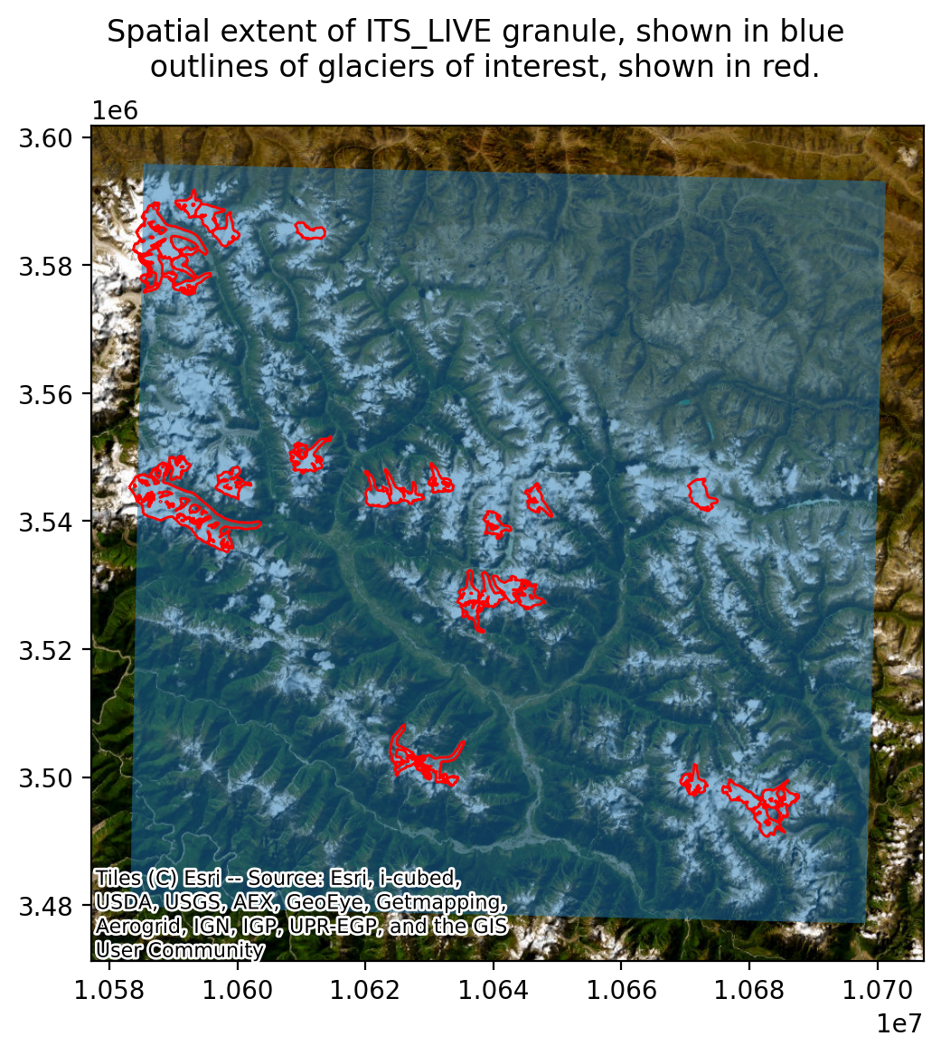
To explain this in more detail, we currently have a raster data cube (the ITS_LIVE time series) that covers the entire spatial footprint shown in blue below. However, the locations in which we are interested in this data are the glaciers outlined in red. Working with this data as a 3-dimensional vector cube is not a very efficient way of accessing the data at the locations shown in red.
Show code cell source Hide code cell source
fig, ax = plt.subplots(figsize=(12,6))
dc_bbox.to_crs('EPSG:3857').plot(ax=ax, alpha=0.5)
rgi_subset.to_crs('EPSG:3857').plot(ax=ax, facecolor='none', edgecolor='r')

cx.add_basemap(ax=ax, crs='EPSG:3857',
               source=cx.providers.Esri.WorldImagery,)
fig.suptitle('Spatial extent of ITS_LIVE granule, shown in blue \n outlines of glaciers of interest, shown in red.');
Instead, we use the Xvec.zonal_stats() method to convert the 3-dimensional cube to a 2-dimensional cube that has time dimesnion and a geometry dimension. Each element of the geometry dimension is a glacier from the rgi_subset dataframe.
Note
Because we are working with polygon geometries, we use zonal_stats() which performs a reduction over the area of the polygon. If our vector data was made up of point features, we could use Xvec.extract_points()
1) Make a vector data cube#
dask.config.set({"array.slicing.split_large_chunks": True})
vector_data_cube = dc_resamp.xvec.zonal_stats(rgi_subset.geometry,
                                       x_coords='x', y_coords='y',
).drop_vars('index')
vector_data_cube
<xarray.Dataset> Size: 898kB
Dimensions:                     (geometry: 28, mid_date: 154)
Coordinates:
  * mid_date                    (mid_date) datetime64[ns] 1kB 1986-09-30 ... ...
  * geometry                    (geometry) object 224B POLYGON Z ((698995.534...
Data variables: (12/48)
    M11                         (geometry, mid_date) float32 17kB dask.array<chunksize=(1, 148), meta=np.ndarray>
    M12                         (geometry, mid_date) float32 17kB dask.array<chunksize=(1, 148), meta=np.ndarray>
    chip_size_height            (geometry, mid_date) float32 17kB dask.array<chunksize=(1, 148), meta=np.ndarray>
    chip_size_width             (geometry, mid_date) float32 17kB dask.array<chunksize=(1, 148), meta=np.ndarray>
    interp_mask                 (geometry, mid_date) float32 17kB dask.array<chunksize=(1, 148), meta=np.ndarray>
    v                           (geometry, mid_date) float32 17kB dask.array<chunksize=(1, 148), meta=np.ndarray>
    ...                          ...
    vy_error_modeled            (geometry, mid_date) float32 17kB dask.array<chunksize=(28, 148), meta=np.ndarray>
    vy_error_slow               (geometry, mid_date) float32 17kB dask.array<chunksize=(28, 148), meta=np.ndarray>
    vy_error_stationary         (geometry, mid_date) float32 17kB dask.array<chunksize=(28, 148), meta=np.ndarray>
    vy_stable_shift             (geometry, mid_date) float32 17kB dask.array<chunksize=(28, 148), meta=np.ndarray>
    vy_stable_shift_slow        (geometry, mid_date) float32 17kB dask.array<chunksize=(28, 148), meta=np.ndarray>
    vy_stable_shift_stationary  (geometry, mid_date) float32 17kB dask.array<chunksize=(28, 148), meta=np.ndarray>
Indexes:
    geometry  GeometryIndex (crs=EPSG:32646)
Attributes: (12/19)
    Conventions:                CF-1.8
    GDAL_AREA_OR_POINT:         Area
    author:                     ITS_LIVE, a NASA MEaSUREs project (its-live.j...
    autoRIFT_parameter_file:    http://its-live-data.s3.amazonaws.com/autorif...
    datacube_software_version:  1.0
    date_created:               25-Sep-2023 22:00:23
    ...                         ...
    s3:                         s3://its-live-data/datacubes/v2/N30E090/ITS_L...
    skipped_granules:           s3://its-live-data/datacubes/v2/N30E090/ITS_L...
    time_standard_img1:         UTC
    time_standard_img2:         UTC
    title:                      ITS_LIVE datacube of image pair velocities
url: https://its-live-data.s3.amazonaws.com/datacu...- geometry: 28
- mid_date: 154
- mid_date(mid_date)datetime64[ns]1986-09-30 ... 2024-12-31
- description :
- midpoint of image 1 and image 2 acquisition date and time with granule's centroid longitude and latitude as microseconds
- standard_name :
- image_pair_center_date_with_time_separation
array(['1986-09-30T00:00:00.000000000', '1986-12-31T00:00:00.000000000', '1987-03-31T00:00:00.000000000', '1987-06-30T00:00:00.000000000', '1987-09-30T00:00:00.000000000', '1987-12-31T00:00:00.000000000', '1988-03-31T00:00:00.000000000', '1988-06-30T00:00:00.000000000', '1988-09-30T00:00:00.000000000', '1988-12-31T00:00:00.000000000', '1989-03-31T00:00:00.000000000', '1989-06-30T00:00:00.000000000', '1989-09-30T00:00:00.000000000', '1989-12-31T00:00:00.000000000', '1990-03-31T00:00:00.000000000', '1990-06-30T00:00:00.000000000', '1990-09-30T00:00:00.000000000', '1990-12-31T00:00:00.000000000', '1991-03-31T00:00:00.000000000', '1991-06-30T00:00:00.000000000', '1991-09-30T00:00:00.000000000', '1991-12-31T00:00:00.000000000', '1992-03-31T00:00:00.000000000', '1992-06-30T00:00:00.000000000', '1992-09-30T00:00:00.000000000', '1992-12-31T00:00:00.000000000', '1993-03-31T00:00:00.000000000', '1993-06-30T00:00:00.000000000', '1993-09-30T00:00:00.000000000', '1993-12-31T00:00:00.000000000', '1994-03-31T00:00:00.000000000', '1994-06-30T00:00:00.000000000', '1994-09-30T00:00:00.000000000', '1994-12-31T00:00:00.000000000', '1995-03-31T00:00:00.000000000', '1995-06-30T00:00:00.000000000', '1995-09-30T00:00:00.000000000', '1995-12-31T00:00:00.000000000', '1996-03-31T00:00:00.000000000', '1996-06-30T00:00:00.000000000', '1996-09-30T00:00:00.000000000', '1996-12-31T00:00:00.000000000', '1997-03-31T00:00:00.000000000', '1997-06-30T00:00:00.000000000', '1997-09-30T00:00:00.000000000', '1997-12-31T00:00:00.000000000', '1998-03-31T00:00:00.000000000', '1998-06-30T00:00:00.000000000', '1998-09-30T00:00:00.000000000', '1998-12-31T00:00:00.000000000', '1999-03-31T00:00:00.000000000', '1999-06-30T00:00:00.000000000', '1999-09-30T00:00:00.000000000', '1999-12-31T00:00:00.000000000', '2000-03-31T00:00:00.000000000', '2000-06-30T00:00:00.000000000', '2000-09-30T00:00:00.000000000', '2000-12-31T00:00:00.000000000', '2001-03-31T00:00:00.000000000', '2001-06-30T00:00:00.000000000', '2001-09-30T00:00:00.000000000', '2001-12-31T00:00:00.000000000', '2002-03-31T00:00:00.000000000', '2002-06-30T00:00:00.000000000', '2002-09-30T00:00:00.000000000', '2002-12-31T00:00:00.000000000', '2003-03-31T00:00:00.000000000', '2003-06-30T00:00:00.000000000', '2003-09-30T00:00:00.000000000', '2003-12-31T00:00:00.000000000', '2004-03-31T00:00:00.000000000', '2004-06-30T00:00:00.000000000', '2004-09-30T00:00:00.000000000', '2004-12-31T00:00:00.000000000', '2005-03-31T00:00:00.000000000', '2005-06-30T00:00:00.000000000', '2005-09-30T00:00:00.000000000', '2005-12-31T00:00:00.000000000', '2006-03-31T00:00:00.000000000', '2006-06-30T00:00:00.000000000', '2006-09-30T00:00:00.000000000', '2006-12-31T00:00:00.000000000', '2007-03-31T00:00:00.000000000', '2007-06-30T00:00:00.000000000', '2007-09-30T00:00:00.000000000', '2007-12-31T00:00:00.000000000', '2008-03-31T00:00:00.000000000', '2008-06-30T00:00:00.000000000', '2008-09-30T00:00:00.000000000', '2008-12-31T00:00:00.000000000', '2009-03-31T00:00:00.000000000', '2009-06-30T00:00:00.000000000', '2009-09-30T00:00:00.000000000', '2009-12-31T00:00:00.000000000', '2010-03-31T00:00:00.000000000', '2010-06-30T00:00:00.000000000', '2010-09-30T00:00:00.000000000', '2010-12-31T00:00:00.000000000', '2011-03-31T00:00:00.000000000', '2011-06-30T00:00:00.000000000', '2011-09-30T00:00:00.000000000', '2011-12-31T00:00:00.000000000', '2012-03-31T00:00:00.000000000', '2012-06-30T00:00:00.000000000', '2012-09-30T00:00:00.000000000', '2012-12-31T00:00:00.000000000', '2013-03-31T00:00:00.000000000', '2013-06-30T00:00:00.000000000', '2013-09-30T00:00:00.000000000', '2013-12-31T00:00:00.000000000', '2014-03-31T00:00:00.000000000', '2014-06-30T00:00:00.000000000', '2014-09-30T00:00:00.000000000', '2014-12-31T00:00:00.000000000', '2015-03-31T00:00:00.000000000', '2015-06-30T00:00:00.000000000', '2015-09-30T00:00:00.000000000', '2015-12-31T00:00:00.000000000', '2016-03-31T00:00:00.000000000', '2016-06-30T00:00:00.000000000', '2016-09-30T00:00:00.000000000', '2016-12-31T00:00:00.000000000', '2017-03-31T00:00:00.000000000', '2017-06-30T00:00:00.000000000', '2017-09-30T00:00:00.000000000', '2017-12-31T00:00:00.000000000', '2018-03-31T00:00:00.000000000', '2018-06-30T00:00:00.000000000', '2018-09-30T00:00:00.000000000', '2018-12-31T00:00:00.000000000', '2019-03-31T00:00:00.000000000', '2019-06-30T00:00:00.000000000', '2019-09-30T00:00:00.000000000', '2019-12-31T00:00:00.000000000', '2020-03-31T00:00:00.000000000', '2020-06-30T00:00:00.000000000', '2020-09-30T00:00:00.000000000', '2020-12-31T00:00:00.000000000', '2021-03-31T00:00:00.000000000', '2021-06-30T00:00:00.000000000', '2021-09-30T00:00:00.000000000', '2021-12-31T00:00:00.000000000', '2022-03-31T00:00:00.000000000', '2022-06-30T00:00:00.000000000', '2022-09-30T00:00:00.000000000', '2022-12-31T00:00:00.000000000', '2023-03-31T00:00:00.000000000', '2023-06-30T00:00:00.000000000', '2023-09-30T00:00:00.000000000', '2023-12-31T00:00:00.000000000', '2024-03-31T00:00:00.000000000', '2024-06-30T00:00:00.000000000', '2024-09-30T00:00:00.000000000', '2024-12-31T00:00:00.000000000'], dtype='datetime64[ns]') - geometry(geometry)objectPOLYGON Z ((698995.5345682467 33...
- crs :
- EPSG:32646
array([<POLYGON Z ((698995.535 3356459.046 0, 699011.214 3356559.24 0, 699107.132 3...>,
       <POLYGON Z ((705772.753 3360152.416 0, 705737.498 3360175.814 0, 705708.203 ...>,
       <POLYGON Z ((713890.435 3356601.497 0, 713890.464 3356565.678 0, 713890.491 ...>,
       <POLYGON Z ((720536.806 3361488.071 0, 720536.829 3361501.158 0, 720546.621 ...>,
       <POLYGON Z ((712706.746 3390103.661 0, 712675.598 3390058.796 0, 712637.197 ...>,
       <POLYGON Z ((709984.826 3391428.319 0, 709971.281 3391414.746 0, 709952.181 ...>,
       <POLYGON Z ((706806.619 3392874.368 0, 706803.249 3392895.042 0, 706798.266 ...>,
       <POLYGON Z ((700803.72 3387923.221 0, 700799.699 3387922.813 0, 700784.982 3...>,
       <POLYGON Z ((699976.616 3384703.408 0, 700003.14 3384716.652 0, 700034.702 3...>,
       <POLYGON Z ((705393.581 3387861.846 0, 705395.172 3387858.882 0, 705443.759 ...>,
       <POLYGON Z ((724401.155 3390534.628 0, 724369.306 3390516.44 0, 724309.907 3...>,
       <POLYGON Z ((741993.206 3356846.044 0, 742028.837 3356870.904 0, 742079.053 ...>,
       <POLYGON Z ((734365.846 3355131.554 0, 734365.879 3355143.422 0, 734365.882 ...>,
       <POLYGON Z ((734120.508 3356070.053 0, 734127.705 3356048.579 0, 734127.702 ...>,
       <POLYGON Z ((748703.435 3350793.001 0, 748705.001 3350796.142 0, 748720.569 ...>,
       <POLYGON Z ((774967.294 3356301.508 0, 774975.604 3356334.67 0, 774983.914 3...>,
       <POLYGON Z ((738384.154 3319942.486 0, 738372.898 3319976.404 0, 738350.299 ...>,
       <POLYGON Z ((738288.738 3320149.607 0, 738259.805 3320130.239 0, 738225.87 3...>,
       <POLYGON Z ((746220.191 3342057.954 0, 746213.81 3342067.461 0, 746196.059 3...>,
       <POLYGON Z ((746910.922 3341823.134 0, 746927.687 3341818.964 0, 746963.15 3...>,
       <POLYGON Z ((752292.061 3345011.224 0, 752298.779 3344995.627 0, 752320.011 ...>,
       <POLYGON Z ((753113.843 3357497.937 0, 753131.648 3357497.906 0, 753165.234 ...>,
       <POLYGON Z ((751947.042 3342128.041 0, 752004.359 3342133.24 0, 752056.376 3...>,
       <POLYGON Z ((747314.216 3341631.008 0, 747308.249 3341622.111 0, 747281.667 ...>,
       <POLYGON Z ((788789.137 3315761.396 0, 788768.679 3315775.065 0, 788742.911 ...>,
       <POLYGON Z ((788171.25 3315860.804 0, 788176.951 3315860.842 0, 788219.858 3...>,
       <POLYGON Z ((774553.433 3318172.303 0, 774550.27 3318179.103 0, 774537.001 3...>,
       <POLYGON Z ((781066.443 3316649.424 0, 781060.784 3316678.238 0, 781051.879 ...>],
      dtype=object)
- M11(geometry, mid_date)float32dask.array<chunksize=(1, 148), meta=np.ndarray>
- description :
- conversion matrix element (1st row, 1st column) that can be multiplied with vx to give range pixel displacement dr (see Eq. A18 in https://www.mdpi.com/2072-4292/13/4/749)
- grid_mapping :
- mapping
- standard_name :
- conversion_matrix_element_11
- units :
- pixel/(meter/year)
Array Chunk Bytes 16.84 kiB 592 B Shape (28, 154) (1, 148) Dask graph 56 chunks in 15 graph layers Data type float32 numpy.ndarray - M12(geometry, mid_date)float32dask.array<chunksize=(1, 148), meta=np.ndarray>
- description :
- conversion matrix element (1st row, 2nd column) that can be multiplied with vy to give range pixel displacement dr (see Eq. A18 in https://www.mdpi.com/2072-4292/13/4/749)
- grid_mapping :
- mapping
- standard_name :
- conversion_matrix_element_12
- units :
- pixel/(meter/year)
Array Chunk Bytes 16.84 kiB 592 B Shape (28, 154) (1, 148) Dask graph 56 chunks in 15 graph layers Data type float32 numpy.ndarray - chip_size_height(geometry, mid_date)float32dask.array<chunksize=(1, 148), meta=np.ndarray>
- chip_size_coordinates :
- Optical data: chip_size_coordinates = 'image projection geometry: width = x, height = y'. Radar data: chip_size_coordinates = 'radar geometry: width = range, height = azimuth'
- description :
- height of search template (chip)
- grid_mapping :
- mapping
- standard_name :
- chip_size_height
- units :
- m
- y_pixel_size :
- 10.0
Array Chunk Bytes 16.84 kiB 592 B Shape (28, 154) (1, 148) Dask graph 56 chunks in 15 graph layers Data type float32 numpy.ndarray - chip_size_width(geometry, mid_date)float32dask.array<chunksize=(1, 148), meta=np.ndarray>
- chip_size_coordinates :
- Optical data: chip_size_coordinates = 'image projection geometry: width = x, height = y'. Radar data: chip_size_coordinates = 'radar geometry: width = range, height = azimuth'
- description :
- width of search template (chip)
- grid_mapping :
- mapping
- standard_name :
- chip_size_width
- units :
- m
- x_pixel_size :
- 10.0
Array Chunk Bytes 16.84 kiB 592 B Shape (28, 154) (1, 148) Dask graph 56 chunks in 15 graph layers Data type float32 numpy.ndarray - interp_mask(geometry, mid_date)float32dask.array<chunksize=(1, 148), meta=np.ndarray>
- description :
- light interpolation mask
- flag_meanings :
- measured interpolated
- flag_values :
- [0, 1]
- grid_mapping :
- mapping
- standard_name :
- interpolated_value_mask
Array Chunk Bytes 16.84 kiB 592 B Shape (28, 154) (1, 148) Dask graph 56 chunks in 15 graph layers Data type float32 numpy.ndarray - v(geometry, mid_date)float32dask.array<chunksize=(1, 148), meta=np.ndarray>
- description :
- velocity magnitude
- grid_mapping :
- mapping
- standard_name :
- land_ice_surface_velocity
- units :
- meter/year
Array Chunk Bytes 16.84 kiB 592 B Shape (28, 154) (1, 148) Dask graph 56 chunks in 15 graph layers Data type float32 numpy.ndarray - v_error(geometry, mid_date)float32dask.array<chunksize=(1, 148), meta=np.ndarray>
- description :
- velocity magnitude error
- grid_mapping :
- mapping
- standard_name :
- velocity_error
- units :
- meter/year
Array Chunk Bytes 16.84 kiB 592 B Shape (28, 154) (1, 148) Dask graph 56 chunks in 15 graph layers Data type float32 numpy.ndarray - va(geometry, mid_date)float32dask.array<chunksize=(1, 148), meta=np.ndarray>
- description :
- velocity in radar azimuth direction
- grid_mapping :
- mapping
Array Chunk Bytes 16.84 kiB 592 B Shape (28, 154) (1, 148) Dask graph 56 chunks in 15 graph layers Data type float32 numpy.ndarray - vr(geometry, mid_date)float32dask.array<chunksize=(1, 148), meta=np.ndarray>
- description :
- velocity in radar range direction
- grid_mapping :
- mapping
Array Chunk Bytes 16.84 kiB 592 B Shape (28, 154) (1, 148) Dask graph 56 chunks in 15 graph layers Data type float32 numpy.ndarray - vx(geometry, mid_date)float32dask.array<chunksize=(1, 148), meta=np.ndarray>
- description :
- velocity component in x direction
- grid_mapping :
- mapping
- standard_name :
- land_ice_surface_x_velocity
- units :
- meter/year
Array Chunk Bytes 16.84 kiB 592 B Shape (28, 154) (1, 148) Dask graph 56 chunks in 15 graph layers Data type float32 numpy.ndarray - vy(geometry, mid_date)float32dask.array<chunksize=(1, 148), meta=np.ndarray>
- description :
- velocity component in y direction
- grid_mapping :
- mapping
- standard_name :
- land_ice_surface_y_velocity
- units :
- meter/year
Array Chunk Bytes 16.84 kiB 592 B Shape (28, 154) (1, 148) Dask graph 56 chunks in 15 graph layers Data type float32 numpy.ndarray - floatingice(geometry, mid_date)float32dask.array<chunksize=(1, 154), meta=np.ndarray>
- description :
- floating ice mask, 0 = non-floating-ice, 1 = floating-ice
- flag_meanings :
- non-ice ice
- flag_values :
- [0, 1]
- grid_mapping :
- mapping
- standard_name :
- floating ice mask
- url :
- https://its-live-data.s3.amazonaws.com/autorift_parameters/v001/N46_0120m_floatingice.tif
Array Chunk Bytes 16.84 kiB 616 B Shape (28, 154) (1, 154) Dask graph 28 chunks in 10 graph layers Data type float32 numpy.ndarray - landice(geometry, mid_date)float32dask.array<chunksize=(1, 154), meta=np.ndarray>
- description :
- land ice mask, 0 = non-land-ice, 1 = land-ice
- flag_meanings :
- non-ice ice
- flag_values :
- [0, 1]
- grid_mapping :
- mapping
- standard_name :
- land ice mask
- url :
- https://its-live-data.s3.amazonaws.com/autorift_parameters/v001/N46_0120m_landice.tif
Array Chunk Bytes 16.84 kiB 616 B Shape (28, 154) (1, 154) Dask graph 28 chunks in 10 graph layers Data type float32 numpy.ndarray - M11_dr_to_vr_factor(geometry, mid_date)float32dask.array<chunksize=(28, 148), meta=np.ndarray>
- description :
- multiplicative factor that converts slant range pixel displacement dr to slant range velocity vr
- standard_name :
- M11_dr_to_vr_factor
- units :
- meter/(year*pixel)
Array Chunk Bytes 16.84 kiB 16.19 kiB Shape (28, 154) (28, 148) Dask graph 2 chunks in 7 graph layers Data type float32 numpy.ndarray - M12_dr_to_vr_factor(geometry, mid_date)float32dask.array<chunksize=(28, 148), meta=np.ndarray>
- description :
- multiplicative factor that converts slant range pixel displacement dr to slant range velocity vr
- standard_name :
- M12_dr_to_vr_factor
- units :
- meter/(year*pixel)
Array Chunk Bytes 16.84 kiB 16.19 kiB Shape (28, 154) (28, 148) Dask graph 2 chunks in 7 graph layers Data type float32 numpy.ndarray - date_dt(geometry, mid_date)timedelta64[ns]dask.array<chunksize=(28, 148), meta=np.ndarray>
- description :
- time separation between acquisition of image 1 and image 2
- standard_name :
- image_pair_time_separation
Array Chunk Bytes 33.69 kiB 32.38 kiB Shape (28, 154) (28, 148) Dask graph 2 chunks in 9 graph layers Data type timedelta64[ns] numpy.ndarray - roi_valid_percentage(geometry, mid_date)float32dask.array<chunksize=(28, 148), meta=np.ndarray>
- description :
- percentage of pixels with a valid velocity estimate determined for the intersection of the full image pair footprint and the region of interest (roi) that defines where autoRIFT tried to estimate a velocity
- standard_name :
- region_of_interest_valid_pixel_percentage
Array Chunk Bytes 16.84 kiB 16.19 kiB Shape (28, 154) (28, 148) Dask graph 2 chunks in 7 graph layers Data type float32 numpy.ndarray - stable_count_slow(geometry, mid_date)float64dask.array<chunksize=(28, 148), meta=np.ndarray>
- description :
- number of valid pixels over slowest 25% of ice
- standard_name :
- stable_count_slow
- units :
- count
Array Chunk Bytes 33.69 kiB 32.38 kiB Shape (28, 154) (28, 148) Dask graph 2 chunks in 7 graph layers Data type float64 numpy.ndarray - stable_count_stationary(geometry, mid_date)float64dask.array<chunksize=(28, 148), meta=np.ndarray>
- description :
- number of valid pixels over stationary or slow-flowing surfaces
- standard_name :
- stable_count_stationary
- units :
- count
Array Chunk Bytes 33.69 kiB 32.38 kiB Shape (28, 154) (28, 148) Dask graph 2 chunks in 7 graph layers Data type float64 numpy.ndarray - stable_shift_flag(geometry, mid_date)float64dask.array<chunksize=(28, 148), meta=np.ndarray>
- description :
- flag for applying velocity bias correction: 0 = no correction; 1 = correction from overlapping stable surface mask (stationary or slow-flowing surfaces with velocity < 15 m/yr)(top priority); 2 = correction from slowest 25% of overlapping velocities (second priority)
- standard_name :
- stable_shift_flag
Array Chunk Bytes 33.69 kiB 32.38 kiB Shape (28, 154) (28, 148) Dask graph 2 chunks in 7 graph layers Data type float64 numpy.ndarray - va_error(geometry, mid_date)float32dask.array<chunksize=(28, 148), meta=np.ndarray>
- description :
- error for velocity in radar azimuth direction
- standard_name :
- va_error
- units :
- meter/year
Array Chunk Bytes 16.84 kiB 16.19 kiB Shape (28, 154) (28, 148) Dask graph 2 chunks in 7 graph layers Data type float32 numpy.ndarray - va_error_modeled(geometry, mid_date)float32dask.array<chunksize=(28, 148), meta=np.ndarray>
- description :
- 1-sigma error calculated using a modeled error-dt relationship
- standard_name :
- va_error_modeled
- units :
- meter/year
Array Chunk Bytes 16.84 kiB 16.19 kiB Shape (28, 154) (28, 148) Dask graph 2 chunks in 7 graph layers Data type float32 numpy.ndarray - va_error_slow(geometry, mid_date)float32dask.array<chunksize=(28, 148), meta=np.ndarray>
- description :
- RMSE over slowest 25% of retrieved velocities
- standard_name :
- va_error_slow
- units :
- meter/year
Array Chunk Bytes 16.84 kiB 16.19 kiB Shape (28, 154) (28, 148) Dask graph 2 chunks in 7 graph layers Data type float32 numpy.ndarray - va_error_stationary(geometry, mid_date)float32dask.array<chunksize=(28, 148), meta=np.ndarray>
- description :
- RMSE over stable surfaces, stationary or slow-flowing surfaces with velocity < 15 m/yr identified from an external mask
- standard_name :
- va_error_stationary
- units :
- meter/year
Array Chunk Bytes 16.84 kiB 16.19 kiB Shape (28, 154) (28, 148) Dask graph 2 chunks in 7 graph layers Data type float32 numpy.ndarray - va_stable_shift(geometry, mid_date)float32dask.array<chunksize=(28, 148), meta=np.ndarray>
- description :
- applied va shift calibrated using pixels over stable or slow surfaces
- standard_name :
- va_stable_shift
- units :
- meter/year
Array Chunk Bytes 16.84 kiB 16.19 kiB Shape (28, 154) (28, 148) Dask graph 2 chunks in 7 graph layers Data type float32 numpy.ndarray - va_stable_shift_slow(geometry, mid_date)float32dask.array<chunksize=(28, 148), meta=np.ndarray>
- description :
- va shift calibrated using valid pixels over slowest 25% of retrieved velocities
- standard_name :
- va_stable_shift_slow
- units :
- meter/year
Array Chunk Bytes 16.84 kiB 16.19 kiB Shape (28, 154) (28, 148) Dask graph 2 chunks in 7 graph layers Data type float32 numpy.ndarray - va_stable_shift_stationary(geometry, mid_date)float32dask.array<chunksize=(28, 148), meta=np.ndarray>
- description :
- va shift calibrated using valid pixels over stable surfaces, stationary or slow-flowing surfaces with velocity < 15 m/yr identified from an external mask
- standard_name :
- va_stable_shift_stationary
- units :
- meter/year
Array Chunk Bytes 16.84 kiB 16.19 kiB Shape (28, 154) (28, 148) Dask graph 2 chunks in 7 graph layers Data type float32 numpy.ndarray - vr_error(geometry, mid_date)float32dask.array<chunksize=(28, 148), meta=np.ndarray>
- description :
- error for velocity in radar range direction
- standard_name :
- vr_error
- units :
- meter/year
Array Chunk Bytes 16.84 kiB 16.19 kiB Shape (28, 154) (28, 148) Dask graph 2 chunks in 7 graph layers Data type float32 numpy.ndarray - vr_error_modeled(geometry, mid_date)float32dask.array<chunksize=(28, 148), meta=np.ndarray>
- description :
- 1-sigma error calculated using a modeled error-dt relationship
- standard_name :
- vr_error_modeled
- units :
- meter/year
Array Chunk Bytes 16.84 kiB 16.19 kiB Shape (28, 154) (28, 148) Dask graph 2 chunks in 7 graph layers Data type float32 numpy.ndarray - vr_error_slow(geometry, mid_date)float32dask.array<chunksize=(28, 148), meta=np.ndarray>
- description :
- RMSE over slowest 25% of retrieved velocities
- standard_name :
- vr_error_slow
- units :
- meter/year
Array Chunk Bytes 16.84 kiB 16.19 kiB Shape (28, 154) (28, 148) Dask graph 2 chunks in 7 graph layers Data type float32 numpy.ndarray - vr_error_stationary(geometry, mid_date)float32dask.array<chunksize=(28, 148), meta=np.ndarray>
- description :
- RMSE over stable surfaces, stationary or slow-flowing surfaces with velocity < 15 m/yr identified from an external mask
- standard_name :
- vr_error_stationary
- units :
- meter/year
Array Chunk Bytes 16.84 kiB 16.19 kiB Shape (28, 154) (28, 148) Dask graph 2 chunks in 7 graph layers Data type float32 numpy.ndarray - vr_stable_shift(geometry, mid_date)float32dask.array<chunksize=(28, 148), meta=np.ndarray>
- description :
- applied vr shift calibrated using pixels over stable or slow surfaces
- standard_name :
- vr_stable_shift
- units :
- meter/year
Array Chunk Bytes 16.84 kiB 16.19 kiB Shape (28, 154) (28, 148) Dask graph 2 chunks in 7 graph layers Data type float32 numpy.ndarray - vr_stable_shift_slow(geometry, mid_date)float32dask.array<chunksize=(28, 148), meta=np.ndarray>
- description :
- vr shift calibrated using valid pixels over slowest 25% of retrieved velocities
- standard_name :
- vr_stable_shift_slow
- units :
- meter/year
Array Chunk Bytes 16.84 kiB 16.19 kiB Shape (28, 154) (28, 148) Dask graph 2 chunks in 7 graph layers Data type float32 numpy.ndarray - vr_stable_shift_stationary(geometry, mid_date)float32dask.array<chunksize=(28, 148), meta=np.ndarray>
- description :
- vr shift calibrated using valid pixels over stable surfaces, stationary or slow-flowing surfaces with velocity < 15 m/yr identified from an external mask
- standard_name :
- vr_stable_shift_stationary
- units :
- meter/year
Array Chunk Bytes 16.84 kiB 16.19 kiB Shape (28, 154) (28, 148) Dask graph 2 chunks in 7 graph layers Data type float32 numpy.ndarray - vx_error(geometry, mid_date)float32dask.array<chunksize=(28, 148), meta=np.ndarray>
- description :
- best estimate of x_velocity error: vx_error is populated according to the approach used for the velocity bias correction as indicated in "stable_shift_flag"
- standard_name :
- vx_error
- units :
- meter/year
Array Chunk Bytes 16.84 kiB 16.19 kiB Shape (28, 154) (28, 148) Dask graph 2 chunks in 7 graph layers Data type float32 numpy.ndarray - vx_error_modeled(geometry, mid_date)float32dask.array<chunksize=(28, 148), meta=np.ndarray>
- description :
- 1-sigma error calculated using a modeled error-dt relationship
- standard_name :
- vx_error_modeled
- units :
- meter/year
Array Chunk Bytes 16.84 kiB 16.19 kiB Shape (28, 154) (28, 148) Dask graph 2 chunks in 7 graph layers Data type float32 numpy.ndarray - vx_error_slow(geometry, mid_date)float32dask.array<chunksize=(28, 148), meta=np.ndarray>
- description :
- RMSE over slowest 25% of retrieved velocities
- standard_name :
- vx_error_slow
- units :
- meter/year
Array Chunk Bytes 16.84 kiB 16.19 kiB Shape (28, 154) (28, 148) Dask graph 2 chunks in 7 graph layers Data type float32 numpy.ndarray - vx_error_stationary(geometry, mid_date)float32dask.array<chunksize=(28, 148), meta=np.ndarray>
- description :
- RMSE over stable surfaces, stationary or slow-flowing surfaces with velocity < 15 meter/year identified from an external mask
- standard_name :
- vx_error_stationary
- units :
- meter/year
Array Chunk Bytes 16.84 kiB 16.19 kiB Shape (28, 154) (28, 148) Dask graph 2 chunks in 7 graph layers Data type float32 numpy.ndarray - vx_stable_shift(geometry, mid_date)float32dask.array<chunksize=(28, 148), meta=np.ndarray>
- description :
- applied vx shift calibrated using pixels over stable or slow surfaces
- standard_name :
- vx_stable_shift
- units :
- meter/year
Array Chunk Bytes 16.84 kiB 16.19 kiB Shape (28, 154) (28, 148) Dask graph 2 chunks in 7 graph layers Data type float32 numpy.ndarray - vx_stable_shift_slow(geometry, mid_date)float32dask.array<chunksize=(28, 148), meta=np.ndarray>
- description :
- vx shift calibrated using valid pixels over slowest 25% of retrieved velocities
- standard_name :
- vx_stable_shift_slow
- units :
- meter/year
Array Chunk Bytes 16.84 kiB 16.19 kiB Shape (28, 154) (28, 148) Dask graph 2 chunks in 7 graph layers Data type float32 numpy.ndarray - vx_stable_shift_stationary(geometry, mid_date)float32dask.array<chunksize=(28, 148), meta=np.ndarray>
- description :
- vx shift calibrated using valid pixels over stable surfaces, stationary or slow-flowing surfaces with velocity < 15 m/yr identified from an external mask
- standard_name :
- vx_stable_shift_stationary
- units :
- meter/year
Array Chunk Bytes 16.84 kiB 16.19 kiB Shape (28, 154) (28, 148) Dask graph 2 chunks in 7 graph layers Data type float32 numpy.ndarray - vy_error(geometry, mid_date)float32dask.array<chunksize=(28, 148), meta=np.ndarray>
- description :
- best estimate of y_velocity error: vy_error is populated according to the approach used for the velocity bias correction as indicated in "stable_shift_flag"
- standard_name :
- vy_error
- units :
- meter/year
Array Chunk Bytes 16.84 kiB 16.19 kiB Shape (28, 154) (28, 148) Dask graph 2 chunks in 7 graph layers Data type float32 numpy.ndarray - vy_error_modeled(geometry, mid_date)float32dask.array<chunksize=(28, 148), meta=np.ndarray>
- description :
- 1-sigma error calculated using a modeled error-dt relationship
- standard_name :
- vy_error_modeled
- units :
- meter/year
Array Chunk Bytes 16.84 kiB 16.19 kiB Shape (28, 154) (28, 148) Dask graph 2 chunks in 7 graph layers Data type float32 numpy.ndarray - vy_error_slow(geometry, mid_date)float32dask.array<chunksize=(28, 148), meta=np.ndarray>
- description :
- RMSE over slowest 25% of retrieved velocities
- standard_name :
- vy_error_slow
- units :
- meter/year
Array Chunk Bytes 16.84 kiB 16.19 kiB Shape (28, 154) (28, 148) Dask graph 2 chunks in 7 graph layers Data type float32 numpy.ndarray - vy_error_stationary(geometry, mid_date)float32dask.array<chunksize=(28, 148), meta=np.ndarray>
- description :
- RMSE over stable surfaces, stationary or slow-flowing surfaces with velocity < 15 meter/year identified from an external mask
- standard_name :
- vy_error_stationary
- units :
- meter/year
Array Chunk Bytes 16.84 kiB 16.19 kiB Shape (28, 154) (28, 148) Dask graph 2 chunks in 7 graph layers Data type float32 numpy.ndarray - vy_stable_shift(geometry, mid_date)float32dask.array<chunksize=(28, 148), meta=np.ndarray>
- description :
- applied vy shift calibrated using pixels over stable or slow surfaces
- standard_name :
- vy_stable_shift
- units :
- meter/year
Array Chunk Bytes 16.84 kiB 16.19 kiB Shape (28, 154) (28, 148) Dask graph 2 chunks in 7 graph layers Data type float32 numpy.ndarray - vy_stable_shift_slow(geometry, mid_date)float32dask.array<chunksize=(28, 148), meta=np.ndarray>
- description :
- vy shift calibrated using valid pixels over slowest 25% of retrieved velocities
- standard_name :
- vy_stable_shift_slow
- units :
- meter/year
Array Chunk Bytes 16.84 kiB 16.19 kiB Shape (28, 154) (28, 148) Dask graph 2 chunks in 7 graph layers Data type float32 numpy.ndarray - vy_stable_shift_stationary(geometry, mid_date)float32dask.array<chunksize=(28, 148), meta=np.ndarray>
- description :
- vy shift calibrated using valid pixels over stable surfaces, stationary or slow-flowing surfaces with velocity < 15 m/yr identified from an external mask
- standard_name :
- vy_stable_shift_stationary
- units :
- meter/year
Array Chunk Bytes 16.84 kiB 16.19 kiB Shape (28, 154) (28, 148) Dask graph 2 chunks in 7 graph layers Data type float32 numpy.ndarray
- mid_datePandasIndex
PandasIndex(DatetimeIndex(['1986-09-30', '1986-12-31', '1987-03-31', '1987-06-30', '1987-09-30', '1987-12-31', '1988-03-31', '1988-06-30', '1988-09-30', '1988-12-31', ... '2022-09-30', '2022-12-31', '2023-03-31', '2023-06-30', '2023-09-30', '2023-12-31', '2024-03-31', '2024-06-30', '2024-09-30', '2024-12-31'], dtype='datetime64[ns]', name='mid_date', length=154, freq='3ME')) - geometryGeometryIndex (crs=EPSG:32646)
GeometryIndex(
    [<POLYGON Z ((698995.535 3356459.046 0, 699011.214 3356559.24 0, 699107.132 3...>
     <POLYGON Z ((705772.753 3360152.416 0, 705737.498 3360175.814 0, 705708.203 ...>
     <POLYGON Z ((713890.435 3356601.497 0, 713890.464 3356565.678 0, 713890.491 ...>
     <POLYGON Z ((720536.806 3361488.071 0, 720536.829 3361501.158 0, 720546.621 ...>
     ...
     <POLYGON Z ((788789.137 3315761.396 0, 788768.679 3315775.065 0, 788742.911 ...>
     <POLYGON Z ((788171.25 3315860.804 0, 788176.951 3315860.842 0, 788219.858 3...>
     <POLYGON Z ((774553.433 3318172.303 0, 774550.27 3318179.103 0, 774537.001 3...>
     <POLYGON Z ((781066.443 3316649.424 0, 781060.784 3316678.238 0, 781051.879 ...>],
    crs=EPSG:32646)
- Conventions :
- CF-1.8
- GDAL_AREA_OR_POINT :
- Area
- author :
- ITS_LIVE, a NASA MEaSUREs project (its-live.jpl.nasa.gov)
- autoRIFT_parameter_file :
- http://its-live-data.s3.amazonaws.com/autorift_parameters/v001/autorift_landice_0120m.shp
- datacube_software_version :
- 1.0
- date_created :
- 25-Sep-2023 22:00:23
- date_updated :
- 13-Nov-2024 00:08:07
- geo_polygon :
- [[95.06959008486952, 29.814255053135895], [95.32812062059084, 29.809951334550703], [95.58659184122865, 29.80514261876954], [95.84499718862224, 29.7998293459177], [96.10333011481168, 29.79401200205343], [96.11032804508507, 30.019297601073085], [96.11740568350054, 30.244573983323825], [96.12456379063154, 30.469841094022847], [96.1318031397002, 30.695098878594504], [95.87110827645229, 30.70112924501256], [95.61033817656023, 30.7066371044805], [95.34949964126946, 30.711621947056347], [95.08859948278467, 30.716083310981194], [95.08376623410525, 30.49063893600811], [95.07898726183609, 30.26518607254204], [95.0742620484426, 30.039724763743482], [95.06959008486952, 29.814255053135895]]
- institution :
- NASA Jet Propulsion Laboratory (JPL), California Institute of Technology
- latitude :
- 30.26
- longitude :
- 95.6
- proj_polygon :
- [[700000, 3300000], [725000.0, 3300000.0], [750000.0, 3300000.0], [775000.0, 3300000.0], [800000, 3300000], [800000.0, 3325000.0], [800000.0, 3350000.0], [800000.0, 3375000.0], [800000, 3400000], [775000.0, 3400000.0], [750000.0, 3400000.0], [725000.0, 3400000.0], [700000, 3400000], [700000.0, 3375000.0], [700000.0, 3350000.0], [700000.0, 3325000.0], [700000, 3300000]]
- projection :
- 32646
- s3 :
- s3://its-live-data/datacubes/v2/N30E090/ITS_LIVE_vel_EPSG32646_G0120_X750000_Y3350000.zarr
- skipped_granules :
- s3://its-live-data/datacubes/v2/N30E090/ITS_LIVE_vel_EPSG32646_G0120_X750000_Y3350000.json
- time_standard_img1 :
- UTC
- time_standard_img2 :
- UTC
- title :
- ITS_LIVE datacube of image pair velocities
- url :
- https://its-live-data.s3.amazonaws.com/datacubes/v2/N30E090/ITS_LIVE_vel_EPSG32646_G0120_X750000_Y3350000.zarr
Great, now we’ve gone from a 3-d object with (mid_date,x,y) dimensions to a 2-d object with (mid_date, geometry) dimensions. However, in addition to the geometry data stored in the vector dataframe, we’d also like to add some of the attribute data to the ITS_LIVE time series vector cube. The following cell adds attributes as coordinate variables to the vector data cube.
2) Add attribute data to vector cube#
#Define attributes to be added
rgi_attrs_dict = {'RGIId': 'rgi_id',
              'Area_km2': 'area_km2',
              'Slope_deg': 'slope_deg'}

def update_cube_attrs(ds, gdf, attrs_dict):
    for k, v in attrs_dict.items():
        ds[k] = (('geometry'), gdf[v].values)
        ds = ds.assign_coords({k: ds[k]})
    return ds

vector_data_cube = update_cube_attrs(vector_data_cube, rgi_subset, rgi_attrs_dict)
vector_data_cube
<xarray.Dataset> Size: 899kB
Dimensions:                     (geometry: 28, mid_date: 154)
Coordinates:
  * mid_date                    (mid_date) datetime64[ns] 1kB 1986-09-30 ... ...
  * geometry                    (geometry) object 224B POLYGON Z ((698995.534...
    RGIId                       (geometry) object 224B 'RGI2000-v7.0-G-15-116...
    Area_km2                    (geometry) float64 224B 60.49 5.03 ... 8.753
    Slope_deg                   (geometry) float64 224B 21.73 19.25 ... 17.63
Data variables: (12/48)
    M11                         (geometry, mid_date) float32 17kB dask.array<chunksize=(1, 148), meta=np.ndarray>
    M12                         (geometry, mid_date) float32 17kB dask.array<chunksize=(1, 148), meta=np.ndarray>
    chip_size_height            (geometry, mid_date) float32 17kB dask.array<chunksize=(1, 148), meta=np.ndarray>
    chip_size_width             (geometry, mid_date) float32 17kB dask.array<chunksize=(1, 148), meta=np.ndarray>
    interp_mask                 (geometry, mid_date) float32 17kB dask.array<chunksize=(1, 148), meta=np.ndarray>
    v                           (geometry, mid_date) float32 17kB dask.array<chunksize=(1, 148), meta=np.ndarray>
    ...                          ...
    vy_error_modeled            (geometry, mid_date) float32 17kB dask.array<chunksize=(28, 148), meta=np.ndarray>
    vy_error_slow               (geometry, mid_date) float32 17kB dask.array<chunksize=(28, 148), meta=np.ndarray>
    vy_error_stationary         (geometry, mid_date) float32 17kB dask.array<chunksize=(28, 148), meta=np.ndarray>
    vy_stable_shift             (geometry, mid_date) float32 17kB dask.array<chunksize=(28, 148), meta=np.ndarray>
    vy_stable_shift_slow        (geometry, mid_date) float32 17kB dask.array<chunksize=(28, 148), meta=np.ndarray>
    vy_stable_shift_stationary  (geometry, mid_date) float32 17kB dask.array<chunksize=(28, 148), meta=np.ndarray>
Indexes:
    geometry  GeometryIndex (crs=EPSG:32646)
Attributes: (12/19)
    Conventions:                CF-1.8
    GDAL_AREA_OR_POINT:         Area
    author:                     ITS_LIVE, a NASA MEaSUREs project (its-live.j...
    autoRIFT_parameter_file:    http://its-live-data.s3.amazonaws.com/autorif...
    datacube_software_version:  1.0
    date_created:               25-Sep-2023 22:00:23
    ...                         ...
    s3:                         s3://its-live-data/datacubes/v2/N30E090/ITS_L...
    skipped_granules:           s3://its-live-data/datacubes/v2/N30E090/ITS_L...
    time_standard_img1:         UTC
    time_standard_img2:         UTC
    title:                      ITS_LIVE datacube of image pair velocities
url: https://its-live-data.s3.amazonaws.com/datacu...- geometry: 28
- mid_date: 154
- mid_date(mid_date)datetime64[ns]1986-09-30 ... 2024-12-31
- description :
- midpoint of image 1 and image 2 acquisition date and time with granule's centroid longitude and latitude as microseconds
- standard_name :
- image_pair_center_date_with_time_separation
array(['1986-09-30T00:00:00.000000000', '1986-12-31T00:00:00.000000000', '1987-03-31T00:00:00.000000000', '1987-06-30T00:00:00.000000000', '1987-09-30T00:00:00.000000000', '1987-12-31T00:00:00.000000000', '1988-03-31T00:00:00.000000000', '1988-06-30T00:00:00.000000000', '1988-09-30T00:00:00.000000000', '1988-12-31T00:00:00.000000000', '1989-03-31T00:00:00.000000000', '1989-06-30T00:00:00.000000000', '1989-09-30T00:00:00.000000000', '1989-12-31T00:00:00.000000000', '1990-03-31T00:00:00.000000000', '1990-06-30T00:00:00.000000000', '1990-09-30T00:00:00.000000000', '1990-12-31T00:00:00.000000000', '1991-03-31T00:00:00.000000000', '1991-06-30T00:00:00.000000000', '1991-09-30T00:00:00.000000000', '1991-12-31T00:00:00.000000000', '1992-03-31T00:00:00.000000000', '1992-06-30T00:00:00.000000000', '1992-09-30T00:00:00.000000000', '1992-12-31T00:00:00.000000000', '1993-03-31T00:00:00.000000000', '1993-06-30T00:00:00.000000000', '1993-09-30T00:00:00.000000000', '1993-12-31T00:00:00.000000000', '1994-03-31T00:00:00.000000000', '1994-06-30T00:00:00.000000000', '1994-09-30T00:00:00.000000000', '1994-12-31T00:00:00.000000000', '1995-03-31T00:00:00.000000000', '1995-06-30T00:00:00.000000000', '1995-09-30T00:00:00.000000000', '1995-12-31T00:00:00.000000000', '1996-03-31T00:00:00.000000000', '1996-06-30T00:00:00.000000000', '1996-09-30T00:00:00.000000000', '1996-12-31T00:00:00.000000000', '1997-03-31T00:00:00.000000000', '1997-06-30T00:00:00.000000000', '1997-09-30T00:00:00.000000000', '1997-12-31T00:00:00.000000000', '1998-03-31T00:00:00.000000000', '1998-06-30T00:00:00.000000000', '1998-09-30T00:00:00.000000000', '1998-12-31T00:00:00.000000000', '1999-03-31T00:00:00.000000000', '1999-06-30T00:00:00.000000000', '1999-09-30T00:00:00.000000000', '1999-12-31T00:00:00.000000000', '2000-03-31T00:00:00.000000000', '2000-06-30T00:00:00.000000000', '2000-09-30T00:00:00.000000000', '2000-12-31T00:00:00.000000000', '2001-03-31T00:00:00.000000000', '2001-06-30T00:00:00.000000000', '2001-09-30T00:00:00.000000000', '2001-12-31T00:00:00.000000000', '2002-03-31T00:00:00.000000000', '2002-06-30T00:00:00.000000000', '2002-09-30T00:00:00.000000000', '2002-12-31T00:00:00.000000000', '2003-03-31T00:00:00.000000000', '2003-06-30T00:00:00.000000000', '2003-09-30T00:00:00.000000000', '2003-12-31T00:00:00.000000000', '2004-03-31T00:00:00.000000000', '2004-06-30T00:00:00.000000000', '2004-09-30T00:00:00.000000000', '2004-12-31T00:00:00.000000000', '2005-03-31T00:00:00.000000000', '2005-06-30T00:00:00.000000000', '2005-09-30T00:00:00.000000000', '2005-12-31T00:00:00.000000000', '2006-03-31T00:00:00.000000000', '2006-06-30T00:00:00.000000000', '2006-09-30T00:00:00.000000000', '2006-12-31T00:00:00.000000000', '2007-03-31T00:00:00.000000000', '2007-06-30T00:00:00.000000000', '2007-09-30T00:00:00.000000000', '2007-12-31T00:00:00.000000000', '2008-03-31T00:00:00.000000000', '2008-06-30T00:00:00.000000000', '2008-09-30T00:00:00.000000000', '2008-12-31T00:00:00.000000000', '2009-03-31T00:00:00.000000000', '2009-06-30T00:00:00.000000000', '2009-09-30T00:00:00.000000000', '2009-12-31T00:00:00.000000000', '2010-03-31T00:00:00.000000000', '2010-06-30T00:00:00.000000000', '2010-09-30T00:00:00.000000000', '2010-12-31T00:00:00.000000000', '2011-03-31T00:00:00.000000000', '2011-06-30T00:00:00.000000000', '2011-09-30T00:00:00.000000000', '2011-12-31T00:00:00.000000000', '2012-03-31T00:00:00.000000000', '2012-06-30T00:00:00.000000000', '2012-09-30T00:00:00.000000000', '2012-12-31T00:00:00.000000000', '2013-03-31T00:00:00.000000000', '2013-06-30T00:00:00.000000000', '2013-09-30T00:00:00.000000000', '2013-12-31T00:00:00.000000000', '2014-03-31T00:00:00.000000000', '2014-06-30T00:00:00.000000000', '2014-09-30T00:00:00.000000000', '2014-12-31T00:00:00.000000000', '2015-03-31T00:00:00.000000000', '2015-06-30T00:00:00.000000000', '2015-09-30T00:00:00.000000000', '2015-12-31T00:00:00.000000000', '2016-03-31T00:00:00.000000000', '2016-06-30T00:00:00.000000000', '2016-09-30T00:00:00.000000000', '2016-12-31T00:00:00.000000000', '2017-03-31T00:00:00.000000000', '2017-06-30T00:00:00.000000000', '2017-09-30T00:00:00.000000000', '2017-12-31T00:00:00.000000000', '2018-03-31T00:00:00.000000000', '2018-06-30T00:00:00.000000000', '2018-09-30T00:00:00.000000000', '2018-12-31T00:00:00.000000000', '2019-03-31T00:00:00.000000000', '2019-06-30T00:00:00.000000000', '2019-09-30T00:00:00.000000000', '2019-12-31T00:00:00.000000000', '2020-03-31T00:00:00.000000000', '2020-06-30T00:00:00.000000000', '2020-09-30T00:00:00.000000000', '2020-12-31T00:00:00.000000000', '2021-03-31T00:00:00.000000000', '2021-06-30T00:00:00.000000000', '2021-09-30T00:00:00.000000000', '2021-12-31T00:00:00.000000000', '2022-03-31T00:00:00.000000000', '2022-06-30T00:00:00.000000000', '2022-09-30T00:00:00.000000000', '2022-12-31T00:00:00.000000000', '2023-03-31T00:00:00.000000000', '2023-06-30T00:00:00.000000000', '2023-09-30T00:00:00.000000000', '2023-12-31T00:00:00.000000000', '2024-03-31T00:00:00.000000000', '2024-06-30T00:00:00.000000000', '2024-09-30T00:00:00.000000000', '2024-12-31T00:00:00.000000000'], dtype='datetime64[ns]') - geometry(geometry)objectPOLYGON Z ((698995.5345682467 33...
- crs :
- EPSG:32646
array([<POLYGON Z ((698995.535 3356459.046 0, 699011.214 3356559.24 0, 699107.132 3...>, <POLYGON Z ((705772.753 3360152.416 0, 705737.498 3360175.814 0, 705708.203 ...>, <POLYGON Z ((713890.435 3356601.497 0, 713890.464 3356565.678 0, 713890.491 ...>, <POLYGON Z ((720536.806 3361488.071 0, 720536.829 3361501.158 0, 720546.621 ...>, <POLYGON Z ((712706.746 3390103.661 0, 712675.598 3390058.796 0, 712637.197 ...>, <POLYGON Z ((709984.826 3391428.319 0, 709971.281 3391414.746 0, 709952.181 ...>, <POLYGON Z ((706806.619 3392874.368 0, 706803.249 3392895.042 0, 706798.266 ...>, <POLYGON Z ((700803.72 3387923.221 0, 700799.699 3387922.813 0, 700784.982 3...>, <POLYGON Z ((699976.616 3384703.408 0, 700003.14 3384716.652 0, 700034.702 3...>, <POLYGON Z ((705393.581 3387861.846 0, 705395.172 3387858.882 0, 705443.759 ...>, <POLYGON Z ((724401.155 3390534.628 0, 724369.306 3390516.44 0, 724309.907 3...>, <POLYGON Z ((741993.206 3356846.044 0, 742028.837 3356870.904 0, 742079.053 ...>, <POLYGON Z ((734365.846 3355131.554 0, 734365.879 3355143.422 0, 734365.882 ...>, <POLYGON Z ((734120.508 3356070.053 0, 734127.705 3356048.579 0, 734127.702 ...>, <POLYGON Z ((748703.435 3350793.001 0, 748705.001 3350796.142 0, 748720.569 ...>, <POLYGON Z ((774967.294 3356301.508 0, 774975.604 3356334.67 0, 774983.914 3...>, <POLYGON Z ((738384.154 3319942.486 0, 738372.898 3319976.404 0, 738350.299 ...>, <POLYGON Z ((738288.738 3320149.607 0, 738259.805 3320130.239 0, 738225.87 3...>, <POLYGON Z ((746220.191 3342057.954 0, 746213.81 3342067.461 0, 746196.059 3...>, <POLYGON Z ((746910.922 3341823.134 0, 746927.687 3341818.964 0, 746963.15 3...>, <POLYGON Z ((752292.061 3345011.224 0, 752298.779 3344995.627 0, 752320.011 ...>, <POLYGON Z ((753113.843 3357497.937 0, 753131.648 3357497.906 0, 753165.234 ...>, <POLYGON Z ((751947.042 3342128.041 0, 752004.359 3342133.24 0, 752056.376 3...>, <POLYGON Z ((747314.216 3341631.008 0, 747308.249 3341622.111 0, 747281.667 ...>, <POLYGON Z ((788789.137 3315761.396 0, 788768.679 3315775.065 0, 788742.911 ...>, <POLYGON Z ((788171.25 3315860.804 0, 788176.951 3315860.842 0, 788219.858 3...>, <POLYGON Z ((774553.433 3318172.303 0, 774550.27 3318179.103 0, 774537.001 3...>, <POLYGON Z ((781066.443 3316649.424 0, 781060.784 3316678.238 0, 781051.879 ...>], dtype=object) - RGIId(geometry)object'RGI2000-v7.0-G-15-11631' ... 'R...
array(['RGI2000-v7.0-G-15-11631', 'RGI2000-v7.0-G-15-11632', 'RGI2000-v7.0-G-15-11643', 'RGI2000-v7.0-G-15-11673', 'RGI2000-v7.0-G-15-11736', 'RGI2000-v7.0-G-15-11740', 'RGI2000-v7.0-G-15-11746', 'RGI2000-v7.0-G-15-11754', 'RGI2000-v7.0-G-15-11759', 'RGI2000-v7.0-G-15-11766', 'RGI2000-v7.0-G-15-11895', 'RGI2000-v7.0-G-15-11985', 'RGI2000-v7.0-G-15-11994', 'RGI2000-v7.0-G-15-11995', 'RGI2000-v7.0-G-15-12015', 'RGI2000-v7.0-G-15-12194', 'RGI2000-v7.0-G-15-15962', 'RGI2000-v7.0-G-15-15966', 'RGI2000-v7.0-G-15-16033', 'RGI2000-v7.0-G-15-16035', 'RGI2000-v7.0-G-15-16036', 'RGI2000-v7.0-G-15-16076', 'RGI2000-v7.0-G-15-16108', 'RGI2000-v7.0-G-15-16116', 'RGI2000-v7.0-G-15-16255', 'RGI2000-v7.0-G-15-16257', 'RGI2000-v7.0-G-15-16408', 'RGI2000-v7.0-G-15-16461'], dtype=object) - Area_km2(geometry)float6460.49 5.03 9.064 ... 6.347 8.753
array([60.48661959, 5.0298586 , 9.06411693, 11.14699277, 6.87766255, 7.14607431, 5.26094339, 30.27183227, 10.4203802 , 8.8574929 , 5.28957485, 5.56885407, 7.65952778, 7.99324513, 5.73005761, 8.797407 , 10.75042324, 7.43202273, 6.11020999, 6.76472928, 7.27440259, 6.1395563 , 6.34673974, 5.40041877, 7.75420555, 10.1584097 , 6.34670755, 8.75300401]) - Slope_deg(geometry)float6421.73 19.25 23.26 ... 23.99 17.63
array([21.731916, 19.250132, 23.261293, 20.035536, 14.739693, 13.551242,
       18.288933, 16.769985, 20.0946  , 20.302011, 16.508911, 20.586494,
       23.91235 , 28.171831, 23.489735, 12.372513, 27.019384, 26.973549,
       23.651398, 21.954998, 19.140688, 18.677023, 22.96521 , 27.2453  ,
       25.916887, 22.803406, 23.990732, 17.626614])
- M11(geometry, mid_date)float32dask.array<chunksize=(1, 148), meta=np.ndarray>
- description :
- conversion matrix element (1st row, 1st column) that can be multiplied with vx to give range pixel displacement dr (see Eq. A18 in https://www.mdpi.com/2072-4292/13/4/749)
- grid_mapping :
- mapping
- standard_name :
- conversion_matrix_element_11
- units :
- pixel/(meter/year)
Array Chunk Bytes 16.84 kiB 592 B Shape (28, 154) (1, 148) Dask graph 56 chunks in 15 graph layers Data type float32 numpy.ndarray - M12(geometry, mid_date)float32dask.array<chunksize=(1, 148), meta=np.ndarray>
- description :
- conversion matrix element (1st row, 2nd column) that can be multiplied with vy to give range pixel displacement dr (see Eq. A18 in https://www.mdpi.com/2072-4292/13/4/749)
- grid_mapping :
- mapping
- standard_name :
- conversion_matrix_element_12
- units :
- pixel/(meter/year)
Array Chunk Bytes 16.84 kiB 592 B Shape (28, 154) (1, 148) Dask graph 56 chunks in 15 graph layers Data type float32 numpy.ndarray - chip_size_height(geometry, mid_date)float32dask.array<chunksize=(1, 148), meta=np.ndarray>
- chip_size_coordinates :
- Optical data: chip_size_coordinates = 'image projection geometry: width = x, height = y'. Radar data: chip_size_coordinates = 'radar geometry: width = range, height = azimuth'
- description :
- height of search template (chip)
- grid_mapping :
- mapping
- standard_name :
- chip_size_height
- units :
- m
- y_pixel_size :
- 10.0
Array Chunk Bytes 16.84 kiB 592 B Shape (28, 154) (1, 148) Dask graph 56 chunks in 15 graph layers Data type float32 numpy.ndarray - chip_size_width(geometry, mid_date)float32dask.array<chunksize=(1, 148), meta=np.ndarray>
- chip_size_coordinates :
- Optical data: chip_size_coordinates = 'image projection geometry: width = x, height = y'. Radar data: chip_size_coordinates = 'radar geometry: width = range, height = azimuth'
- description :
- width of search template (chip)
- grid_mapping :
- mapping
- standard_name :
- chip_size_width
- units :
- m
- x_pixel_size :
- 10.0
Array Chunk Bytes 16.84 kiB 592 B Shape (28, 154) (1, 148) Dask graph 56 chunks in 15 graph layers Data type float32 numpy.ndarray - interp_mask(geometry, mid_date)float32dask.array<chunksize=(1, 148), meta=np.ndarray>
- description :
- light interpolation mask
- flag_meanings :
- measured interpolated
- flag_values :
- [0, 1]
- grid_mapping :
- mapping
- standard_name :
- interpolated_value_mask
Array Chunk Bytes 16.84 kiB 592 B Shape (28, 154) (1, 148) Dask graph 56 chunks in 15 graph layers Data type float32 numpy.ndarray - v(geometry, mid_date)float32dask.array<chunksize=(1, 148), meta=np.ndarray>
- description :
- velocity magnitude
- grid_mapping :
- mapping
- standard_name :
- land_ice_surface_velocity
- units :
- meter/year
Array Chunk Bytes 16.84 kiB 592 B Shape (28, 154) (1, 148) Dask graph 56 chunks in 15 graph layers Data type float32 numpy.ndarray - v_error(geometry, mid_date)float32dask.array<chunksize=(1, 148), meta=np.ndarray>
- description :
- velocity magnitude error
- grid_mapping :
- mapping
- standard_name :
- velocity_error
- units :
- meter/year
Array Chunk Bytes 16.84 kiB 592 B Shape (28, 154) (1, 148) Dask graph 56 chunks in 15 graph layers Data type float32 numpy.ndarray - va(geometry, mid_date)float32dask.array<chunksize=(1, 148), meta=np.ndarray>
- description :
- velocity in radar azimuth direction
- grid_mapping :
- mapping
Array Chunk Bytes 16.84 kiB 592 B Shape (28, 154) (1, 148) Dask graph 56 chunks in 15 graph layers Data type float32 numpy.ndarray - vr(geometry, mid_date)float32dask.array<chunksize=(1, 148), meta=np.ndarray>
- description :
- velocity in radar range direction
- grid_mapping :
- mapping
Array Chunk Bytes 16.84 kiB 592 B Shape (28, 154) (1, 148) Dask graph 56 chunks in 15 graph layers Data type float32 numpy.ndarray - vx(geometry, mid_date)float32dask.array<chunksize=(1, 148), meta=np.ndarray>
- description :
- velocity component in x direction
- grid_mapping :
- mapping
- standard_name :
- land_ice_surface_x_velocity
- units :
- meter/year
Array Chunk Bytes 16.84 kiB 592 B Shape (28, 154) (1, 148) Dask graph 56 chunks in 15 graph layers Data type float32 numpy.ndarray - vy(geometry, mid_date)float32dask.array<chunksize=(1, 148), meta=np.ndarray>
- description :
- velocity component in y direction
- grid_mapping :
- mapping
- standard_name :
- land_ice_surface_y_velocity
- units :
- meter/year
Array Chunk Bytes 16.84 kiB 592 B Shape (28, 154) (1, 148) Dask graph 56 chunks in 15 graph layers Data type float32 numpy.ndarray - floatingice(geometry, mid_date)float32dask.array<chunksize=(1, 154), meta=np.ndarray>
- description :
- floating ice mask, 0 = non-floating-ice, 1 = floating-ice
- flag_meanings :
- non-ice ice
- flag_values :
- [0, 1]
- grid_mapping :
- mapping
- standard_name :
- floating ice mask
- url :
- https://its-live-data.s3.amazonaws.com/autorift_parameters/v001/N46_0120m_floatingice.tif
Array Chunk Bytes 16.84 kiB 616 B Shape (28, 154) (1, 154) Dask graph 28 chunks in 10 graph layers Data type float32 numpy.ndarray - landice(geometry, mid_date)float32dask.array<chunksize=(1, 154), meta=np.ndarray>
- description :
- land ice mask, 0 = non-land-ice, 1 = land-ice
- flag_meanings :
- non-ice ice
- flag_values :
- [0, 1]
- grid_mapping :
- mapping
- standard_name :
- land ice mask
- url :
- https://its-live-data.s3.amazonaws.com/autorift_parameters/v001/N46_0120m_landice.tif
Array Chunk Bytes 16.84 kiB 616 B Shape (28, 154) (1, 154) Dask graph 28 chunks in 10 graph layers Data type float32 numpy.ndarray - M11_dr_to_vr_factor(geometry, mid_date)float32dask.array<chunksize=(28, 148), meta=np.ndarray>
- description :
- multiplicative factor that converts slant range pixel displacement dr to slant range velocity vr
- standard_name :
- M11_dr_to_vr_factor
- units :
- meter/(year*pixel)
Array Chunk Bytes 16.84 kiB 16.19 kiB Shape (28, 154) (28, 148) Dask graph 2 chunks in 7 graph layers Data type float32 numpy.ndarray - M12_dr_to_vr_factor(geometry, mid_date)float32dask.array<chunksize=(28, 148), meta=np.ndarray>
- description :
- multiplicative factor that converts slant range pixel displacement dr to slant range velocity vr
- standard_name :
- M12_dr_to_vr_factor
- units :
- meter/(year*pixel)
Array Chunk Bytes 16.84 kiB 16.19 kiB Shape (28, 154) (28, 148) Dask graph 2 chunks in 7 graph layers Data type float32 numpy.ndarray - date_dt(geometry, mid_date)timedelta64[ns]dask.array<chunksize=(28, 148), meta=np.ndarray>
- description :
- time separation between acquisition of image 1 and image 2
- standard_name :
- image_pair_time_separation
Array Chunk Bytes 33.69 kiB 32.38 kiB Shape (28, 154) (28, 148) Dask graph 2 chunks in 9 graph layers Data type timedelta64[ns] numpy.ndarray - roi_valid_percentage(geometry, mid_date)float32dask.array<chunksize=(28, 148), meta=np.ndarray>
- description :
- percentage of pixels with a valid velocity estimate determined for the intersection of the full image pair footprint and the region of interest (roi) that defines where autoRIFT tried to estimate a velocity
- standard_name :
- region_of_interest_valid_pixel_percentage
Array Chunk Bytes 16.84 kiB 16.19 kiB Shape (28, 154) (28, 148) Dask graph 2 chunks in 7 graph layers Data type float32 numpy.ndarray - stable_count_slow(geometry, mid_date)float64dask.array<chunksize=(28, 148), meta=np.ndarray>
- description :
- number of valid pixels over slowest 25% of ice
- standard_name :
- stable_count_slow
- units :
- count
Array Chunk Bytes 33.69 kiB 32.38 kiB Shape (28, 154) (28, 148) Dask graph 2 chunks in 7 graph layers Data type float64 numpy.ndarray - stable_count_stationary(geometry, mid_date)float64dask.array<chunksize=(28, 148), meta=np.ndarray>
- description :
- number of valid pixels over stationary or slow-flowing surfaces
- standard_name :
- stable_count_stationary
- units :
- count
Array Chunk Bytes 33.69 kiB 32.38 kiB Shape (28, 154) (28, 148) Dask graph 2 chunks in 7 graph layers Data type float64 numpy.ndarray - stable_shift_flag(geometry, mid_date)float64dask.array<chunksize=(28, 148), meta=np.ndarray>
- description :
- flag for applying velocity bias correction: 0 = no correction; 1 = correction from overlapping stable surface mask (stationary or slow-flowing surfaces with velocity < 15 m/yr)(top priority); 2 = correction from slowest 25% of overlapping velocities (second priority)
- standard_name :
- stable_shift_flag
Array Chunk Bytes 33.69 kiB 32.38 kiB Shape (28, 154) (28, 148) Dask graph 2 chunks in 7 graph layers Data type float64 numpy.ndarray - va_error(geometry, mid_date)float32dask.array<chunksize=(28, 148), meta=np.ndarray>
- description :
- error for velocity in radar azimuth direction
- standard_name :
- va_error
- units :
- meter/year
Array Chunk Bytes 16.84 kiB 16.19 kiB Shape (28, 154) (28, 148) Dask graph 2 chunks in 7 graph layers Data type float32 numpy.ndarray - va_error_modeled(geometry, mid_date)float32dask.array<chunksize=(28, 148), meta=np.ndarray>
- description :
- 1-sigma error calculated using a modeled error-dt relationship
- standard_name :
- va_error_modeled
- units :
- meter/year
Array Chunk Bytes 16.84 kiB 16.19 kiB Shape (28, 154) (28, 148) Dask graph 2 chunks in 7 graph layers Data type float32 numpy.ndarray - va_error_slow(geometry, mid_date)float32dask.array<chunksize=(28, 148), meta=np.ndarray>
- description :
- RMSE over slowest 25% of retrieved velocities
- standard_name :
- va_error_slow
- units :
- meter/year
Array Chunk Bytes 16.84 kiB 16.19 kiB Shape (28, 154) (28, 148) Dask graph 2 chunks in 7 graph layers Data type float32 numpy.ndarray - va_error_stationary(geometry, mid_date)float32dask.array<chunksize=(28, 148), meta=np.ndarray>
- description :
- RMSE over stable surfaces, stationary or slow-flowing surfaces with velocity < 15 m/yr identified from an external mask
- standard_name :
- va_error_stationary
- units :
- meter/year
Array Chunk Bytes 16.84 kiB 16.19 kiB Shape (28, 154) (28, 148) Dask graph 2 chunks in 7 graph layers Data type float32 numpy.ndarray - va_stable_shift(geometry, mid_date)float32dask.array<chunksize=(28, 148), meta=np.ndarray>
- description :
- applied va shift calibrated using pixels over stable or slow surfaces
- standard_name :
- va_stable_shift
- units :
- meter/year
Array Chunk Bytes 16.84 kiB 16.19 kiB Shape (28, 154) (28, 148) Dask graph 2 chunks in 7 graph layers Data type float32 numpy.ndarray - va_stable_shift_slow(geometry, mid_date)float32dask.array<chunksize=(28, 148), meta=np.ndarray>
- description :
- va shift calibrated using valid pixels over slowest 25% of retrieved velocities
- standard_name :
- va_stable_shift_slow
- units :
- meter/year
Array Chunk Bytes 16.84 kiB 16.19 kiB Shape (28, 154) (28, 148) Dask graph 2 chunks in 7 graph layers Data type float32 numpy.ndarray - va_stable_shift_stationary(geometry, mid_date)float32dask.array<chunksize=(28, 148), meta=np.ndarray>
- description :
- va shift calibrated using valid pixels over stable surfaces, stationary or slow-flowing surfaces with velocity < 15 m/yr identified from an external mask
- standard_name :
- va_stable_shift_stationary
- units :
- meter/year
Array Chunk Bytes 16.84 kiB 16.19 kiB Shape (28, 154) (28, 148) Dask graph 2 chunks in 7 graph layers Data type float32 numpy.ndarray - vr_error(geometry, mid_date)float32dask.array<chunksize=(28, 148), meta=np.ndarray>
- description :
- error for velocity in radar range direction
- standard_name :
- vr_error
- units :
- meter/year
Array Chunk Bytes 16.84 kiB 16.19 kiB Shape (28, 154) (28, 148) Dask graph 2 chunks in 7 graph layers Data type float32 numpy.ndarray - vr_error_modeled(geometry, mid_date)float32dask.array<chunksize=(28, 148), meta=np.ndarray>
- description :
- 1-sigma error calculated using a modeled error-dt relationship
- standard_name :
- vr_error_modeled
- units :
- meter/year
Array Chunk Bytes 16.84 kiB 16.19 kiB Shape (28, 154) (28, 148) Dask graph 2 chunks in 7 graph layers Data type float32 numpy.ndarray - vr_error_slow(geometry, mid_date)float32dask.array<chunksize=(28, 148), meta=np.ndarray>
- description :
- RMSE over slowest 25% of retrieved velocities
- standard_name :
- vr_error_slow
- units :
- meter/year
Array Chunk Bytes 16.84 kiB 16.19 kiB Shape (28, 154) (28, 148) Dask graph 2 chunks in 7 graph layers Data type float32 numpy.ndarray - vr_error_stationary(geometry, mid_date)float32dask.array<chunksize=(28, 148), meta=np.ndarray>
- description :
- RMSE over stable surfaces, stationary or slow-flowing surfaces with velocity < 15 m/yr identified from an external mask
- standard_name :
- vr_error_stationary
- units :
- meter/year
Array Chunk Bytes 16.84 kiB 16.19 kiB Shape (28, 154) (28, 148) Dask graph 2 chunks in 7 graph layers Data type float32 numpy.ndarray - vr_stable_shift(geometry, mid_date)float32dask.array<chunksize=(28, 148), meta=np.ndarray>
- description :
- applied vr shift calibrated using pixels over stable or slow surfaces
- standard_name :
- vr_stable_shift
- units :
- meter/year
Array Chunk Bytes 16.84 kiB 16.19 kiB Shape (28, 154) (28, 148) Dask graph 2 chunks in 7 graph layers Data type float32 numpy.ndarray - vr_stable_shift_slow(geometry, mid_date)float32dask.array<chunksize=(28, 148), meta=np.ndarray>
- description :
- vr shift calibrated using valid pixels over slowest 25% of retrieved velocities
- standard_name :
- vr_stable_shift_slow
- units :
- meter/year
Array Chunk Bytes 16.84 kiB 16.19 kiB Shape (28, 154) (28, 148) Dask graph 2 chunks in 7 graph layers Data type float32 numpy.ndarray - vr_stable_shift_stationary(geometry, mid_date)float32dask.array<chunksize=(28, 148), meta=np.ndarray>
- description :
- vr shift calibrated using valid pixels over stable surfaces, stationary or slow-flowing surfaces with velocity < 15 m/yr identified from an external mask
- standard_name :
- vr_stable_shift_stationary
- units :
- meter/year
Array Chunk Bytes 16.84 kiB 16.19 kiB Shape (28, 154) (28, 148) Dask graph 2 chunks in 7 graph layers Data type float32 numpy.ndarray - vx_error(geometry, mid_date)float32dask.array<chunksize=(28, 148), meta=np.ndarray>
- description :
- best estimate of x_velocity error: vx_error is populated according to the approach used for the velocity bias correction as indicated in "stable_shift_flag"
- standard_name :
- vx_error
- units :
- meter/year
Array Chunk Bytes 16.84 kiB 16.19 kiB Shape (28, 154) (28, 148) Dask graph 2 chunks in 7 graph layers Data type float32 numpy.ndarray - vx_error_modeled(geometry, mid_date)float32dask.array<chunksize=(28, 148), meta=np.ndarray>
- description :
- 1-sigma error calculated using a modeled error-dt relationship
- standard_name :
- vx_error_modeled
- units :
- meter/year
Array Chunk Bytes 16.84 kiB 16.19 kiB Shape (28, 154) (28, 148) Dask graph 2 chunks in 7 graph layers Data type float32 numpy.ndarray - vx_error_slow(geometry, mid_date)float32dask.array<chunksize=(28, 148), meta=np.ndarray>
- description :
- RMSE over slowest 25% of retrieved velocities
- standard_name :
- vx_error_slow
- units :
- meter/year
Array Chunk Bytes 16.84 kiB 16.19 kiB Shape (28, 154) (28, 148) Dask graph 2 chunks in 7 graph layers Data type float32 numpy.ndarray - vx_error_stationary(geometry, mid_date)float32dask.array<chunksize=(28, 148), meta=np.ndarray>
- description :
- RMSE over stable surfaces, stationary or slow-flowing surfaces with velocity < 15 meter/year identified from an external mask
- standard_name :
- vx_error_stationary
- units :
- meter/year
Array Chunk Bytes 16.84 kiB 16.19 kiB Shape (28, 154) (28, 148) Dask graph 2 chunks in 7 graph layers Data type float32 numpy.ndarray - vx_stable_shift(geometry, mid_date)float32dask.array<chunksize=(28, 148), meta=np.ndarray>
- description :
- applied vx shift calibrated using pixels over stable or slow surfaces
- standard_name :
- vx_stable_shift
- units :
- meter/year
Array Chunk Bytes 16.84 kiB 16.19 kiB Shape (28, 154) (28, 148) Dask graph 2 chunks in 7 graph layers Data type float32 numpy.ndarray - vx_stable_shift_slow(geometry, mid_date)float32dask.array<chunksize=(28, 148), meta=np.ndarray>
- description :
- vx shift calibrated using valid pixels over slowest 25% of retrieved velocities
- standard_name :
- vx_stable_shift_slow
- units :
- meter/year
Array Chunk Bytes 16.84 kiB 16.19 kiB Shape (28, 154) (28, 148) Dask graph 2 chunks in 7 graph layers Data type float32 numpy.ndarray - vx_stable_shift_stationary(geometry, mid_date)float32dask.array<chunksize=(28, 148), meta=np.ndarray>
- description :
- vx shift calibrated using valid pixels over stable surfaces, stationary or slow-flowing surfaces with velocity < 15 m/yr identified from an external mask
- standard_name :
- vx_stable_shift_stationary
- units :
- meter/year
Array Chunk Bytes 16.84 kiB 16.19 kiB Shape (28, 154) (28, 148) Dask graph 2 chunks in 7 graph layers Data type float32 numpy.ndarray - vy_error(geometry, mid_date)float32dask.array<chunksize=(28, 148), meta=np.ndarray>
- description :
- best estimate of y_velocity error: vy_error is populated according to the approach used for the velocity bias correction as indicated in "stable_shift_flag"
- standard_name :
- vy_error
- units :
- meter/year
Array Chunk Bytes 16.84 kiB 16.19 kiB Shape (28, 154) (28, 148) Dask graph 2 chunks in 7 graph layers Data type float32 numpy.ndarray - vy_error_modeled(geometry, mid_date)float32dask.array<chunksize=(28, 148), meta=np.ndarray>
- description :
- 1-sigma error calculated using a modeled error-dt relationship
- standard_name :
- vy_error_modeled
- units :
- meter/year
Array Chunk Bytes 16.84 kiB 16.19 kiB Shape (28, 154) (28, 148) Dask graph 2 chunks in 7 graph layers Data type float32 numpy.ndarray - vy_error_slow(geometry, mid_date)float32dask.array<chunksize=(28, 148), meta=np.ndarray>
- description :
- RMSE over slowest 25% of retrieved velocities
- standard_name :
- vy_error_slow
- units :
- meter/year
Array Chunk Bytes 16.84 kiB 16.19 kiB Shape (28, 154) (28, 148) Dask graph 2 chunks in 7 graph layers Data type float32 numpy.ndarray - vy_error_stationary(geometry, mid_date)float32dask.array<chunksize=(28, 148), meta=np.ndarray>
- description :
- RMSE over stable surfaces, stationary or slow-flowing surfaces with velocity < 15 meter/year identified from an external mask
- standard_name :
- vy_error_stationary
- units :
- meter/year
Array Chunk Bytes 16.84 kiB 16.19 kiB Shape (28, 154) (28, 148) Dask graph 2 chunks in 7 graph layers Data type float32 numpy.ndarray - vy_stable_shift(geometry, mid_date)float32dask.array<chunksize=(28, 148), meta=np.ndarray>
- description :
- applied vy shift calibrated using pixels over stable or slow surfaces
- standard_name :
- vy_stable_shift
- units :
- meter/year
Array Chunk Bytes 16.84 kiB 16.19 kiB Shape (28, 154) (28, 148) Dask graph 2 chunks in 7 graph layers Data type float32 numpy.ndarray - vy_stable_shift_slow(geometry, mid_date)float32dask.array<chunksize=(28, 148), meta=np.ndarray>
- description :
- vy shift calibrated using valid pixels over slowest 25% of retrieved velocities
- standard_name :
- vy_stable_shift_slow
- units :
- meter/year
Array Chunk Bytes 16.84 kiB 16.19 kiB Shape (28, 154) (28, 148) Dask graph 2 chunks in 7 graph layers Data type float32 numpy.ndarray - vy_stable_shift_stationary(geometry, mid_date)float32dask.array<chunksize=(28, 148), meta=np.ndarray>
- description :
- vy shift calibrated using valid pixels over stable surfaces, stationary or slow-flowing surfaces with velocity < 15 m/yr identified from an external mask
- standard_name :
- vy_stable_shift_stationary
- units :
- meter/year
Array Chunk Bytes 16.84 kiB 16.19 kiB Shape (28, 154) (28, 148) Dask graph 2 chunks in 7 graph layers Data type float32 numpy.ndarray
- mid_datePandasIndex
PandasIndex(DatetimeIndex(['1986-09-30', '1986-12-31', '1987-03-31', '1987-06-30', '1987-09-30', '1987-12-31', '1988-03-31', '1988-06-30', '1988-09-30', '1988-12-31', ... '2022-09-30', '2022-12-31', '2023-03-31', '2023-06-30', '2023-09-30', '2023-12-31', '2024-03-31', '2024-06-30', '2024-09-30', '2024-12-31'], dtype='datetime64[ns]', name='mid_date', length=154, freq='3ME')) - geometryGeometryIndex (crs=EPSG:32646)
GeometryIndex(
    [<POLYGON Z ((698995.535 3356459.046 0, 699011.214 3356559.24 0, 699107.132 3...>
     <POLYGON Z ((705772.753 3360152.416 0, 705737.498 3360175.814 0, 705708.203 ...>
     <POLYGON Z ((713890.435 3356601.497 0, 713890.464 3356565.678 0, 713890.491 ...>
     <POLYGON Z ((720536.806 3361488.071 0, 720536.829 3361501.158 0, 720546.621 ...>
     ...
     <POLYGON Z ((788789.137 3315761.396 0, 788768.679 3315775.065 0, 788742.911 ...>
     <POLYGON Z ((788171.25 3315860.804 0, 788176.951 3315860.842 0, 788219.858 3...>
     <POLYGON Z ((774553.433 3318172.303 0, 774550.27 3318179.103 0, 774537.001 3...>
     <POLYGON Z ((781066.443 3316649.424 0, 781060.784 3316678.238 0, 781051.879 ...>],
    crs=EPSG:32646)
- Conventions :
- CF-1.8
- GDAL_AREA_OR_POINT :
- Area
- author :
- ITS_LIVE, a NASA MEaSUREs project (its-live.jpl.nasa.gov)
- autoRIFT_parameter_file :
- http://its-live-data.s3.amazonaws.com/autorift_parameters/v001/autorift_landice_0120m.shp
- datacube_software_version :
- 1.0
- date_created :
- 25-Sep-2023 22:00:23
- date_updated :
- 13-Nov-2024 00:08:07
- geo_polygon :
- [[95.06959008486952, 29.814255053135895], [95.32812062059084, 29.809951334550703], [95.58659184122865, 29.80514261876954], [95.84499718862224, 29.7998293459177], [96.10333011481168, 29.79401200205343], [96.11032804508507, 30.019297601073085], [96.11740568350054, 30.244573983323825], [96.12456379063154, 30.469841094022847], [96.1318031397002, 30.695098878594504], [95.87110827645229, 30.70112924501256], [95.61033817656023, 30.7066371044805], [95.34949964126946, 30.711621947056347], [95.08859948278467, 30.716083310981194], [95.08376623410525, 30.49063893600811], [95.07898726183609, 30.26518607254204], [95.0742620484426, 30.039724763743482], [95.06959008486952, 29.814255053135895]]
- institution :
- NASA Jet Propulsion Laboratory (JPL), California Institute of Technology
- latitude :
- 30.26
- longitude :
- 95.6
- proj_polygon :
- [[700000, 3300000], [725000.0, 3300000.0], [750000.0, 3300000.0], [775000.0, 3300000.0], [800000, 3300000], [800000.0, 3325000.0], [800000.0, 3350000.0], [800000.0, 3375000.0], [800000, 3400000], [775000.0, 3400000.0], [750000.0, 3400000.0], [725000.0, 3400000.0], [700000, 3400000], [700000.0, 3375000.0], [700000.0, 3350000.0], [700000.0, 3325000.0], [700000, 3300000]]
- projection :
- 32646
- s3 :
- s3://its-live-data/datacubes/v2/N30E090/ITS_LIVE_vel_EPSG32646_G0120_X750000_Y3350000.zarr
- skipped_granules :
- s3://its-live-data/datacubes/v2/N30E090/ITS_LIVE_vel_EPSG32646_G0120_X750000_Y3350000.json
- time_standard_img1 :
- UTC
- time_standard_img2 :
- UTC
- title :
- ITS_LIVE datacube of image pair velocities
- url :
- https://its-live-data.s3.amazonaws.com/datacubes/v2/N30E090/ITS_LIVE_vel_EPSG32646_G0120_X750000_Y3350000.zarr
3) Write vector cube to disk#
Later in this notebook, we will want to perform operations that require this object to be loaded into memory. All of our steps thus far have happened lazily, and when we do load the data into memory it will be quite time-consuming.
To skip this step, I’ve loaded the data into memory and written it to disk. This allows us to read the vector data cube (which is much more manageable) into memory from file.
Because this step is quite computationally intensive, I won’t execute it here, but I will include the code for the sake of completeness.
Steps to write vector data cube to disk#
Encode vector data code geometries as [CF] geometries. This is required because Shapely geometries (how geometries are represented in memory) are not compatible with array-based file formats such as Zarr. To get around this, Xvec uses a package called cf-xarray to encode the Shapely geometries as CF geometries. For more detail on reading and writing vector data cubes, see the Xvec documentation.
encoded_vdc = vector_data_cube.xvec.encode_cf()
Write encoded data cube to Zarr (This triggers
.compute(), loading the data into memory before writing it to disk. On my computer, this took about 12 minutes.with ProgressBar(): encoded_vdc.to_zarr('data/regional_glacier_velocity_vector_cube.zarr', mode='w')
Output: [########################################] | 100% Completed | 12m 15s
C. Data visualization#
1) Read vector data cube into memory#
The vector data cube is stored on disk with CF geometries. We go through the reverse of the process we used to write the object to disk, decoding the CF geometries to Shapely geometries with xvec.decode_cf().
vector_data_cube_cf = xr.open_zarr('../data/regional_glacier_velocity_vector_cube.zarr')
vector_data_cube = vector_data_cube_cf.xvec.decode_cf().compute()
2) Visualize velocity data#
Xvec has a method, to_geodataframe() that allows us to easily convert the xr.Dataset vector cube to a gpd.GeoDataFrame. We can then use the GeoPandas .explore() method to interactively visualize the data.
We will look at mean velocities over time.
vector_data_cube_mean = vector_data_cube.mean(dim='mid_date')

vector_data_cube_mean['vmag'] = np.sqrt(vector_data_cube_mean['vx']**2 + vector_data_cube_mean['vy']**2)

vector_data_cube_mean['vmag'].xvec.to_geodataframe(geometry='geometry').explore('vmag')
We could also look at single seasons:
vector_cube_seasonal_mean = vector_data_cube.groupby('mid_date.season').mean()

vector_cube_seasonal_mean['vmag'] = np.sqrt(vector_cube_seasonal_mean['vx']**2 + vector_cube_seasonal_mean['vy']**2)

vector_cube_seasonal_mean.sel(season='JJA')['vmag'].xvec.to_geodataframe(geometry='geometry').explore('vmag')
3) Visualize associations between velocity and attribute data#
In addition to using GeoPandas plotting features, we can still use Xarray’s built in plotting features to visualize the non-spatial elements of the data. Below, we visualize the relationships between magnitude of velocity (y-axis), glacier slope (x-axis) and glacier area (hue).
fig, ax = plt.subplots()

fig.suptitle('Mean velocity in the context of glacier area and slope', fontsize=16)

sc = vector_data_cube_mean.plot.scatter(
    x = 'Slope_deg', y='vmag', hue='Area_km2',
    ax=ax, add_colorbar=True, cbar_kwargs={'label': 'Glacier area (sq. km.)'})
ax.set_ylabel('Magnitude of velocity (m/yr)', fontsize=14)
ax.set_xlabel('Glacier slope (degrees)', fontsize=14);
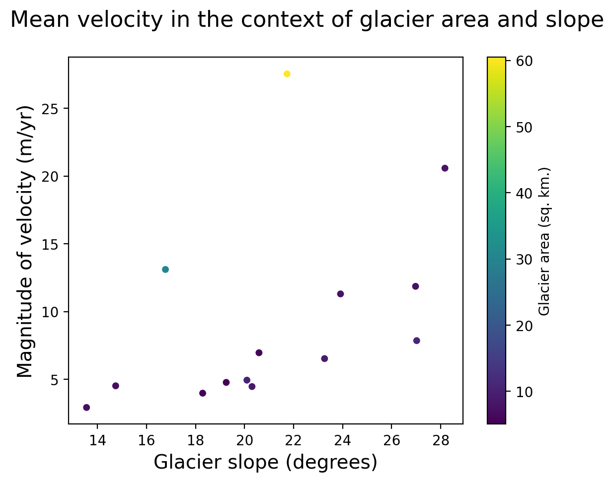
{{conclusion}}
NameError: name 'conclusion' is not defined