2. Data organization and manipulation
Introduction
This notebook illustrates initial steps involved in working with a large raster dataset (the ITS_LIVE granule that we read in the previous notebook) and subsetting it to the spatial domain of a smaller area of interest. To clip ITS_LIVE data to the extent of a single glacier, we use a vector dataset of glacier outlines, the Randolph Glacier Inventory.
We work through challenges that come with working with larger-than-memory datasets and complex geometries. The tools we will use include xarray, dask, rioxarray, geopandas, and flox.
Outline
A. Read and organize gridded ice velocity (raster) data
Compare approaches for reading larger-than-memory data
Arrange dataset in chronological order
B. Incorporate glacier outline (vector) data
Read and reproject vector data
Crop vector data to spatial extent of raster data
Optional: Handle different geometry types when visualizing vector data
C. Join raster and vector data - single glacier
Crop ITS_LIVE granule to a single glacier outline
Write clipped object to file
Learning goals
Concepts
Characteristics of larger than memory gridded data
‘Lazy’ v. ‘non-lazy’ operations
Troubleshooting code errors and warnings
Techniques
Read + write large data with Xarray, Zarr, and Dask
Label-based indexing and selection
Interactive visualizations with Folium and GeoPandas
Clip raster data with vector data using Rioxarray
Expand the next cell to see specific packages used in this notebook and relevant system and version information.
Show code cell source
%xmode minimal
from dask.distributed import Client, LocalCluster
import folium
import geopandas as gpd
import inspect
import matplotlib.pyplot as plt
import numpy as np
import pandas as pd
import rioxarray as rx
from shapely.geometry import MultiPolygon, Point, Polygon
import warnings
import xarray as xr
warnings.simplefilter(action='ignore', category=FutureWarning)
Exception reporting mode: Minimal
A. Read and organize gridded ice velocity (raster) data#
This section uses functions we defined in the data access notebook, all of which are stored in the itslivetools.py file. If you cloned this tutorial from its github repository you’ll see that itslivetools.py is in the same directory as our current notebook, so we can import it with the following line:
import itslivetools
Read in the catalog again, and use the find_granule_by_point() to find the URL that points to the ITS_LIVE granule covering your area of interest.
itslive_catalog = gpd.read_file('https://its-live-data.s3.amazonaws.com/datacubes/catalog_v02.json')
#Find urls for granule covering point of interest
url = itslivetools.find_granule_by_point([95.180191, 30.645973])
url
'http://its-live-data.s3.amazonaws.com/datacubes/v2-updated-october2024/N30E090/ITS_LIVE_vel_EPSG32646_G0120_X750000_Y3350000.zarr'
1) Compare approaches for reading larger-than-memory data#
Compare approaches for reading larger-than-memory data
The function that we defined in the previous notebook, read_in_s3(), supports different options for reading large, chunked raster datasets. Before we use that again in this notebook, we will explore these options and the ways that they can impact how we work with the data. You can learn more about reading Zarr data with Xarray here, and see the different chunking options that are supported and which we will demonstrate below here.
Chunks = 'auto'#
This is the default option in read_in_s3(). The Xarray documentation states that chunks='auto' uses “dask auto chunking, taking into account the engine preferred chunks”.
dc_auto = xr.open_dataset(url, engine='zarr', chunks='auto')
In this instance, the chunks of the object created with xr.open_dataset(..., chunks='auo') do not exactly match the chunk size
dc_auto
<xarray.Dataset> Size: 1TB
Dimensions: (mid_date: 47892, y: 833, x: 833)
Coordinates:
* mid_date (mid_date) datetime64[ns] 383kB 2022-06-07T04...
* x (x) float64 7kB 7.001e+05 7.003e+05 ... 8e+05
* y (y) float64 7kB 3.4e+06 3.4e+06 ... 3.3e+06
Data variables: (12/60)
M11 (mid_date, y, x) float32 133GB dask.array<chunksize=(47892, 20, 20), meta=np.ndarray>
M11_dr_to_vr_factor (mid_date) float32 192kB dask.array<chunksize=(47892,), meta=np.ndarray>
M12 (mid_date, y, x) float32 133GB dask.array<chunksize=(47892, 20, 20), meta=np.ndarray>
M12_dr_to_vr_factor (mid_date) float32 192kB dask.array<chunksize=(47892,), meta=np.ndarray>
acquisition_date_img1 (mid_date) datetime64[ns] 383kB dask.array<chunksize=(47892,), meta=np.ndarray>
acquisition_date_img2 (mid_date) datetime64[ns] 383kB dask.array<chunksize=(47892,), meta=np.ndarray>
... ...
vy_error_modeled (mid_date) float32 192kB dask.array<chunksize=(47892,), meta=np.ndarray>
vy_error_slow (mid_date) float32 192kB dask.array<chunksize=(47892,), meta=np.ndarray>
vy_error_stationary (mid_date) float32 192kB dask.array<chunksize=(47892,), meta=np.ndarray>
vy_stable_shift (mid_date) float32 192kB dask.array<chunksize=(47892,), meta=np.ndarray>
vy_stable_shift_slow (mid_date) float32 192kB dask.array<chunksize=(47892,), meta=np.ndarray>
vy_stable_shift_stationary (mid_date) float32 192kB dask.array<chunksize=(47892,), meta=np.ndarray>
Attributes: (12/19)
Conventions: CF-1.8
GDAL_AREA_OR_POINT: Area
author: ITS_LIVE, a NASA MEaSUREs project (its-live.j...
autoRIFT_parameter_file: http://its-live-data.s3.amazonaws.com/autorif...
datacube_software_version: 1.0
date_created: 25-Sep-2023 22:00:23
... ...
s3: s3://its-live-data/datacubes/v2/N30E090/ITS_L...
skipped_granules: s3://its-live-data/datacubes/v2/N30E090/ITS_L...
time_standard_img1: UTC
time_standard_img2: UTC
title: ITS_LIVE datacube of image pair velocities
url: https://its-live-data.s3.amazonaws.com/datacu...The data model section/notebook discussed scalar information that is stored as attributes attached to Xarray objects. Similarly, Xarray objects read from Zarr datacubes have associated encodings that tell Xarray how to read and write the object to disk. We can use the encoding to learn about preferred chunking schemes.
dc_auto['v'].encoding
{'chunks': (20000, 10, 10),
'preferred_chunks': {'mid_date': 20000, 'y': 10, 'x': 10},
'compressor': Blosc(cname='zlib', clevel=2, shuffle=SHUFFLE, blocksize=0),
'filters': None,
'missing_value': -32767,
'dtype': dtype('int16')}
dc_auto['v']
<xarray.DataArray 'v' (mid_date: 47892, y: 833, x: 833)> Size: 133GB
dask.array<open_dataset-v, shape=(47892, 833, 833), dtype=float32, chunksize=(47892, 20, 20), chunktype=numpy.ndarray>
Coordinates:
* mid_date (mid_date) datetime64[ns] 383kB 2022-06-07T04:21:44.211208960 ....
* x (x) float64 7kB 7.001e+05 7.003e+05 7.004e+05 ... 7.999e+05 8e+05
* y (y) float64 7kB 3.4e+06 3.4e+06 3.4e+06 ... 3.3e+06 3.3e+06
Attributes:
description: velocity magnitude
grid_mapping: mapping
standard_name: land_ice_surface_velocity
units: meter/yearFor the encoding of the v variable, it looks like the chunking scheme is expected to be {'mid_date': 2000, 'y':10, 'x':10}. However, the chunks for this variable created with chunks='auto' are {'mid_date': 47892, 'y': 20, 'x': 20}.
Let’s take a look at the encoding for a 1-dimensional variable:
dc_auto['vx_error']
<xarray.DataArray 'vx_error' (mid_date: 47892)> Size: 192kB
dask.array<open_dataset-vx_error, shape=(47892,), dtype=float32, chunksize=(47892,), chunktype=numpy.ndarray>
Coordinates:
* mid_date (mid_date) datetime64[ns] 383kB 2022-06-07T04:21:44.211208960 ....
Attributes:
description: best estimate of x_velocity error: vx_error is populated ...
standard_name: vx_error
units: meter/yeardc_auto['vx_error'].encoding
{'chunks': (56147,),
'preferred_chunks': {'mid_date': 56147},
'compressor': Blosc(cname='zlib', clevel=2, shuffle=SHUFFLE, blocksize=0),
'filters': None,
'_FillValue': -32767.0,
'dtype': dtype('float32')}
Interesting. We see that:
The chunk size specified in the encoding doesn’t match the total length of the
mid_datedimension. It may be an artifact from an earlier step in the data processing chain before some observations were eliminated.The encoding specifies a single chunk along the
mid_datedimension for this variable, which matches the object we read into memory, the size of this chunk is just different.
Another thing to note is that it looks like some of the variables within this xr.Dataset have different chunk sizes on the y dimension (Shown by the error produced below). We will need to address this later before rechunking the dataset.
dc_auto.chunksizes
ValueError: Object has inconsistent chunks along dimension y. This can be fixed by calling unify_chunks().
dc_auto = dc_auto.unify_chunks()
dc_auto.chunksizes
Frozen({'mid_date': (32736, 15156), 'y': (20, 20, 20, 20, 20, 20, 20, 20, 20, 20, 20, 20, 20, 20, 20, 20, 20, 20, 20, 20, 20, 20, 20, 20, 20, 20, 20, 20, 20, 20, 20, 20, 20, 20, 20, 20, 20, 20, 20, 20, 20, 13), 'x': (20, 20, 20, 20, 20, 20, 20, 20, 20, 20, 20, 20, 20, 20, 20, 20, 20, 20, 20, 20, 20, 20, 20, 20, 20, 20, 20, 20, 20, 20, 20, 20, 20, 20, 20, 20, 20, 20, 20, 20, 20, 13)})
Chunks = {}#
For this argument, the documentation says: “loads the data with dask using the engine’s preferred chunk size, generally identical to the format’s chunk size. If not available, a single chunk for all arrays.”
Note that with this dataset, 'auto' and {} don’t return the same chunking scheme.
dc_set = xr.open_dataset(url, engine='zarr', chunks={})
dc_set['v'].encoding
{'chunks': (20000, 10, 10),
'preferred_chunks': {'mid_date': 20000, 'y': 10, 'x': 10},
'compressor': Blosc(cname='zlib', clevel=2, shuffle=SHUFFLE, blocksize=0),
'filters': None,
'missing_value': -32767,
'dtype': dtype('int16')}
dc_set['v']
<xarray.DataArray 'v' (mid_date: 47892, y: 833, x: 833)> Size: 133GB
dask.array<open_dataset-v, shape=(47892, 833, 833), dtype=float32, chunksize=(20000, 10, 10), chunktype=numpy.ndarray>
Coordinates:
* mid_date (mid_date) datetime64[ns] 383kB 2022-06-07T04:21:44.211208960 ....
* x (x) float64 7kB 7.001e+05 7.003e+05 7.004e+05 ... 7.999e+05 8e+05
* y (y) float64 7kB 3.4e+06 3.4e+06 3.4e+06 ... 3.3e+06 3.3e+06
Attributes:
description: velocity magnitude
grid_mapping: mapping
standard_name: land_ice_surface_velocity
units: meter/yearWith this approach, we see that the chunking on the 3-dimensional variable we looked at above (‘v’) does match the chunking specified in the object’s encoding: {'mid_date': 20000, 'y': 10, 'x': 10}.
Looking at a one-dimensional variable, we see the same occurrence as with dc_auto: the number of chunks matches what is specified in the encoding, but the size of the chunk is different.
dc_set['vx_error'].encoding
{'chunks': (56147,),
'preferred_chunks': {'mid_date': 56147},
'compressor': Blosc(cname='zlib', clevel=2, shuffle=SHUFFLE, blocksize=0),
'filters': None,
'_FillValue': -32767.0,
'dtype': dtype('float32')}
dc_set['vx_error']
<xarray.DataArray 'vx_error' (mid_date: 47892)> Size: 192kB
dask.array<open_dataset-vx_error, shape=(47892,), dtype=float32, chunksize=(47892,), chunktype=numpy.ndarray>
Coordinates:
* mid_date (mid_date) datetime64[ns] 383kB 2022-06-07T04:21:44.211208960 ....
Attributes:
description: best estimate of x_velocity error: vx_error is populated ...
standard_name: vx_error
units: meter/yearThe v and vx_error variables shown above have different chunk sizes along the mid_date dimension, so we can expect the same chunk sizes error as above, but this time for mid_date:
dc_set.chunksizes
ValueError: Object has inconsistent chunks along dimension mid_date. This can be fixed by calling unify_chunks().
However this time, if try to resolve the above error like we did for dc_auto, We get a performance warning about the number of chunks increasing by a factor of 186.
dc_set = dc_set.unify_chunks()
PerformanceWarning: Increasing number of chunks by factor of 186_, chunked_data = chunkmanager.unify_chunks(*unify_chunks_args)
An out-of-order time dimension#
When we read this dataset from the S3 bucket, we get an object where the time dimension is not in chronological order. Because the dataset is so large, fixing this is not entirely straightforward.
for element in range(5):
print(dc_set.mid_date[element].data)
2022-06-07T04:21:44.211208960
2018-04-14T04:18:49.171219968
2017-02-10T16:15:50.660901120
2022-04-03T04:19:01.211214080
2021-07-22T04:16:46.210427904
The standard approach would be calling Xarray’s .sortby() method:
dc_set = dc_set.sortby('mid_date')
Performing an operation like sorting or slicing requires the entire array to be loaded into memory; for a larage dimension like mid_date (~48,000 elements), would be very slow and/or would max out available computationall resoures.
There may be a chunking strategy that successfully allows one to sort this dataset along the mid_date dimension, but when I tried a few different re-chunking approaches, they did not work. Instead, the sucessful approach I found was a bit counterintuitive: Re-read the dataset into memory without dask. This let’s us use Xarray’s ‘lazy’ functionality; we can sort the dataset without loading it into memory. The object will still be quite large so we will chunk the data, incorporating dask, after we sort by the time dimension.
Read the dataset without Dask#
We’ll again use the read_in_s3() function, but this time passing chunks_arg = None. This is the same as running: dc = xr.open_dataset(url, engine='Zarr'). The `read_in_s3()`` signature is shown below as a reminder:
signature = inspect.signature(itslivetools.read_in_s3)
print(signature)
(http_url: str, chunks_arg: Union[NoneType, str, dict] = 'auto') -> xarray.core.dataset.Dataset
dc = itslivetools.read_in_s3(url, None)
dc
<xarray.Dataset> Size: 1TB
Dimensions: (mid_date: 47892, y: 833, x: 833)
Coordinates:
* mid_date (mid_date) datetime64[ns] 383kB 2022-06-07T04...
* x (x) float64 7kB 7.001e+05 7.003e+05 ... 8e+05
* y (y) float64 7kB 3.4e+06 3.4e+06 ... 3.3e+06
Data variables: (12/60)
M11 (mid_date, y, x) float32 133GB ...
M11_dr_to_vr_factor (mid_date) float32 192kB ...
M12 (mid_date, y, x) float32 133GB ...
M12_dr_to_vr_factor (mid_date) float32 192kB ...
acquisition_date_img1 (mid_date) datetime64[ns] 383kB ...
acquisition_date_img2 (mid_date) datetime64[ns] 383kB ...
... ...
vy_error_modeled (mid_date) float32 192kB ...
vy_error_slow (mid_date) float32 192kB ...
vy_error_stationary (mid_date) float32 192kB ...
vy_stable_shift (mid_date) float32 192kB ...
vy_stable_shift_slow (mid_date) float32 192kB ...
vy_stable_shift_stationary (mid_date) float32 192kB ...
Attributes: (12/19)
Conventions: CF-1.8
GDAL_AREA_OR_POINT: Area
author: ITS_LIVE, a NASA MEaSUREs project (its-live.j...
autoRIFT_parameter_file: http://its-live-data.s3.amazonaws.com/autorif...
datacube_software_version: 1.0
date_created: 25-Sep-2023 22:00:23
... ...
s3: s3://its-live-data/datacubes/v2/N30E090/ITS_L...
skipped_granules: s3://its-live-data/datacubes/v2/N30E090/ITS_L...
time_standard_img1: UTC
time_standard_img2: UTC
title: ITS_LIVE datacube of image pair velocities
url: https://its-live-data.s3.amazonaws.com/datacu...As we saw above, the mid_date dimension is still out of order:
for element in range(5):
print(dc.mid_date[element].data)
2022-06-07T04:21:44.211208960
2018-04-14T04:18:49.171219968
2017-02-10T16:15:50.660901120
2022-04-03T04:19:01.211214080
2021-07-22T04:16:46.210427904
2) Arrange dataset in chronological order#
Arrange dataset in chronological order
But now, we can lazily perform the .sortby() method.
dc = dc.sortby('mid_date')
for element in range(5):
print(dc.mid_date[element].data)
1986-09-11T03:31:15.003252992
1986-10-05T03:31:06.144750016
1986-10-21T03:31:34.493249984
1986-11-22T03:29:27.023556992
1986-11-30T03:29:08.710132992
Great! After some experimentation with different approaches, we have our dataset sorted in chronological order.
Convert to a dask-backed Xarray dataset#
Not passing a 'chunks' argument to xr.open_dataset() means that the Xarray object is a collection of Numpy arrays rather than Dask arrays. However, the dataset is still very large. We will need to use Dask even though we didn’t read it in with Dask. We’ll use the preferred chunking from .encoding['chunks'] to specify a chunking scheme to the object and convert the underlying arrays from Numpy to Dask.
Note
if end up adding data overview notebook, this should be moved there. in text above this note is text to keep from the passage below if it moves.
However, the dataset is still very large: there are 60 variables that exist along 1,2 or, 3 dimensions (with the exception of the mapping variable which we will discuss later), and a single 3-d variable is 123 GB. We will still need to use Dask even though we didn’t read it in as a collection of Dask arrays straight away. We will use the preferred chunk sizes we saw in the earlier objects in order to add a chunking scheme to this object and convert the numpy arrays to Dask arrays.
chunking_dict = dc_auto.chunksizes
dc_rechunk = dc.chunk(chunking_dict)
dc_rechunk.chunks
Frozen({'mid_date': (32736, 15156), 'y': (20, 20, 20, 20, 20, 20, 20, 20, 20, 20, 20, 20, 20, 20, 20, 20, 20, 20, 20, 20, 20, 20, 20, 20, 20, 20, 20, 20, 20, 20, 20, 20, 20, 20, 20, 20, 20, 20, 20, 20, 20, 13), 'x': (20, 20, 20, 20, 20, 20, 20, 20, 20, 20, 20, 20, 20, 20, 20, 20, 20, 20, 20, 20, 20, 20, 20, 20, 20, 20, 20, 20, 20, 20, 20, 20, 20, 20, 20, 20, 20, 20, 20, 20, 20, 13)})
Great, now we have our ITS_LIVE dataset organized by time, and with appropriate chunking. Let’s move on and read in vector data describing some physical features we’d like to examine with the ITS_LIVE dataset.
B. Incorporate glacier outline (vector) data#
1) Read and reproject vector data#
As discussed in the Software and Data notebook, the examples in this tutorial use glacier outlines from the Randolph Glacier Inventory, version 7 (RGI7). We’ll specifically be looking at the ‘South Asia East’ region.
se_asia = gpd.read_parquet('../data/rgi7_region15_south_asia_east.parquet')
Check the projection of the ITS_LIVE dataset, which is stored in the attributes of the dc / dc_rechunk objects.
dc.attrs['projection']
'32646'
This indicates that the data is projected to UTM zone 46N (EPSG:32646).
#Project rgi data to match itslive
se_asia_prj = se_asia.to_crs(f'EPSG:{dc.attrs["projection"]}')
se_asia_prj.head(3)
| rgi_id | o1region | o2region | glims_id | anlys_id | subm_id | src_date | cenlon | cenlat | utm_zone | ... | zmin_m | zmax_m | zmed_m | zmean_m | slope_deg | aspect_deg | aspect_sec | dem_source | lmax_m | geometry | |
|---|---|---|---|---|---|---|---|---|---|---|---|---|---|---|---|---|---|---|---|---|---|
| 0 | RGI2000-v7.0-G-15-00001 | 15 | 15-01 | G078088E31398N | 866850 | 752 | 2002-07-10T00:00:00 | 78.087891 | 31.398046 | 44 | ... | 4662.2950 | 4699.2095 | 4669.4720 | 4671.4253 | 13.427070 | 122.267290 | 4 | COPDEM30 | 173 | POLYGON Z ((-924868.476 3571663.111 0.000, -92... |
| 1 | RGI2000-v7.0-G-15-00002 | 15 | 15-01 | G078125E31399N | 867227 | 752 | 2002-07-10T00:00:00 | 78.123699 | 31.397796 | 44 | ... | 4453.3584 | 4705.9920 | 4570.9473 | 4571.2770 | 22.822983 | 269.669144 | 7 | COPDEM30 | 1113 | POLYGON Z ((-921270.161 3571706.471 0.000, -92... |
| 2 | RGI2000-v7.0-G-15-00003 | 15 | 15-01 | G078128E31390N | 867273 | 752 | 2000-08-05T00:00:00 | 78.128510 | 31.390287 | 44 | ... | 4791.7593 | 4858.6807 | 4832.1836 | 4827.6700 | 15.626262 | 212.719681 | 6 | COPDEM30 | 327 | POLYGON Z ((-921061.745 3570342.665 0.000, -92... |
3 rows × 29 columns
How many glaciers are represented in the dataset?
len(se_asia_prj)
18587
Visualize spatial extents of glacier outlines and ITS_LIVE granule#
In Accessing S3 Data, we defined a function to create a vector object describing the footprint of a raster object; we’ll use that again here.
#Get vector bbox of itslive
bbox_dc = itslivetools.get_bounds_polygon(dc_rechunk)
bbox_dc['geometry']
#Check that all objects have correct crs
assert dc_rechunk.attrs['projection'] == bbox_dc.crs == se_asia_prj.crs
#Plot the outline of the itslive granule and the rgi dataframe together
fig, ax = plt.subplots()
bbox_dc.plot(ax=ax, facecolor='None', color='red')
se_asia_prj.plot(ax=ax, facecolor='None')
<Axes: >
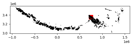
2) Crop vector data to spatial extent of raster data#
2) Crop vector data to spatial extent of raster data#
The above plot shows the coverage of the vector dataset, in black, relative to the extent of the raster dataset, in red. We use the geopandas .clip() method to subset the RGI object (se_asia_prj) to the footprint of the ITS_LIVe object (bbox_dc) object.
#Subset rgi to bounds
se_asia_subset = gpd.clip(se_asia_prj, bbox_dc)
se_asia_subset.head()
| rgi_id | o1region | o2region | glims_id | anlys_id | subm_id | src_date | cenlon | cenlat | utm_zone | ... | zmin_m | zmax_m | zmed_m | zmean_m | slope_deg | aspect_deg | aspect_sec | dem_source | lmax_m | geometry | |
|---|---|---|---|---|---|---|---|---|---|---|---|---|---|---|---|---|---|---|---|---|---|
| 16373 | RGI2000-v7.0-G-15-16374 | 15 | 15-03 | G095930E29817N | 930178 | 752 | 2005-09-08T00:00:00 | 95.929916 | 29.817003 | 46 | ... | 4985.7314 | 5274.0435 | 5142.7660 | 5148.8170 | 27.024134 | 139.048110 | 4 | COPDEM30 | 756 | POLYGON Z ((783110.719 3302487.481 0.000, 7831... |
| 16374 | RGI2000-v7.0-G-15-16375 | 15 | 15-03 | G095925E29818N | 930160 | 752 | 2005-09-08T00:00:00 | 95.925181 | 29.818399 | 46 | ... | 4856.2790 | 5054.9253 | 4929.5560 | 4933.6890 | 44.126980 | 211.518448 | 6 | COPDEM30 | 366 | POLYGON Z ((782511.360 3302381.154 0.000, 7825... |
| 16376 | RGI2000-v7.0-G-15-16377 | 15 | 15-03 | G095915E29820N | 930107 | 752 | 2005-09-08T00:00:00 | 95.914583 | 29.819510 | 46 | ... | 5072.8910 | 5150.6196 | 5108.5020 | 5111.7217 | 23.980000 | 219.341537 | 6 | COPDEM30 | 170 | POLYGON Z ((781619.822 3302305.074 0.000, 7816... |
| 16371 | RGI2000-v7.0-G-15-16372 | 15 | 15-03 | G095936E29819N | 930215 | 752 | 2005-09-08T00:00:00 | 95.935554 | 29.819123 | 46 | ... | 4838.7646 | 5194.8840 | 5001.5117 | 4992.3706 | 25.684517 | 128.737870 | 4 | COPDEM30 | 931 | POLYGON Z ((783420.055 3302493.804 0.000, 7834... |
| 15879 | RGI2000-v7.0-G-15-15880 | 15 | 15-03 | G095459E29807N | 928789 | 752 | 1999-07-29T00:00:00 | 95.459374 | 29.807181 | 46 | ... | 3802.1846 | 4155.1255 | 4000.2695 | 4000.4404 | 28.155806 | 116.148640 | 4 | COPDEM30 | 776 | POLYGON Z ((737667.211 3300277.169 0.000, 7377... |
5 rows × 29 columns
We can use the geopandas .explore() method to interactively look at the RGI7 outlines contained within the ITS_LIVE granule:
m = folium.Map(max_lat = 31,max_lon = 95, min_lat = 29, min_lon = 97,
location=[30.2, 95.5], zoom_start=8)
bbox_dc.explore(m=m, style_kwds = {'fillColor':'None', 'color':'red'},
legend_kwds = {'labels': ['ITS_LIVE granule footprint']})
se_asia_subset.explore(m=m)
folium.LayerControl().add_to(m)
m
/home/runner/micromamba/envs/itslive_tutorial_env/lib/python3.11/site-packages/folium/features.py:1102: UserWarning: GeoJsonTooltip is not configured to render for GeoJson GeometryCollection geometries. Please consider reworking these features: [{'rgi_id': 'RGI2000-v7.0-G-15-16433', 'o1region': '15', 'o2region': '15-03', 'glims_id': 'G095721E29941N', 'anlys_id': 929520, 'subm_id': 752, 'src_date': '2005-09-08T00:00:00', 'cenlon': 95.7211016152286, 'cenlat': 29.940902187781784, 'utm_zone': 46, 'area_km2': 0.340954350813452, 'primeclass': 0, 'conn_lvl': 0, 'surge_type': 0, 'term_type': 9, 'glac_name': None, 'is_rgi6': 0, 'termlon': 95.72222864596793, 'termlat': 29.937137080413784, 'zmin_m': 4657.792, 'zmax_m': 5049.5625, 'zmed_m': 4825.1104, 'zmean_m': 4839.4185, 'slope_deg': 23.704372, 'aspect_deg': 145.20973, 'aspect_sec': 4, 'dem_source': 'COPDEM30', 'lmax_m': 891}, {'rgi_id': 'RGI2000-v7.0-G-15-12194', 'o1region': '15', 'o2region': '15-03', 'glims_id': 'G095869E30315N', 'anlys_id': 929951, 'subm_id': 752, 'src_date': '2005-09-08T00:00:00', 'cenlon': 95.86889789565677, 'cenlat': 30.3147685, 'utm_zone': 46, 'area_km2': 8.797406997273084, 'primeclass': 0, 'conn_lvl': 0, 'surge_type': 0, 'term_type': 9, 'glac_name': None, 'is_rgi6': 0, 'termlon': 95.89518363763428, 'termlat': 30.307036248571297, 'zmin_m': 4642.1445, 'zmax_m': 5278.752, 'zmed_m': 5011.06, 'zmean_m': 4993.9243, 'slope_deg': 12.372513, 'aspect_deg': 81.418945, 'aspect_sec': 3, 'dem_source': 'COPDEM30', 'lmax_m': 4994}, {'rgi_id': 'RGI2000-v7.0-G-15-11941', 'o1region': '15', 'o2region': '15-03', 'glims_id': 'G095301E30377N', 'anlys_id': 928228, 'subm_id': 752, 'src_date': '2007-08-20T00:00:00', 'cenlon': 95.30071978915663, 'cenlat': 30.3770025, 'utm_zone': 46, 'area_km2': 0.267701958906151, 'primeclass': 0, 'conn_lvl': 0, 'surge_type': 0, 'term_type': 9, 'glac_name': None, 'is_rgi6': 0, 'termlon': 95.30345982475616, 'termlat': 30.380097687364806, 'zmin_m': 5475.784, 'zmax_m': 5977.979, 'zmed_m': 5750.727, 'zmean_m': 5759.621, 'slope_deg': 41.069595, 'aspect_deg': 350.3331518173218, 'aspect_sec': 1, 'dem_source': 'COPDEM30', 'lmax_m': 807}] to MultiPolygon for full functionality.
https://tools.ietf.org/html/rfc7946#page-9
warnings.warn(
While the above code correctly produces a plot, it also throws an warning. For a detailed example of trouble shooting and resolving this kind of warning, proceed to Section D, otherwise, skip ahead to Part 2.
3) Optional: Handle different geometry types when visualizing vector data#
3) Optional: Handle different geometry types#
It looks like we’re getting a warning on the explore() method that is interfering with the functionality that displays feature info when you hover over a feature. Let’s dig into it and see what’s going on. It looks like the issue is being caused by rows of the GeoDataFrame object that have a ‘GeometryCollection’ geometry type. First, I’m going to copy the warning into a cell below. The warning is already in the form of a list of dictionaries, which makes it nice to work with:
Here is the error message separated from the problem geometries:
/home/../python3.11/site-packages/folium/features.py:1102: UserWarning: GeoJsonTooltip is not configured to render for GeoJson GeometryCollection geometries. Please consider reworking these features: ..... to MultiPolygon for full functionality.
And below are the problem geometries identified in the error message saved as a list of dictionaries:
problem_geoms = [{'rgi_id': 'RGI2000-v7.0-G-15-16433', 'o1region': '15', 'o2region': '15-03', 'glims_id': 'G095721E29941N', 'anlys_id': 929520, 'subm_id': 752, 'src_date': '2005-09-08T00:00:00', 'cenlon': 95.7211016152286, 'cenlat': 29.940902187781784, 'utm_zone': 46, 'area_km2': 0.340954350813452, 'primeclass': 0, 'conn_lvl': 0, 'surge_type': 0, 'term_type': 9, 'glac_name': None, 'is_rgi6': 0, 'termlon': 95.72222864596793, 'termlat': 29.937137080413784, 'zmin_m': 4657.792, 'zmax_m': 5049.5625, 'zmed_m': 4825.1104, 'zmean_m': 4839.4185, 'slope_deg': 23.704372, 'aspect_deg': 145.20973, 'aspect_sec': 4, 'dem_source': 'COPDEM30', 'lmax_m': 891},
{'rgi_id': 'RGI2000-v7.0-G-15-12194', 'o1region': '15', 'o2region': '15-03', 'glims_id': 'G095869E30315N', 'anlys_id': 929951, 'subm_id': 752, 'src_date': '2005-09-08T00:00:00', 'cenlon': 95.86889789565677, 'cenlat': 30.3147685, 'utm_zone': 46, 'area_km2': 8.797406997273084, 'primeclass': 0, 'conn_lvl': 0, 'surge_type': 0, 'term_type': 9, 'glac_name': None, 'is_rgi6': 0, 'termlon': 95.89518363763428, 'termlat': 30.307036248571297, 'zmin_m': 4642.1445, 'zmax_m': 5278.752, 'zmed_m': 5011.06, 'zmean_m': 4993.9243, 'slope_deg': 12.372513, 'aspect_deg': 81.418945, 'aspect_sec': 3, 'dem_source': 'COPDEM30', 'lmax_m': 4994},
{'rgi_id': 'RGI2000-v7.0-G-15-11941', 'o1region': '15', 'o2region': '15-03', 'glims_id': 'G095301E30377N', 'anlys_id': 928228, 'subm_id': 752, 'src_date': '2007-08-20T00:00:00', 'cenlon': 95.30071978915663, 'cenlat': 30.3770025, 'utm_zone': 46, 'area_km2': 0.267701958906151, 'primeclass': 0, 'conn_lvl': 0, 'surge_type': 0, 'term_type': 9, 'glac_name': None, 'is_rgi6': 0, 'termlon': 95.30345982475616, 'termlat': 30.380097687364806, 'zmin_m': 5475.784, 'zmax_m': 5977.979, 'zmed_m': 5750.727, 'zmean_m': 5759.621, 'slope_deg': 41.069595, 'aspect_deg': 350.3331518173218, 'aspect_sec': 1, 'dem_source': 'COPDEM30', 'lmax_m': 807}]
First, convert the problem_geoms object from a list of dictionary objects to a pandas.DataFrame object:
problem_geoms_df = pd.DataFrame(data=problem_geoms)
Next, make a list of the IDs of the glaciers in this dataframe:
problem_geom_ids = problem_geoms_df['glims_id'].to_list()
problem_geom_ids
['G095721E29941N', 'G095869E30315N', 'G095301E30377N']
Make a geopandas.GeoDataFrame object that is just the above-identified outlines:
problem_geoms_gdf = se_asia_subset.loc[se_asia_subset['glims_id'].isin(problem_geom_ids)]
Check the geometry-type of these outlines and compare them to another outline from the se_asia_subset object that wasn’t flagged:
problem_geoms_gdf.loc[problem_geoms_gdf['glims_id'] == 'G095301E30377N'].geom_type
11940 GeometryCollection
dtype: object
se_asia_subset.loc[se_asia_subset['rgi_id'] == 'RGI2000-v7.0-G-15-11754'].geom_type
11753 Polygon
dtype: object
Now, the warning we saw above makes more sense. Most features in se_asia_subset have geom_type = Polygon but the flagged features have geom_type= GeometryCollection.
Let’s dig a bit more into these flagged geometries. To do this, use the geopandas method explode() to split multiple geometries into multiple single geometries.
first_flagged_feature = problem_geoms_gdf[problem_geoms_gdf.glims_id == 'G095301E30377N'].geometry.explode(index_parts=True)
Printing this object shows that it actually contains a polygon geometry and a linestring geometry:
first_flagged_feature
11940 0 POLYGON Z ((721543.154 3362894.920 0.000, 7215...
1 LINESTRING Z (721119.337 3362535.315 0.000, 72...
Name: geometry, dtype: geometry
Let’s look at the other two:
second_flagged_feature = problem_geoms_gdf[problem_geoms_gdf.glims_id == 'G095869E30315N'].geometry.explode(index_parts=True)
second_flagged_feature
12193 0 POLYGON Z ((774975.604 3356334.670 0.000, 7749...
1 LINESTRING Z (776713.643 3359150.691 0.000, 77...
Name: geometry, dtype: geometry
third_flagged_feature = problem_geoms_gdf[problem_geoms_gdf.glims_id == 'G095721E29941N'].geometry.explode(index_parts=True)
third_flagged_feature
16432 0 POLYGON Z ((762550.755 3315675.227 0.000, 7625...
1 LINESTRING Z (762974.041 3315372.040 0.000, 76...
Name: geometry, dtype: geometry
Check out some properties of the line geometry objects, such as length:
print(third_flagged_feature[1:].length.iloc[0])
print(second_flagged_feature[1:].length.iloc[0])
print(third_flagged_feature[1:].length.iloc[0])
0.07253059141477144
0.07953751551272183
0.07253059141477144
It looks like all of the linestring objects are very small, possibly artifacts, and don’t need to remain in the dataset. For simplicity, we can remove them from the original object. There are different ways to do this, but here’s one approach:
Identify and remove all features with the
GeometryCollectiongeom_type:
se_asia_subset_polygon = se_asia_subset[~se_asia_subset['geometry'].apply(lambda x : x.geom_type=='GeometryCollection' )]
Remove the line geometries from the
GeometryCollectionfeatures:
se_asia_subset_geom_collection = se_asia_subset[se_asia_subset['geometry'].astype(object).apply(
lambda x : x.geom_type=='GeometryCollection' )]
Make an object that is just the features where
geom_type= Polygon:
keep_polygons = se_asia_subset_geom_collection.explode(index_parts=True).loc[se_asia_subset_geom_collection.explode(index_parts=True).geom_type == 'Polygon']
Append the polygons to the
se_asia_subset_polygonsobject:
se_asia_polygons = pd.concat([se_asia_subset_polygon,keep_polygons])
As a sanity check, let’s make sure that we didn’t lose any glacier outline features during all of that:
len(se_asia_subset['rgi_id']) == len(se_asia_polygons)
True
Great, we know that we have the same number of glaciers that we started with.
Now, let’s try visualizing the outlines with explore() again and seeing if the hover tools work:
se_asia_polygons.explore()
We can use the above interactive map to select a glacier to look at in more detail below.
C. Join raster and vector data - single glacier#
1) Crop ITS_LIVE granule to a single glacier outline#
1) Crop ITS_LIVE granule to a single glacier outline#
If we want to dig in and analyze this velocity dataset at smaller spatial scales, we first need to subset it. The following section and the next notebook (Single Glacier Data Analysis) will focus on the spatial scale of a single glacier.
#Select a glacier to subset to
single_glacier_vec = se_asia_subset.loc[se_asia_subset['rgi_id'] == 'RGI2000-v7.0-G-15-16257']
single_glacier_vec
| rgi_id | o1region | o2region | glims_id | anlys_id | subm_id | src_date | cenlon | cenlat | utm_zone | ... | zmin_m | zmax_m | zmed_m | zmean_m | slope_deg | aspect_deg | aspect_sec | dem_source | lmax_m | geometry | |
|---|---|---|---|---|---|---|---|---|---|---|---|---|---|---|---|---|---|---|---|---|---|
| 16256 | RGI2000-v7.0-G-15-16257 | 15 | 15-03 | G095962E29920N | 930314 | 752 | 2005-09-08T00:00:00 | 95.961972 | 29.920094 | 46 | ... | 4320.7065 | 5937.84 | 5179.605 | 5131.8877 | 22.803406 | 100.811325 | 3 | COPDEM30 | 5958 | POLYGON Z ((788176.951 3315860.842 0.000, 7882... |
1 rows × 29 columns
#Write it to file to that it can be used later
single_glacier_vec.to_file('../data/single_glacier_vec.json', driver='GeoJSON')
Check to see if the ITS_LIVE raster dataset has an assigned CRS attribute. We already know that the data is projected in the correct coordinate reference system (CRS), but the object may not be ‘CRS-aware’ yet (ie. have an attribute specifying its CRS). This is necessary for spatial operations such as clipping and reprojection. If dc_rechunk doesn’t have a CRS attribute, use rio.write_crs() to assign it. For more detail, see Rioxarray’s CRS Management documentation.
dc_rechunk.rio.crs
It doesn’t have a CRS attribute, so we assign it:
dc_rechunk = dc_rechunk.rio.write_crs(f"epsg:{dc_rechunk.attrs['projection']}", inplace=True)
dc_rechunk.rio.crs
CRS.from_epsg(32646)
Now, use the subset vector data object and Rioxarray’s .clip() method to crop the data cube.
%%time
single_glacier_raster = dc_rechunk.rio.clip(single_glacier_vec.geometry, single_glacier_vec.crs)
CPU times: user 752 ms, sys: 16.9 ms, total: 769 ms
Wall time: 767 ms
2) Write clipped object to file#
2) Write clipped object to file.#
We want to use single_glacier_raster in the following notebook without going through all of the steps of creating it again. So, we write the object to file as a Zarr data cube so that we can easily read it into memory when we need it next. However, we’ll see that there are a few steps we must go through before we can successfully write this object.
We first re-chunk the single_glacier_raster into more optimal chunk sizes:
single_glacier_raster = single_glacier_raster.chunk({'mid_date':20000,
'x':10,
'y':10})
At this point, if we tried to write single_glacier_raster (eg. single_glacier_raster.to_zarr('data/glacier_itslive.zarr', mode='w')), we would get two errors that are cause by the ways that attribute and encoding information are stored.
The first error is:
‘’‘ValueError: failed to prevent overwriting existing key grid_mapping in attrs. This is probably an encoding field used by xarray to describe how a variable is serialized. To proceed, remove this key from the variable’s attributes manually.
‘’’
This indicates that the ‘grid_mapping’ attribute of several variables (grid_mapping specifies that spatial reference information about the data can be found in the mapping coordinate variable) is prohibiting the object being written to file. Because I’ve checked to ensure that these attribute keys all have the expected value (eg: print([single_glacier_raster[var].attrs['grid_mapping'] for var in single_glacier_raster.data_vars if 'grid_mapping' in single_glacier_raster[var].attrs])), I can go ahead and delete this attribute to proceed with the write operation.
for var in single_glacier_raster.data_vars:
if 'grid_mapping' in single_glacier_raster[var].attrs:
del single_glacier_raster[var].attrs['grid_mapping']
Great, we’ve resolved one error, but as the next code cell will show, we would still run into an encoding error trying to write this object:
single_glacier_raster.to_zarr('../data/single_glacier_itslive.zarr', mode='w')
ValueError: Specified zarr chunks encoding['chunks']=(56147,) for variable named 'acquisition_date_img2' would overlap multiple dask chunks ((20000, 20000, 7892),) on the region (slice(None, None, None),). Writing this array in parallel with dask could lead to corrupted data. Consider either rechunking using `chunk()`, deleting or modifying `encoding['chunks']`, or specify `safe_chunks=False`.
This one relates back to the Zarr encodings that we examined at the beginning of this notebook. Remember that we saw variables that only exist along the mid_date dimension had .encoding['chunks'] = 56147 even though the length of the mid_date dimension is 47,892. This occurs because Xarray does not overwrite or drop encodings when an object is rechunked or otherwise modified. In these cases, we should manually update or delete the out-of-date encoding. You can read more discussion on this topic here. We can fix it in a similar way, deleting a key from the object’s encoding instead of attrs.
for var in single_glacier_raster.data_vars:
del single_glacier_raster[var].encoding['chunks']
Now, let’s try to write the object as a Zarr group.
single_glacier_raster.to_zarr('../data/single_glacier_itslive.zarr', mode='w')
<xarray.backends.zarr.ZarrStore at 0x7f9e331f1f40>
Conclusion
In this notebook, we read a large object into memory, re-organized it and clipped it to the footprint of a single area of interest. We then saved that object to disk so that it can be easily re-used. The next notebook demonstrates exploratory data analysis steps using the object we just wrote to disk.