1. Accessing cloud-hosted ITS_LIVE data
Introduction
This notebook demonstrates how to query and access cloud-hosted Inter-mission Time Series of Land Ice Velocity and Elevation (ITS_LIVE) data from Amazon Web Services (AWS) S3 buckets. These data are stored as Zarr data cubes, a cloud-optimized format for array data. They are read into memory as Xarray Datasets.
Note
This tutorial was updated Jan 2025 to reflect changes to ITS_LIVE data urls and various software libraries
Outline
A. Read ITS_LIVE data from AWS S3 using Xarray
Overview of ITS_LIVE data storage and catalog
Read ITS_LIVE data from S3 storage into memory
Check spatial footprint of data
Find ITS_LIVE granule for a point of interest
Read + visualize spatial footprint of ITS_LIVE data
Note, this should maybe become its own notebook and/or chapter
Learning goals
Concepts
Query and access cloud-optimized dataset from cloud object storage
Create a vector data object representing the footprint of a raster dataset
Preliminary visualization of data extent
Techniques
Use Xarray to open Zarr datacube stored in AWS S3 bucket
Interactive data visualization with hvplot
Create Geopandas
geodataframefrom Xarrayxr.Datasetobject
Expand the next cell to see specific packages used in this notebook and relevant system and version information.
Show code cell source Hide code cell source
%xmode minimal

import geopandas as gpd
import hvplot.pandas
import s3fs
from typing import Union
from shapely.geometry import Point, Polygon
import xarray as xr
Exception reporting mode: Minimal
A. Read ITS_LIVE data from AWS S3 using Xarray#
1) Overview of ITS_LIVE data storage and catalog#
The ITS_LIVE project details a number of data access options on their website. Here, we will be accessing ITS_LIVE data in the form of zarr data cubes that are stored in s3 buckets hosted by Amazon Web Services (AWS).
Let’s begin by looking at the GeoJSON data cubes catalog. Click this link to download the file. This catalog contains spatial information and properties of ITS_LIVE data cubes as well as the URL used to access each cube. Let’s take a look at the entry for a single data cube and the information that it contains:
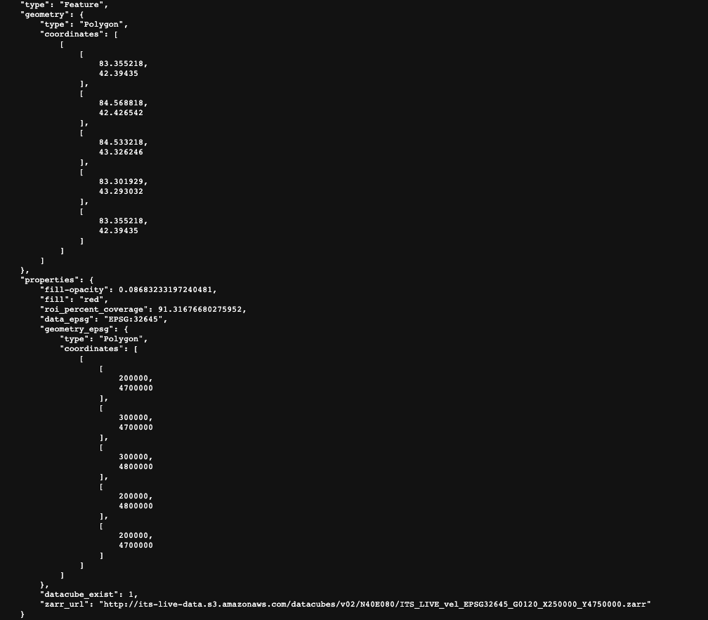
The top portion of the picture shows the spatial extent of the data cube in lat/lon units. Below that, we have properties such as the epsg code of the coordinate reference system, the spatial footprint in projected units and the url of the zarr object.
Let’s take a look at the url more in-depth:

From this link we can see that we are looking at its_live data located in an s3 bucket hosted by amazon AWS. We cans see that we’re looking in the data cube directory and what seems to be version 2. The next bit gives us information about the global location of the cube (N40E080). The actual file name ITS_LIVE_vel_EPSG32645_G0120_X250000_Y4750000.zarr tells us that we are looking at ice velocity data (its_live also has elevation data), in the CRS associated with EPSG 32645 (this code indicates UTM zone 45N). X250000_Y4750000 tells us more about the spatial footprint of the datacube within the UTM zone.
2) Read ITS_LIVE data from S3 storage into memory#
We’ve found the url associated with the tile we want to access, let’s try to open the data cube using Xarray.open_dataset():
url = 'http://its-live-data.s3.amazonaws.com/datacubes/v2/N30E090/ITS_LIVE_vel_EPSG32646_G0120_X750000_Y3350000.zarr'
In addition to passing url to xr.open_dataset(), we include chunks='auto'. This introduces dask into our workflow; chunks='auto' will choose chunk sizes that match the underlying data structure; this is often ideal, but sometimes you may need to specify different chunking schemes. You can read more about choosing good chunk sizes here; subsequent notebooks in this tutorial will explore different approaches to dask chunking.
dc = xr.open_dataset(url, decode_timedelta=True)
syntax error, unexpected WORD_WORD, expecting SCAN_ATTR or SCAN_DATASET or SCAN_ERROR
context: <?xml^ version="1.0" encoding="UTF-8"?><Error><Code>PermanentRedirect</Code><Message>The bucket you are attempting to access must be addressed using the specified endpoint. Please send all future requests to this endpoint.</Message><Endpoint>its-live-data.s3-us-west-2.amazonaws.com</Endpoint><Bucket>its-live-data</Bucket><RequestId>4HK62KBQ4G8PSQ19</RequestId><HostId>LWVOX3GLVAh5U47Zgww1YyjDbweZ0yttI1WsU3rGhAkNv8nnB/zfTqGY9gRdOY8fr0gBRlGWC/4=</HostId></Error>
KeyError: [<class 'netCDF4._netCDF4.Dataset'>, ('http://its-live-data.s3.amazonaws.com/datacubes/v2/N30E090/ITS_LIVE_vel_EPSG32646_G0120_X750000_Y3350000.zarr',), 'r', (('clobber', True), ('diskless', False), ('format', 'NETCDF4'), ('persist', False)), 'f9076f5d-9102-4a73-9e43-2aaface595c2']


During handling of the above exception, another exception occurred:

OSError: [Errno -72] NetCDF: Malformed or inaccessible DAP2 DDS or DAP4 DMR response: 'http://its-live-data.s3.amazonaws.com/datacubes/v2/N30E090/ITS_LIVE_vel_EPSG32646_G0120_X750000_Y3350000.zarr'
As you can see, this doesn’t quite work. When passing the url to xr.open_dataset(), if a backend isn’t specified, xarray will expect a netcdf file. Because we’re trying to open a zarr file we need to add an additional argument to xr.open_dataset(), shown in the next code cell. You can find more information here.
In the following cell, the argument chunks="auto" is passed, which introduces Dask into our workflow; chunks='auto' will choose chunk sizes that match the underlying data structure (this is generally ideal). You can read more about choosing good chunk sizes here; subsequent notebooks in this tutorial will explore different approaches to dask chunking.
dc = xr.open_dataset(url, engine= 'zarr', chunks="auto", decode_timedelta=True)
                                   # storage_options = {'anon':True}) <-- as of Fall 2023 this no longer needed
dc
<xarray.Dataset> Size: 771GB
Dimensions:                     (mid_date: 25243, y: 833, x: 833)
Coordinates:
  * mid_date                    (mid_date) datetime64[ns] 202kB 2022-06-07T04...
  * x                           (x) float64 7kB 7.001e+05 7.003e+05 ... 8e+05
  * y                           (y) float64 7kB 3.4e+06 3.4e+06 ... 3.3e+06
Data variables: (12/60)
    M11                         (mid_date, y, x) float32 70GB dask.array<chunksize=(25243, 30, 30), meta=np.ndarray>
    M11_dr_to_vr_factor         (mid_date) float32 101kB dask.array<chunksize=(25243,), meta=np.ndarray>
    M12                         (mid_date, y, x) float32 70GB dask.array<chunksize=(25243, 30, 30), meta=np.ndarray>
    M12_dr_to_vr_factor         (mid_date) float32 101kB dask.array<chunksize=(25243,), meta=np.ndarray>
    acquisition_date_img1       (mid_date) datetime64[ns] 202kB dask.array<chunksize=(25243,), meta=np.ndarray>
    acquisition_date_img2       (mid_date) datetime64[ns] 202kB dask.array<chunksize=(25243,), meta=np.ndarray>
    ...                          ...
    vy_error_modeled            (mid_date) float32 101kB dask.array<chunksize=(25243,), meta=np.ndarray>
    vy_error_slow               (mid_date) float32 101kB dask.array<chunksize=(25243,), meta=np.ndarray>
    vy_error_stationary         (mid_date) float32 101kB dask.array<chunksize=(25243,), meta=np.ndarray>
    vy_stable_shift             (mid_date) float32 101kB dask.array<chunksize=(25243,), meta=np.ndarray>
    vy_stable_shift_slow        (mid_date) float32 101kB dask.array<chunksize=(25243,), meta=np.ndarray>
    vy_stable_shift_stationary  (mid_date) float32 101kB dask.array<chunksize=(25243,), meta=np.ndarray>
Attributes: (12/19)
    Conventions:                CF-1.8
    GDAL_AREA_OR_POINT:         Area
    author:                     ITS_LIVE, a NASA MEaSUREs project (its-live.j...
    autoRIFT_parameter_file:    http://its-live-data.s3.amazonaws.com/autorif...
    datacube_software_version:  1.0
    date_created:               25-Sep-2023 22:00:23
    ...                         ...
    s3:                         s3://its-live-data/datacubes/v2/N30E090/ITS_L...
    skipped_granules:           s3://its-live-data/datacubes/v2/N30E090/ITS_L...
    time_standard_img1:         UTC
    time_standard_img2:         UTC
    title:                      ITS_LIVE datacube of image pair velocities
url: https://its-live-data.s3.amazonaws.com/datacu...- mid_date: 25243
- y: 833
- x: 833
- mid_date(mid_date)datetime64[ns]2022-06-07T04:21:44.211208960 .....
- description :
- midpoint of image 1 and image 2 acquisition date and time with granule's centroid longitude and latitude as microseconds
- standard_name :
- image_pair_center_date_with_time_separation
array(['2022-06-07T04:21:44.211208960', '2018-04-14T04:18:49.171219968', '2017-02-10T16:15:50.660901120', ..., '2013-05-20T04:08:31.155972096', '2015-10-17T04:11:05.527512064', '2015-11-10T04:11:15.457366016'], dtype='datetime64[ns]') - x(x)float647.001e+05 7.003e+05 ... 8e+05
- description :
- x coordinate of projection
- standard_name :
- projection_x_coordinate
array([700132.5, 700252.5, 700372.5, ..., 799732.5, 799852.5, 799972.5])
- y(y)float643.4e+06 3.4e+06 ... 3.3e+06 3.3e+06
- description :
- y coordinate of projection
- standard_name :
- projection_y_coordinate
array([3399907.5, 3399787.5, 3399667.5, ..., 3300307.5, 3300187.5, 3300067.5])
- M11(mid_date, y, x)float32dask.array<chunksize=(25243, 30, 30), meta=np.ndarray>
- description :
- conversion matrix element (1st row, 1st column) that can be multiplied with vx to give range pixel displacement dr (see Eq. A18 in https://www.mdpi.com/2072-4292/13/4/749)
- grid_mapping :
- mapping
- standard_name :
- conversion_matrix_element_11
- units :
- pixel/(meter/year)
Array Chunk Bytes 65.25 GiB 86.66 MiB Shape (25243, 833, 833) (25243, 30, 30) Dask graph 784 chunks in 2 graph layers Data type float32 numpy.ndarray - M11_dr_to_vr_factor(mid_date)float32dask.array<chunksize=(25243,), meta=np.ndarray>
- description :
- multiplicative factor that converts slant range pixel displacement dr to slant range velocity vr
- standard_name :
- M11_dr_to_vr_factor
- units :
- meter/(year*pixel)
Array Chunk Bytes 98.61 kiB 98.61 kiB Shape (25243,) (25243,) Dask graph 1 chunks in 2 graph layers Data type float32 numpy.ndarray - M12(mid_date, y, x)float32dask.array<chunksize=(25243, 30, 30), meta=np.ndarray>
- description :
- conversion matrix element (1st row, 2nd column) that can be multiplied with vy to give range pixel displacement dr (see Eq. A18 in https://www.mdpi.com/2072-4292/13/4/749)
- grid_mapping :
- mapping
- standard_name :
- conversion_matrix_element_12
- units :
- pixel/(meter/year)
Array Chunk Bytes 65.25 GiB 86.66 MiB Shape (25243, 833, 833) (25243, 30, 30) Dask graph 784 chunks in 2 graph layers Data type float32 numpy.ndarray - M12_dr_to_vr_factor(mid_date)float32dask.array<chunksize=(25243,), meta=np.ndarray>
- description :
- multiplicative factor that converts slant range pixel displacement dr to slant range velocity vr
- standard_name :
- M12_dr_to_vr_factor
- units :
- meter/(year*pixel)
Array Chunk Bytes 98.61 kiB 98.61 kiB Shape (25243,) (25243,) Dask graph 1 chunks in 2 graph layers Data type float32 numpy.ndarray - acquisition_date_img1(mid_date)datetime64[ns]dask.array<chunksize=(25243,), meta=np.ndarray>
- description :
- acquisition date and time of image 1
- standard_name :
- image1_acquition_date
Array Chunk Bytes 197.21 kiB 197.21 kiB Shape (25243,) (25243,) Dask graph 1 chunks in 2 graph layers Data type datetime64[ns] numpy.ndarray - acquisition_date_img2(mid_date)datetime64[ns]dask.array<chunksize=(25243,), meta=np.ndarray>
- description :
- acquisition date and time of image 2
- standard_name :
- image2_acquition_date
Array Chunk Bytes 197.21 kiB 197.21 kiB Shape (25243,) (25243,) Dask graph 1 chunks in 2 graph layers Data type datetime64[ns] numpy.ndarray - autoRIFT_software_version(mid_date)<U5dask.array<chunksize=(25243,), meta=np.ndarray>
- description :
- version of autoRIFT software
- standard_name :
- autoRIFT_software_version
Array Chunk Bytes 493.03 kiB 493.03 kiB Shape (25243,) (25243,) Dask graph 1 chunks in 2 graph layers Data type - chip_size_height(mid_date, y, x)float32dask.array<chunksize=(25243, 30, 30), meta=np.ndarray>
- chip_size_coordinates :
- Optical data: chip_size_coordinates = 'image projection geometry: width = x, height = y'. Radar data: chip_size_coordinates = 'radar geometry: width = range, height = azimuth'
- description :
- height of search template (chip)
- grid_mapping :
- mapping
- standard_name :
- chip_size_height
- units :
- m
- y_pixel_size :
- 10.0
Array Chunk Bytes 65.25 GiB 86.66 MiB Shape (25243, 833, 833) (25243, 30, 30) Dask graph 784 chunks in 2 graph layers Data type float32 numpy.ndarray - chip_size_width(mid_date, y, x)float32dask.array<chunksize=(25243, 30, 30), meta=np.ndarray>
- chip_size_coordinates :
- Optical data: chip_size_coordinates = 'image projection geometry: width = x, height = y'. Radar data: chip_size_coordinates = 'radar geometry: width = range, height = azimuth'
- description :
- width of search template (chip)
- grid_mapping :
- mapping
- standard_name :
- chip_size_width
- units :
- m
- x_pixel_size :
- 10.0
Array Chunk Bytes 65.25 GiB 86.66 MiB Shape (25243, 833, 833) (25243, 30, 30) Dask graph 784 chunks in 2 graph layers Data type float32 numpy.ndarray - date_center(mid_date)datetime64[ns]dask.array<chunksize=(25243,), meta=np.ndarray>
- description :
- midpoint of image 1 and image 2 acquisition date
- standard_name :
- image_pair_center_date
Array Chunk Bytes 197.21 kiB 197.21 kiB Shape (25243,) (25243,) Dask graph 1 chunks in 2 graph layers Data type datetime64[ns] numpy.ndarray - date_dt(mid_date)timedelta64[ns]dask.array<chunksize=(25243,), meta=np.ndarray>
- description :
- time separation between acquisition of image 1 and image 2
- standard_name :
- image_pair_time_separation
Array Chunk Bytes 197.21 kiB 197.21 kiB Shape (25243,) (25243,) Dask graph 1 chunks in 2 graph layers Data type timedelta64[ns] numpy.ndarray - floatingice(y, x)float32dask.array<chunksize=(833, 833), meta=np.ndarray>
- description :
- floating ice mask, 0 = non-floating-ice, 1 = floating-ice
- flag_meanings :
- non-ice ice
- flag_values :
- [0, 1]
- grid_mapping :
- mapping
- standard_name :
- floating ice mask
- url :
- https://its-live-data.s3.amazonaws.com/autorift_parameters/v001/N46_0120m_floatingice.tif
Array Chunk Bytes 2.65 MiB 2.65 MiB Shape (833, 833) (833, 833) Dask graph 1 chunks in 2 graph layers Data type float32 numpy.ndarray - granule_url(mid_date)<U1024dask.array<chunksize=(25243,), meta=np.ndarray>
- description :
- original granule URL
- standard_name :
- granule_url
Array Chunk Bytes 98.61 MiB 98.61 MiB Shape (25243,) (25243,) Dask graph 1 chunks in 2 graph layers Data type - interp_mask(mid_date, y, x)float32dask.array<chunksize=(25243, 30, 30), meta=np.ndarray>
- description :
- light interpolation mask
- flag_meanings :
- measured interpolated
- flag_values :
- [0, 1]
- grid_mapping :
- mapping
- standard_name :
- interpolated_value_mask
Array Chunk Bytes 65.25 GiB 86.66 MiB Shape (25243, 833, 833) (25243, 30, 30) Dask graph 784 chunks in 2 graph layers Data type float32 numpy.ndarray - landice(y, x)float32dask.array<chunksize=(833, 833), meta=np.ndarray>
- description :
- land ice mask, 0 = non-land-ice, 1 = land-ice
- flag_meanings :
- non-ice ice
- flag_values :
- [0, 1]
- grid_mapping :
- mapping
- standard_name :
- land ice mask
- url :
- https://its-live-data.s3.amazonaws.com/autorift_parameters/v001/N46_0120m_landice.tif
Array Chunk Bytes 2.65 MiB 2.65 MiB Shape (833, 833) (833, 833) Dask graph 1 chunks in 2 graph layers Data type float32 numpy.ndarray - mapping()<U1...
- GeoTransform :
- 700072.5 120.0 0 3399967.5 0 -120.0
- crs_wkt :
- PROJCS["WGS 84 / UTM zone 46N",GEOGCS["WGS 84",DATUM["WGS_1984",SPHEROID["WGS 84",6378137,298.257223563,AUTHORITY["EPSG","7030"]],AUTHORITY["EPSG","6326"]],PRIMEM["Greenwich",0,AUTHORITY["EPSG","8901"]],UNIT["degree",0.0174532925199433,AUTHORITY["EPSG","9122"]],AUTHORITY["EPSG","4326"]],PROJECTION["Transverse_Mercator"],PARAMETER["latitude_of_origin",0],PARAMETER["central_meridian",93],PARAMETER["scale_factor",0.9996],PARAMETER["false_easting",500000],PARAMETER["false_northing",0],UNIT["metre",1,AUTHORITY["EPSG","9001"]],AXIS["Easting",EAST],AXIS["Northing",NORTH],AUTHORITY["EPSG","32646"]]
- false_easting :
- 500000.0
- false_northing :
- 0.0
- grid_mapping_name :
- universal_transverse_mercator
- inverse_flattening :
- 298.257223563
- latitude_of_projection_origin :
- 0.0
- longitude_of_central_meridian :
- 93.0
- proj4text :
- +proj=utm +zone=46 +datum=WGS84 +units=m +no_defs
- scale_factor_at_central_meridian :
- 0.9996
- semi_major_axis :
- 6378137.0
- spatial_epsg :
- 32646
- spatial_ref :
- PROJCS["WGS 84 / UTM zone 46N",GEOGCS["WGS 84",DATUM["WGS_1984",SPHEROID["WGS 84",6378137,298.257223563,AUTHORITY["EPSG","7030"]],AUTHORITY["EPSG","6326"]],PRIMEM["Greenwich",0,AUTHORITY["EPSG","8901"]],UNIT["degree",0.0174532925199433,AUTHORITY["EPSG","9122"]],AUTHORITY["EPSG","4326"]],PROJECTION["Transverse_Mercator"],PARAMETER["latitude_of_origin",0],PARAMETER["central_meridian",93],PARAMETER["scale_factor",0.9996],PARAMETER["false_easting",500000],PARAMETER["false_northing",0],UNIT["metre",1,AUTHORITY["EPSG","9001"]],AXIS["Easting",EAST],AXIS["Northing",NORTH],AUTHORITY["EPSG","32646"]]
- utm_zone_number :
- 46.0
[1 values with dtype=<U1]
- mission_img1(mid_date)<U1dask.array<chunksize=(25243,), meta=np.ndarray>
- description :
- id of the mission that acquired image 1
- standard_name :
- image1_mission
Array Chunk Bytes 98.61 kiB 98.61 kiB Shape (25243,) (25243,) Dask graph 1 chunks in 2 graph layers Data type - mission_img2(mid_date)<U1dask.array<chunksize=(25243,), meta=np.ndarray>
- description :
- id of the mission that acquired image 2
- standard_name :
- image2_mission
Array Chunk Bytes 98.61 kiB 98.61 kiB Shape (25243,) (25243,) Dask graph 1 chunks in 2 graph layers Data type - roi_valid_percentage(mid_date)float32dask.array<chunksize=(25243,), meta=np.ndarray>
- description :
- percentage of pixels with a valid velocity estimate determined for the intersection of the full image pair footprint and the region of interest (roi) that defines where autoRIFT tried to estimate a velocity
- standard_name :
- region_of_interest_valid_pixel_percentage
Array Chunk Bytes 98.61 kiB 98.61 kiB Shape (25243,) (25243,) Dask graph 1 chunks in 2 graph layers Data type float32 numpy.ndarray - satellite_img1(mid_date)<U2dask.array<chunksize=(25243,), meta=np.ndarray>
- description :
- id of the satellite that acquired image 1
- standard_name :
- image1_satellite
Array Chunk Bytes 197.21 kiB 197.21 kiB Shape (25243,) (25243,) Dask graph 1 chunks in 2 graph layers Data type - satellite_img2(mid_date)<U2dask.array<chunksize=(25243,), meta=np.ndarray>
- description :
- id of the satellite that acquired image 2
- standard_name :
- image2_satellite
Array Chunk Bytes 197.21 kiB 197.21 kiB Shape (25243,) (25243,) Dask graph 1 chunks in 2 graph layers Data type - sensor_img1(mid_date)<U3dask.array<chunksize=(25243,), meta=np.ndarray>
- description :
- id of the sensor that acquired image 1
- standard_name :
- image1_sensor
Array Chunk Bytes 295.82 kiB 295.82 kiB Shape (25243,) (25243,) Dask graph 1 chunks in 2 graph layers Data type - sensor_img2(mid_date)<U3dask.array<chunksize=(25243,), meta=np.ndarray>
- description :
- id of the sensor that acquired image 2
- standard_name :
- image2_sensor
Array Chunk Bytes 295.82 kiB 295.82 kiB Shape (25243,) (25243,) Dask graph 1 chunks in 2 graph layers Data type - stable_count_slow(mid_date)uint16dask.array<chunksize=(25243,), meta=np.ndarray>
- description :
- number of valid pixels over slowest 25% of ice
- standard_name :
- stable_count_slow
- units :
- count
Array Chunk Bytes 49.30 kiB 49.30 kiB Shape (25243,) (25243,) Dask graph 1 chunks in 2 graph layers Data type uint16 numpy.ndarray - stable_count_stationary(mid_date)uint16dask.array<chunksize=(25243,), meta=np.ndarray>
- description :
- number of valid pixels over stationary or slow-flowing surfaces
- standard_name :
- stable_count_stationary
- units :
- count
Array Chunk Bytes 49.30 kiB 49.30 kiB Shape (25243,) (25243,) Dask graph 1 chunks in 2 graph layers Data type uint16 numpy.ndarray - stable_shift_flag(mid_date)uint8dask.array<chunksize=(25243,), meta=np.ndarray>
- description :
- flag for applying velocity bias correction: 0 = no correction; 1 = correction from overlapping stable surface mask (stationary or slow-flowing surfaces with velocity < 15 m/yr)(top priority); 2 = correction from slowest 25% of overlapping velocities (second priority)
- standard_name :
- stable_shift_flag
Array Chunk Bytes 24.65 kiB 24.65 kiB Shape (25243,) (25243,) Dask graph 1 chunks in 2 graph layers Data type uint8 numpy.ndarray - v(mid_date, y, x)float32dask.array<chunksize=(25243, 30, 30), meta=np.ndarray>
- description :
- velocity magnitude
- grid_mapping :
- mapping
- standard_name :
- land_ice_surface_velocity
- units :
- meter/year
Array Chunk Bytes 65.25 GiB 86.66 MiB Shape (25243, 833, 833) (25243, 30, 30) Dask graph 784 chunks in 2 graph layers Data type float32 numpy.ndarray - v_error(mid_date, y, x)float32dask.array<chunksize=(25243, 30, 30), meta=np.ndarray>
- description :
- velocity magnitude error
- grid_mapping :
- mapping
- standard_name :
- velocity_error
- units :
- meter/year
Array Chunk Bytes 65.25 GiB 86.66 MiB Shape (25243, 833, 833) (25243, 30, 30) Dask graph 784 chunks in 2 graph layers Data type float32 numpy.ndarray - va(mid_date, y, x)float32dask.array<chunksize=(25243, 30, 30), meta=np.ndarray>
- description :
- velocity in radar azimuth direction
- grid_mapping :
- mapping
Array Chunk Bytes 65.25 GiB 86.66 MiB Shape (25243, 833, 833) (25243, 30, 30) Dask graph 784 chunks in 2 graph layers Data type float32 numpy.ndarray - va_error(mid_date)float32dask.array<chunksize=(25243,), meta=np.ndarray>
- description :
- error for velocity in radar azimuth direction
- standard_name :
- va_error
- units :
- meter/year
Array Chunk Bytes 98.61 kiB 98.61 kiB Shape (25243,) (25243,) Dask graph 1 chunks in 2 graph layers Data type float32 numpy.ndarray - va_error_modeled(mid_date)float32dask.array<chunksize=(25243,), meta=np.ndarray>
- description :
- 1-sigma error calculated using a modeled error-dt relationship
- standard_name :
- va_error_modeled
- units :
- meter/year
Array Chunk Bytes 98.61 kiB 98.61 kiB Shape (25243,) (25243,) Dask graph 1 chunks in 2 graph layers Data type float32 numpy.ndarray - va_error_slow(mid_date)float32dask.array<chunksize=(25243,), meta=np.ndarray>
- description :
- RMSE over slowest 25% of retrieved velocities
- standard_name :
- va_error_slow
- units :
- meter/year
Array Chunk Bytes 98.61 kiB 98.61 kiB Shape (25243,) (25243,) Dask graph 1 chunks in 2 graph layers Data type float32 numpy.ndarray - va_error_stationary(mid_date)float32dask.array<chunksize=(25243,), meta=np.ndarray>
- description :
- RMSE over stable surfaces, stationary or slow-flowing surfaces with velocity < 15 m/yr identified from an external mask
- standard_name :
- va_error_stationary
- units :
- meter/year
Array Chunk Bytes 98.61 kiB 98.61 kiB Shape (25243,) (25243,) Dask graph 1 chunks in 2 graph layers Data type float32 numpy.ndarray - va_stable_shift(mid_date)float32dask.array<chunksize=(25243,), meta=np.ndarray>
- description :
- applied va shift calibrated using pixels over stable or slow surfaces
- standard_name :
- va_stable_shift
- units :
- meter/year
Array Chunk Bytes 98.61 kiB 98.61 kiB Shape (25243,) (25243,) Dask graph 1 chunks in 2 graph layers Data type float32 numpy.ndarray - va_stable_shift_slow(mid_date)float32dask.array<chunksize=(25243,), meta=np.ndarray>
- description :
- va shift calibrated using valid pixels over slowest 25% of retrieved velocities
- standard_name :
- va_stable_shift_slow
- units :
- meter/year
Array Chunk Bytes 98.61 kiB 98.61 kiB Shape (25243,) (25243,) Dask graph 1 chunks in 2 graph layers Data type float32 numpy.ndarray - va_stable_shift_stationary(mid_date)float32dask.array<chunksize=(25243,), meta=np.ndarray>
- description :
- va shift calibrated using valid pixels over stable surfaces, stationary or slow-flowing surfaces with velocity < 15 m/yr identified from an external mask
- standard_name :
- va_stable_shift_stationary
- units :
- meter/year
Array Chunk Bytes 98.61 kiB 98.61 kiB Shape (25243,) (25243,) Dask graph 1 chunks in 2 graph layers Data type float32 numpy.ndarray - vr(mid_date, y, x)float32dask.array<chunksize=(25243, 30, 30), meta=np.ndarray>
- description :
- velocity in radar range direction
- grid_mapping :
- mapping
Array Chunk Bytes 65.25 GiB 86.66 MiB Shape (25243, 833, 833) (25243, 30, 30) Dask graph 784 chunks in 2 graph layers Data type float32 numpy.ndarray - vr_error(mid_date)float32dask.array<chunksize=(25243,), meta=np.ndarray>
- description :
- error for velocity in radar range direction
- standard_name :
- vr_error
- units :
- meter/year
Array Chunk Bytes 98.61 kiB 98.61 kiB Shape (25243,) (25243,) Dask graph 1 chunks in 2 graph layers Data type float32 numpy.ndarray - vr_error_modeled(mid_date)float32dask.array<chunksize=(25243,), meta=np.ndarray>
- description :
- 1-sigma error calculated using a modeled error-dt relationship
- standard_name :
- vr_error_modeled
- units :
- meter/year
Array Chunk Bytes 98.61 kiB 98.61 kiB Shape (25243,) (25243,) Dask graph 1 chunks in 2 graph layers Data type float32 numpy.ndarray - vr_error_slow(mid_date)float32dask.array<chunksize=(25243,), meta=np.ndarray>
- description :
- RMSE over slowest 25% of retrieved velocities
- standard_name :
- vr_error_slow
- units :
- meter/year
Array Chunk Bytes 98.61 kiB 98.61 kiB Shape (25243,) (25243,) Dask graph 1 chunks in 2 graph layers Data type float32 numpy.ndarray - vr_error_stationary(mid_date)float32dask.array<chunksize=(25243,), meta=np.ndarray>
- description :
- RMSE over stable surfaces, stationary or slow-flowing surfaces with velocity < 15 m/yr identified from an external mask
- standard_name :
- vr_error_stationary
- units :
- meter/year
Array Chunk Bytes 98.61 kiB 98.61 kiB Shape (25243,) (25243,) Dask graph 1 chunks in 2 graph layers Data type float32 numpy.ndarray - vr_stable_shift(mid_date)float32dask.array<chunksize=(25243,), meta=np.ndarray>
- description :
- applied vr shift calibrated using pixels over stable or slow surfaces
- standard_name :
- vr_stable_shift
- units :
- meter/year
Array Chunk Bytes 98.61 kiB 98.61 kiB Shape (25243,) (25243,) Dask graph 1 chunks in 2 graph layers Data type float32 numpy.ndarray - vr_stable_shift_slow(mid_date)float32dask.array<chunksize=(25243,), meta=np.ndarray>
- description :
- vr shift calibrated using valid pixels over slowest 25% of retrieved velocities
- standard_name :
- vr_stable_shift_slow
- units :
- meter/year
Array Chunk Bytes 98.61 kiB 98.61 kiB Shape (25243,) (25243,) Dask graph 1 chunks in 2 graph layers Data type float32 numpy.ndarray - vr_stable_shift_stationary(mid_date)float32dask.array<chunksize=(25243,), meta=np.ndarray>
- description :
- vr shift calibrated using valid pixels over stable surfaces, stationary or slow-flowing surfaces with velocity < 15 m/yr identified from an external mask
- standard_name :
- vr_stable_shift_stationary
- units :
- meter/year
Array Chunk Bytes 98.61 kiB 98.61 kiB Shape (25243,) (25243,) Dask graph 1 chunks in 2 graph layers Data type float32 numpy.ndarray - vx(mid_date, y, x)float32dask.array<chunksize=(25243, 30, 30), meta=np.ndarray>
- description :
- velocity component in x direction
- grid_mapping :
- mapping
- standard_name :
- land_ice_surface_x_velocity
- units :
- meter/year
Array Chunk Bytes 65.25 GiB 86.66 MiB Shape (25243, 833, 833) (25243, 30, 30) Dask graph 784 chunks in 2 graph layers Data type float32 numpy.ndarray - vx_error(mid_date)float32dask.array<chunksize=(25243,), meta=np.ndarray>
- description :
- best estimate of x_velocity error: vx_error is populated according to the approach used for the velocity bias correction as indicated in "stable_shift_flag"
- standard_name :
- vx_error
- units :
- meter/year
Array Chunk Bytes 98.61 kiB 98.61 kiB Shape (25243,) (25243,) Dask graph 1 chunks in 2 graph layers Data type float32 numpy.ndarray - vx_error_modeled(mid_date)float32dask.array<chunksize=(25243,), meta=np.ndarray>
- description :
- 1-sigma error calculated using a modeled error-dt relationship
- standard_name :
- vx_error_modeled
- units :
- meter/year
Array Chunk Bytes 98.61 kiB 98.61 kiB Shape (25243,) (25243,) Dask graph 1 chunks in 2 graph layers Data type float32 numpy.ndarray - vx_error_slow(mid_date)float32dask.array<chunksize=(25243,), meta=np.ndarray>
- description :
- RMSE over slowest 25% of retrieved velocities
- standard_name :
- vx_error_slow
- units :
- meter/year
Array Chunk Bytes 98.61 kiB 98.61 kiB Shape (25243,) (25243,) Dask graph 1 chunks in 2 graph layers Data type float32 numpy.ndarray - vx_error_stationary(mid_date)float32dask.array<chunksize=(25243,), meta=np.ndarray>
- description :
- RMSE over stable surfaces, stationary or slow-flowing surfaces with velocity < 15 meter/year identified from an external mask
- standard_name :
- vx_error_stationary
- units :
- meter/year
Array Chunk Bytes 98.61 kiB 98.61 kiB Shape (25243,) (25243,) Dask graph 1 chunks in 2 graph layers Data type float32 numpy.ndarray - vx_stable_shift(mid_date)float32dask.array<chunksize=(25243,), meta=np.ndarray>
- description :
- applied vx shift calibrated using pixels over stable or slow surfaces
- standard_name :
- vx_stable_shift
- units :
- meter/year
Array Chunk Bytes 98.61 kiB 98.61 kiB Shape (25243,) (25243,) Dask graph 1 chunks in 2 graph layers Data type float32 numpy.ndarray - vx_stable_shift_slow(mid_date)float32dask.array<chunksize=(25243,), meta=np.ndarray>
- description :
- vx shift calibrated using valid pixels over slowest 25% of retrieved velocities
- standard_name :
- vx_stable_shift_slow
- units :
- meter/year
Array Chunk Bytes 98.61 kiB 98.61 kiB Shape (25243,) (25243,) Dask graph 1 chunks in 2 graph layers Data type float32 numpy.ndarray - vx_stable_shift_stationary(mid_date)float32dask.array<chunksize=(25243,), meta=np.ndarray>
- description :
- vx shift calibrated using valid pixels over stable surfaces, stationary or slow-flowing surfaces with velocity < 15 m/yr identified from an external mask
- standard_name :
- vx_stable_shift_stationary
- units :
- meter/year
Array Chunk Bytes 98.61 kiB 98.61 kiB Shape (25243,) (25243,) Dask graph 1 chunks in 2 graph layers Data type float32 numpy.ndarray - vy(mid_date, y, x)float32dask.array<chunksize=(25243, 30, 30), meta=np.ndarray>
- description :
- velocity component in y direction
- grid_mapping :
- mapping
- standard_name :
- land_ice_surface_y_velocity
- units :
- meter/year
Array Chunk Bytes 65.25 GiB 86.66 MiB Shape (25243, 833, 833) (25243, 30, 30) Dask graph 784 chunks in 2 graph layers Data type float32 numpy.ndarray - vy_error(mid_date)float32dask.array<chunksize=(25243,), meta=np.ndarray>
- description :
- best estimate of y_velocity error: vy_error is populated according to the approach used for the velocity bias correction as indicated in "stable_shift_flag"
- standard_name :
- vy_error
- units :
- meter/year
Array Chunk Bytes 98.61 kiB 98.61 kiB Shape (25243,) (25243,) Dask graph 1 chunks in 2 graph layers Data type float32 numpy.ndarray - vy_error_modeled(mid_date)float32dask.array<chunksize=(25243,), meta=np.ndarray>
- description :
- 1-sigma error calculated using a modeled error-dt relationship
- standard_name :
- vy_error_modeled
- units :
- meter/year
Array Chunk Bytes 98.61 kiB 98.61 kiB Shape (25243,) (25243,) Dask graph 1 chunks in 2 graph layers Data type float32 numpy.ndarray - vy_error_slow(mid_date)float32dask.array<chunksize=(25243,), meta=np.ndarray>
- description :
- RMSE over slowest 25% of retrieved velocities
- standard_name :
- vy_error_slow
- units :
- meter/year
Array Chunk Bytes 98.61 kiB 98.61 kiB Shape (25243,) (25243,) Dask graph 1 chunks in 2 graph layers Data type float32 numpy.ndarray - vy_error_stationary(mid_date)float32dask.array<chunksize=(25243,), meta=np.ndarray>
- description :
- RMSE over stable surfaces, stationary or slow-flowing surfaces with velocity < 15 meter/year identified from an external mask
- standard_name :
- vy_error_stationary
- units :
- meter/year
Array Chunk Bytes 98.61 kiB 98.61 kiB Shape (25243,) (25243,) Dask graph 1 chunks in 2 graph layers Data type float32 numpy.ndarray - vy_stable_shift(mid_date)float32dask.array<chunksize=(25243,), meta=np.ndarray>
- description :
- applied vy shift calibrated using pixels over stable or slow surfaces
- standard_name :
- vy_stable_shift
- units :
- meter/year
Array Chunk Bytes 98.61 kiB 98.61 kiB Shape (25243,) (25243,) Dask graph 1 chunks in 2 graph layers Data type float32 numpy.ndarray - vy_stable_shift_slow(mid_date)float32dask.array<chunksize=(25243,), meta=np.ndarray>
- description :
- vy shift calibrated using valid pixels over slowest 25% of retrieved velocities
- standard_name :
- vy_stable_shift_slow
- units :
- meter/year
Array Chunk Bytes 98.61 kiB 98.61 kiB Shape (25243,) (25243,) Dask graph 1 chunks in 2 graph layers Data type float32 numpy.ndarray - vy_stable_shift_stationary(mid_date)float32dask.array<chunksize=(25243,), meta=np.ndarray>
- description :
- vy shift calibrated using valid pixels over stable surfaces, stationary or slow-flowing surfaces with velocity < 15 m/yr identified from an external mask
- standard_name :
- vy_stable_shift_stationary
- units :
- meter/year
Array Chunk Bytes 98.61 kiB 98.61 kiB Shape (25243,) (25243,) Dask graph 1 chunks in 2 graph layers Data type float32 numpy.ndarray
- mid_datePandasIndex
PandasIndex(DatetimeIndex(['2022-06-07 04:21:44.211208960', '2018-04-14 04:18:49.171219968', '2017-02-10 16:15:50.660901120', '2022-04-03 04:19:01.211214080', '2021-07-22 04:16:46.210427904', '2019-03-15 04:15:44.180925952', '2002-09-15 03:59:12.379172096', '2002-12-28 03:42:16.181281024', '2021-06-29 16:16:10.210323968', '2022-03-26 16:18:35.211123968', ... '2015-03-15 04:10:27.667560960', '2012-11-25 04:08:32.642952960', '2012-12-27 04:08:58.362065920', '2017-05-27 04:10:08.145324032', '2016-12-06 04:11:32.294059776', '2013-04-18 04:08:52.932247040', '2017-05-07 04:11:30.865388288', '2013-05-20 04:08:31.155972096', '2015-10-17 04:11:05.527512064', '2015-11-10 04:11:15.457366016'], dtype='datetime64[ns]', name='mid_date', length=25243, freq=None)) - xPandasIndex
PandasIndex(Index([700132.5, 700252.5, 700372.5, 700492.5, 700612.5, 700732.5, 700852.5, 700972.5, 701092.5, 701212.5, ... 798892.5, 799012.5, 799132.5, 799252.5, 799372.5, 799492.5, 799612.5, 799732.5, 799852.5, 799972.5], dtype='float64', name='x', length=833)) - yPandasIndex
PandasIndex(Index([3399907.5, 3399787.5, 3399667.5, 3399547.5, 3399427.5, 3399307.5,
       3399187.5, 3399067.5, 3398947.5, 3398827.5,
       ...
       3301147.5, 3301027.5, 3300907.5, 3300787.5, 3300667.5, 3300547.5,
       3300427.5, 3300307.5, 3300187.5, 3300067.5],
      dtype='float64', name='y', length=833))
- Conventions :
- CF-1.8
- GDAL_AREA_OR_POINT :
- Area
- author :
- ITS_LIVE, a NASA MEaSUREs project (its-live.jpl.nasa.gov)
- autoRIFT_parameter_file :
- http://its-live-data.s3.amazonaws.com/autorift_parameters/v001/autorift_landice_0120m.shp
- datacube_software_version :
- 1.0
- date_created :
- 25-Sep-2023 22:00:23
- date_updated :
- 25-Sep-2023 22:00:23
- geo_polygon :
- [[95.06959008486952, 29.814255053135895], [95.32812062059084, 29.809951334550703], [95.58659184122865, 29.80514261876954], [95.84499718862224, 29.7998293459177], [96.10333011481168, 29.79401200205343], [96.11032804508507, 30.019297601073085], [96.11740568350054, 30.244573983323825], [96.12456379063154, 30.469841094022847], [96.1318031397002, 30.695098878594504], [95.87110827645229, 30.70112924501256], [95.61033817656023, 30.7066371044805], [95.34949964126946, 30.711621947056347], [95.08859948278467, 30.716083310981194], [95.08376623410525, 30.49063893600811], [95.07898726183609, 30.26518607254204], [95.0742620484426, 30.039724763743482], [95.06959008486952, 29.814255053135895]]
- institution :
- NASA Jet Propulsion Laboratory (JPL), California Institute of Technology
- latitude :
- 30.26
- longitude :
- 95.6
- proj_polygon :
- [[700000, 3300000], [725000.0, 3300000.0], [750000.0, 3300000.0], [775000.0, 3300000.0], [800000, 3300000], [800000.0, 3325000.0], [800000.0, 3350000.0], [800000.0, 3375000.0], [800000, 3400000], [775000.0, 3400000.0], [750000.0, 3400000.0], [725000.0, 3400000.0], [700000, 3400000], [700000.0, 3375000.0], [700000.0, 3350000.0], [700000.0, 3325000.0], [700000, 3300000]]
- projection :
- 32646
- s3 :
- s3://its-live-data/datacubes/v2/N30E090/ITS_LIVE_vel_EPSG32646_G0120_X750000_Y3350000.zarr
- skipped_granules :
- s3://its-live-data/datacubes/v2/N30E090/ITS_LIVE_vel_EPSG32646_G0120_X750000_Y3350000.json
- time_standard_img1 :
- UTC
- time_standard_img2 :
- UTC
- title :
- ITS_LIVE datacube of image pair velocities
- url :
- https://its-live-data.s3.amazonaws.com/datacubes/v2/N30E090/ITS_LIVE_vel_EPSG32646_G0120_X750000_Y3350000.zarr
This one worked! Let’s stop here and define a function that we can use to read additional s3 objects into memory as Xarray Datasets. This will come in handy later in this notebook and in subsequent notebooks.
def read_in_s3(http_url:str, chunks:Union[None, str, dict] = 'auto') -> xr.Dataset:
    """I'm a function that takes a url pointing to the location of a zarr data cube.
    I return an Xarray Dataset. I can take an optional chunk argument which specifies
    how the data will be chunked when read into memory"""

    #s3_url = http_url.replace('http','s3')   <-- as of Fall 2023, can pass http urls directly to xr.open_dataset()
    #s3_url = s3_url.replace('.s3.amazonaws.com','')

    datacube = xr.open_dataset(http_url, engine = 'zarr',
                                #storage_options={'anon':True},
                                chunks = chunks)

    return datacube
3) Check spatial footprint of data#
We just read in a very large dataset. We’d like an easy way to be able to visualize the footprint of this data to ensure we specified the correct location without plotting a data variable over the entire footprint, which would be much more computationally and time-intensive. The following function creates a GeoPandas.GeoDataFrame describing the spatial footprint of an xr.Dataset.
def get_bounds_polygon(input_xr: xr.Dataset) -> gpd.GeoDataFrame:
    """ I'm a function that takes an Xarray Dataset and returns a GeoPandas DataFrame of the bounding box of the Xarray Dataset."""

    xmin = input_xr.coords['x'].data.min()
    xmax = input_xr.coords['x'].data.max()

    ymin = input_xr.coords['y'].data.min()
    ymax = input_xr.coords['y'].data.max()

    pts_ls = [(xmin, ymin), (xmax, ymin),(xmax, ymax), (xmin, ymax), (xmin, ymin)]

    crs = f"epsg:{input_xr.mapping.spatial_epsg}"

    polygon_geom = Polygon(pts_ls)
    polygon = gpd.GeoDataFrame(index=[0], crs=crs, geometry=[polygon_geom])

    return polygon
Now let’s take a look at the cube we’ve already read:
bbox = get_bounds_polygon(dc)
get_bounds_polygon() returns a geopandas.GeoDataFrame object in the same projection as the velocity data object (local UTM). Re-project to latitude/longitude to view the object more easily on a map:
bbox = bbox.to_crs('EPSG:4326')
To visualize the footprint, we use the interactive plotting library, hvPlot.
poly = bbox.hvplot(legend=True,alpha=0.3, tiles='ESRI', color='red', geo=True)
poly
B. Query ITS_LIVE catalog#
1) Find ITS_LIVE granule for a point of interest#
Let’s look in a different region and see how we could search the ITS_LIVE data cube catalog for the granule that covers our location of interest. There are many ways to do this, this is just one example.
First, we read in the catalog geojson file:
itslive_catalog = gpd.read_file('https://its-live-data.s3.amazonaws.com/datacubes/catalog_v02.json')
Below is a function to query the catalog for the s3 url covering a given point. You could easily tweak this function (or write your own!) to select granules based on different properties. Play around with the itslive_catalog object to become more familiar with the data it contains and different options for indexing.
Note: since this tutorial was originally written, the ITS_LIVE Python Client was released. This is a great way to access ITS_LIVE data cubes.
fs  = s3fs.S3FileSystem(anon=True)
fs
<s3fs.core.S3FileSystem at 0x7fe871fd1e50>
def find_granule_by_point(input_point: list) -> str:
    """ I take a point in [lon, lat] format and return the url of the granule containing specified point.
    Point must be passed in EPSG:4326."""

    catalog = gpd.read_file('https://its-live-data.s3.amazonaws.com/datacubes/catalog_v02.json')

    #make shapely point of input point
    p = gpd.GeoSeries([Point(input_point[0], input_point[1])],crs='EPSG:4326')
    #make gdf of point
    gdf = gdf = gpd.GeoDataFrame({'label': 'point',
                                  'geometry':p})
    #find row of granule
    granule = catalog.sjoin(gdf, how='inner')

    url = granule['zarr_url'].values[0]
    return url
Choose a location in Alaska:
url = find_granule_by_point([-138.958776, 60.748561])
url
'http://its-live-data.s3.amazonaws.com/datacubes/v2-updated-october2024/N60W130/ITS_LIVE_vel_EPSG3413_G0120_X-3250000_Y250000.zarr'
Great, this function returned a single url corresponding to the data cube covering the point we supplied. Let’s use the read_in_s3 function we defined to open the datacube as an xarray.Dataset
datacube = read_in_s3(url)
2) Read + visualize spatial footprint of ITS_LIVE data#
Use the get_bounds_polyon function to take a look at the footprint using hvplot().
bbox_dc = get_bounds_polygon(datacube)
poly =  bbox_dc.to_crs('EPSG:4326').hvplot(legend=True,alpha=0.5, tiles='ESRI', color='red', geo=True)
poly
C. Overview of ITS_LIVE data#
Let’s briefly take a look at this ITS_LIVE time series object within the context of the Xarray data model. If you’re new to working with Xarray, the Data Structures documentation is very useful for getting a hang of the different components that are the building blocks of Xarray.Dataset objects.
datacube
<xarray.Dataset> Size: 4TB
Dimensions:                     (mid_date: 138421, y: 834, x: 834)
Coordinates:
  * mid_date                    (mid_date) datetime64[ns] 1MB 2020-03-16T08:4...
  * x                           (x) float64 7kB -3.3e+06 -3.3e+06 ... -3.2e+06
  * y                           (y) float64 7kB 2.999e+05 2.998e+05 ... 2e+05
Data variables: (12/60)
    M11                         (mid_date, y, x) float32 385GB dask.array<chunksize=(40000, 20, 20), meta=np.ndarray>
    M11_dr_to_vr_factor         (mid_date) float32 554kB dask.array<chunksize=(138421,), meta=np.ndarray>
    M12                         (mid_date, y, x) float32 385GB dask.array<chunksize=(40000, 20, 20), meta=np.ndarray>
    M12_dr_to_vr_factor         (mid_date) float32 554kB dask.array<chunksize=(138421,), meta=np.ndarray>
    acquisition_date_img1       (mid_date) datetime64[ns] 1MB dask.array<chunksize=(138421,), meta=np.ndarray>
    acquisition_date_img2       (mid_date) datetime64[ns] 1MB dask.array<chunksize=(138421,), meta=np.ndarray>
    ...                          ...
    vy_error_modeled            (mid_date) float32 554kB dask.array<chunksize=(138421,), meta=np.ndarray>
    vy_error_slow               (mid_date) float32 554kB dask.array<chunksize=(138421,), meta=np.ndarray>
    vy_error_stationary         (mid_date) float32 554kB dask.array<chunksize=(138421,), meta=np.ndarray>
    vy_stable_shift             (mid_date) float32 554kB dask.array<chunksize=(138421,), meta=np.ndarray>
    vy_stable_shift_slow        (mid_date) float32 554kB dask.array<chunksize=(138421,), meta=np.ndarray>
    vy_stable_shift_stationary  (mid_date) float32 554kB dask.array<chunksize=(138421,), meta=np.ndarray>
Attributes: (12/19)
    Conventions:                CF-1.8
    GDAL_AREA_OR_POINT:         Area
    author:                     ITS_LIVE, a NASA MEaSUREs project (its-live.j...
    autoRIFT_parameter_file:    http://its-live-data.s3.amazonaws.com/autorif...
    datacube_software_version:  1.0
    date_created:               25-Sep-2023 22:54:32
    ...                         ...
    s3:                         s3://its-live-data/datacubes/v2/N60W130/ITS_L...
    skipped_granules:           s3://its-live-data/datacubes/v2/N60W130/ITS_L...
    time_standard_img1:         UTC
    time_standard_img2:         UTC
    title:                      ITS_LIVE datacube of image pair velocities
url: https://its-live-data.s3.amazonaws.com/datacu...- mid_date: 138421
- y: 834
- x: 834
- mid_date(mid_date)datetime64[ns]2020-03-16T08:40:55.190909952 .....
- description :
- midpoint of image 1 and image 2 acquisition date and time with granule's centroid longitude and latitude as microseconds
- standard_name :
- image_pair_center_date_with_time_separation
array(['2020-03-16T08:40:55.190909952', '2018-11-07T08:40:25.180428032', '2015-05-06T03:03:14.440954112', ..., '2023-10-19T20:39:29.230416896', '2023-11-11T20:36:08.849937920', '2022-09-17T08:42:55.220417024'], dtype='datetime64[ns]') - x(x)float64-3.3e+06 -3.3e+06 ... -3.2e+06
- description :
- x coordinate of projection
- standard_name :
- projection_x_coordinate
array([-3299947.5, -3299827.5, -3299707.5, ..., -3200227.5, -3200107.5, -3199987.5]) - y(y)float642.999e+05 2.998e+05 ... 2e+05
- description :
- y coordinate of projection
- standard_name :
- projection_y_coordinate
array([299947.5, 299827.5, 299707.5, ..., 200227.5, 200107.5, 199987.5])
- M11(mid_date, y, x)float32dask.array<chunksize=(40000, 20, 20), meta=np.ndarray>
- description :
- conversion matrix element (1st row, 1st column) that can be multiplied with vx to give range pixel displacement dr (see Eq. A18 in https://www.mdpi.com/2072-4292/13/4/749)
- grid_mapping :
- mapping
- standard_name :
- conversion_matrix_element_11
- units :
- pixel/(meter/year)
Array Chunk Bytes 358.67 GiB 61.04 MiB Shape (138421, 834, 834) (40000, 20, 20) Dask graph 7056 chunks in 2 graph layers Data type float32 numpy.ndarray - M11_dr_to_vr_factor(mid_date)float32dask.array<chunksize=(138421,), meta=np.ndarray>
- description :
- multiplicative factor that converts slant range pixel displacement dr to slant range velocity vr
- standard_name :
- M11_dr_to_vr_factor
- units :
- meter/(year*pixel)
Array Chunk Bytes 540.71 kiB 540.71 kiB Shape (138421,) (138421,) Dask graph 1 chunks in 2 graph layers Data type float32 numpy.ndarray - M12(mid_date, y, x)float32dask.array<chunksize=(40000, 20, 20), meta=np.ndarray>
- description :
- conversion matrix element (1st row, 2nd column) that can be multiplied with vy to give range pixel displacement dr (see Eq. A18 in https://www.mdpi.com/2072-4292/13/4/749)
- grid_mapping :
- mapping
- standard_name :
- conversion_matrix_element_12
- units :
- pixel/(meter/year)
Array Chunk Bytes 358.67 GiB 61.04 MiB Shape (138421, 834, 834) (40000, 20, 20) Dask graph 7056 chunks in 2 graph layers Data type float32 numpy.ndarray - M12_dr_to_vr_factor(mid_date)float32dask.array<chunksize=(138421,), meta=np.ndarray>
- description :
- multiplicative factor that converts slant range pixel displacement dr to slant range velocity vr
- standard_name :
- M12_dr_to_vr_factor
- units :
- meter/(year*pixel)
Array Chunk Bytes 540.71 kiB 540.71 kiB Shape (138421,) (138421,) Dask graph 1 chunks in 2 graph layers Data type float32 numpy.ndarray - acquisition_date_img1(mid_date)datetime64[ns]dask.array<chunksize=(138421,), meta=np.ndarray>
- description :
- acquisition date and time of image 1
- standard_name :
- image1_acquition_date
Array Chunk Bytes 1.06 MiB 1.06 MiB Shape (138421,) (138421,) Dask graph 1 chunks in 2 graph layers Data type datetime64[ns] numpy.ndarray - acquisition_date_img2(mid_date)datetime64[ns]dask.array<chunksize=(138421,), meta=np.ndarray>
- description :
- acquisition date and time of image 2
- standard_name :
- image2_acquition_date
Array Chunk Bytes 1.06 MiB 1.06 MiB Shape (138421,) (138421,) Dask graph 1 chunks in 2 graph layers Data type datetime64[ns] numpy.ndarray - autoRIFT_software_version(mid_date)<U5dask.array<chunksize=(138421,), meta=np.ndarray>
- description :
- version of autoRIFT software
- standard_name :
- autoRIFT_software_version
Array Chunk Bytes 2.64 MiB 2.64 MiB Shape (138421,) (138421,) Dask graph 1 chunks in 2 graph layers Data type - chip_size_height(mid_date, y, x)float32dask.array<chunksize=(40000, 20, 20), meta=np.ndarray>
- chip_size_coordinates :
- Optical data: chip_size_coordinates = 'image projection geometry: width = x, height = y'. Radar data: chip_size_coordinates = 'radar geometry: width = range, height = azimuth'
- description :
- height of search template (chip)
- grid_mapping :
- mapping
- standard_name :
- chip_size_height
- units :
- m
- y_pixel_size :
- 10.0
Array Chunk Bytes 358.67 GiB 61.04 MiB Shape (138421, 834, 834) (40000, 20, 20) Dask graph 7056 chunks in 2 graph layers Data type float32 numpy.ndarray - chip_size_width(mid_date, y, x)float32dask.array<chunksize=(40000, 20, 20), meta=np.ndarray>
- chip_size_coordinates :
- Optical data: chip_size_coordinates = 'image projection geometry: width = x, height = y'. Radar data: chip_size_coordinates = 'radar geometry: width = range, height = azimuth'
- description :
- width of search template (chip)
- grid_mapping :
- mapping
- standard_name :
- chip_size_width
- units :
- m
- x_pixel_size :
- 10.0
Array Chunk Bytes 358.67 GiB 61.04 MiB Shape (138421, 834, 834) (40000, 20, 20) Dask graph 7056 chunks in 2 graph layers Data type float32 numpy.ndarray - date_center(mid_date)datetime64[ns]dask.array<chunksize=(138421,), meta=np.ndarray>
- description :
- midpoint of image 1 and image 2 acquisition date
- standard_name :
- image_pair_center_date
Array Chunk Bytes 1.06 MiB 1.06 MiB Shape (138421,) (138421,) Dask graph 1 chunks in 2 graph layers Data type datetime64[ns] numpy.ndarray - date_dt(mid_date)timedelta64[ns]dask.array<chunksize=(138421,), meta=np.ndarray>
- description :
- time separation between acquisition of image 1 and image 2
- standard_name :
- image_pair_time_separation
Array Chunk Bytes 1.06 MiB 1.06 MiB Shape (138421,) (138421,) Dask graph 1 chunks in 2 graph layers Data type timedelta64[ns] numpy.ndarray - floatingice(y, x)float32dask.array<chunksize=(834, 834), meta=np.ndarray>
- description :
- floating ice mask, 0 = non-floating-ice, 1 = floating-ice
- flag_meanings :
- non-ice ice
- flag_values :
- [0, 1]
- grid_mapping :
- mapping
- standard_name :
- floating ice mask
- url :
- https://its-live-data.s3.amazonaws.com/autorift_parameters/v001/NPS_0120m_floatingice.tif
Array Chunk Bytes 2.65 MiB 2.65 MiB Shape (834, 834) (834, 834) Dask graph 1 chunks in 2 graph layers Data type float32 numpy.ndarray - granule_url(mid_date)<U1024dask.array<chunksize=(32702,), meta=np.ndarray>
- description :
- original granule URL
- standard_name :
- granule_url
Array Chunk Bytes 540.71 MiB 127.74 MiB Shape (138421,) (32702,) Dask graph 5 chunks in 2 graph layers Data type - interp_mask(mid_date, y, x)float32dask.array<chunksize=(40000, 20, 20), meta=np.ndarray>
- description :
- light interpolation mask
- flag_meanings :
- measured interpolated
- flag_values :
- [0, 1]
- grid_mapping :
- mapping
- standard_name :
- interpolated_value_mask
Array Chunk Bytes 358.67 GiB 61.04 MiB Shape (138421, 834, 834) (40000, 20, 20) Dask graph 7056 chunks in 2 graph layers Data type float32 numpy.ndarray - landice(y, x)float32dask.array<chunksize=(834, 834), meta=np.ndarray>
- description :
- land ice mask, 0 = non-land-ice, 1 = land-ice
- flag_meanings :
- non-ice ice
- flag_values :
- [0, 1]
- grid_mapping :
- mapping
- standard_name :
- land ice mask
- url :
- https://its-live-data.s3.amazonaws.com/autorift_parameters/v001/NPS_0120m_landice.tif
Array Chunk Bytes 2.65 MiB 2.65 MiB Shape (834, 834) (834, 834) Dask graph 1 chunks in 2 graph layers Data type float32 numpy.ndarray - mapping()<U1...
- GeoTransform :
- -3300007.5 120.0 0 300007.5 0 -120.0
- crs_wkt :
- PROJCS["WGS 84 / NSIDC Sea Ice Polar Stereographic North",GEOGCS["WGS 84",DATUM["WGS_1984",SPHEROID["WGS 84",6378137,298.257223563,AUTHORITY["EPSG","7030"]],AUTHORITY["EPSG","6326"]],PRIMEM["Greenwich",0,AUTHORITY["EPSG","8901"]],UNIT["degree",0.0174532925199433,AUTHORITY["EPSG","9122"]],AUTHORITY["EPSG","4326"]],PROJECTION["Polar_Stereographic"],PARAMETER["latitude_of_origin",70],PARAMETER["central_meridian",-45],PARAMETER["false_easting",0],PARAMETER["false_northing",0],UNIT["metre",1,AUTHORITY["EPSG","9001"]],AXIS["Easting",SOUTH],AXIS["Northing",SOUTH],AUTHORITY["EPSG","3413"]]
- false_easting :
- 0.0
- false_northing :
- 0.0
- grid_mapping_name :
- polar_stereographic
- inverse_flattening :
- 298.257223563
- latitude_of_origin :
- 70.0
- latitude_of_projection_origin :
- 90.0
- proj4text :
- +proj=stere +lat_0=90 +lat_ts=70 +lon_0=-45 +x_0=0 +y_0=0 +datum=WGS84 +units=m +no_defs
- scale_factor_at_projection_origin :
- 1
- semi_major_axis :
- 6378137.0
- spatial_epsg :
- 3413
- spatial_ref :
- PROJCS["WGS 84 / NSIDC Sea Ice Polar Stereographic North",GEOGCS["WGS 84",DATUM["WGS_1984",SPHEROID["WGS 84",6378137,298.257223563,AUTHORITY["EPSG","7030"]],AUTHORITY["EPSG","6326"]],PRIMEM["Greenwich",0,AUTHORITY["EPSG","8901"]],UNIT["degree",0.0174532925199433,AUTHORITY["EPSG","9122"]],AUTHORITY["EPSG","4326"]],PROJECTION["Polar_Stereographic"],PARAMETER["latitude_of_origin",70],PARAMETER["central_meridian",-45],PARAMETER["false_easting",0],PARAMETER["false_northing",0],UNIT["metre",1,AUTHORITY["EPSG","9001"]],AXIS["Easting",SOUTH],AXIS["Northing",SOUTH],AUTHORITY["EPSG","3413"]]
- straight_vertical_longitude_from_pole :
- -45.0
[1 values with dtype=<U1]
- mission_img1(mid_date)<U1dask.array<chunksize=(138421,), meta=np.ndarray>
- description :
- id of the mission that acquired image 1
- standard_name :
- image1_mission
Array Chunk Bytes 540.71 kiB 540.71 kiB Shape (138421,) (138421,) Dask graph 1 chunks in 2 graph layers Data type - mission_img2(mid_date)<U1dask.array<chunksize=(138421,), meta=np.ndarray>
- description :
- id of the mission that acquired image 2
- standard_name :
- image2_mission
Array Chunk Bytes 540.71 kiB 540.71 kiB Shape (138421,) (138421,) Dask graph 1 chunks in 2 graph layers Data type - roi_valid_percentage(mid_date)float32dask.array<chunksize=(138421,), meta=np.ndarray>
- description :
- percentage of pixels with a valid velocity estimate determined for the intersection of the full image pair footprint and the region of interest (roi) that defines where autoRIFT tried to estimate a velocity
- standard_name :
- region_of_interest_valid_pixel_percentage
Array Chunk Bytes 540.71 kiB 540.71 kiB Shape (138421,) (138421,) Dask graph 1 chunks in 2 graph layers Data type float32 numpy.ndarray - satellite_img1(mid_date)<U2dask.array<chunksize=(138421,), meta=np.ndarray>
- description :
- id of the satellite that acquired image 1
- standard_name :
- image1_satellite
Array Chunk Bytes 1.06 MiB 1.06 MiB Shape (138421,) (138421,) Dask graph 1 chunks in 2 graph layers Data type - satellite_img2(mid_date)<U2dask.array<chunksize=(138421,), meta=np.ndarray>
- description :
- id of the satellite that acquired image 2
- standard_name :
- image2_satellite
Array Chunk Bytes 1.06 MiB 1.06 MiB Shape (138421,) (138421,) Dask graph 1 chunks in 2 graph layers Data type - sensor_img1(mid_date)<U3dask.array<chunksize=(138421,), meta=np.ndarray>
- description :
- id of the sensor that acquired image 1
- standard_name :
- image1_sensor
Array Chunk Bytes 1.58 MiB 1.58 MiB Shape (138421,) (138421,) Dask graph 1 chunks in 2 graph layers Data type - sensor_img2(mid_date)<U3dask.array<chunksize=(138421,), meta=np.ndarray>
- description :
- id of the sensor that acquired image 2
- standard_name :
- image2_sensor
Array Chunk Bytes 1.58 MiB 1.58 MiB Shape (138421,) (138421,) Dask graph 1 chunks in 2 graph layers Data type - stable_count_slow(mid_date)uint16dask.array<chunksize=(138421,), meta=np.ndarray>
- description :
- number of valid pixels over slowest 25% of ice
- standard_name :
- stable_count_slow
- units :
- count
Array Chunk Bytes 270.35 kiB 270.35 kiB Shape (138421,) (138421,) Dask graph 1 chunks in 2 graph layers Data type uint16 numpy.ndarray - stable_count_stationary(mid_date)uint16dask.array<chunksize=(138421,), meta=np.ndarray>
- description :
- number of valid pixels over stationary or slow-flowing surfaces
- standard_name :
- stable_count_stationary
- units :
- count
Array Chunk Bytes 270.35 kiB 270.35 kiB Shape (138421,) (138421,) Dask graph 1 chunks in 2 graph layers Data type uint16 numpy.ndarray - stable_shift_flag(mid_date)uint8dask.array<chunksize=(138421,), meta=np.ndarray>
- description :
- flag for applying velocity bias correction: 0 = no correction; 1 = correction from overlapping stable surface mask (stationary or slow-flowing surfaces with velocity < 15 m/yr)(top priority); 2 = correction from slowest 25% of overlapping velocities (second priority)
- standard_name :
- stable_shift_flag
Array Chunk Bytes 135.18 kiB 135.18 kiB Shape (138421,) (138421,) Dask graph 1 chunks in 2 graph layers Data type uint8 numpy.ndarray - v(mid_date, y, x)float32dask.array<chunksize=(40000, 20, 20), meta=np.ndarray>
- description :
- velocity magnitude
- grid_mapping :
- mapping
- standard_name :
- land_ice_surface_velocity
- units :
- meter/year
Array Chunk Bytes 358.67 GiB 61.04 MiB Shape (138421, 834, 834) (40000, 20, 20) Dask graph 7056 chunks in 2 graph layers Data type float32 numpy.ndarray - v_error(mid_date, y, x)float32dask.array<chunksize=(40000, 20, 20), meta=np.ndarray>
- description :
- velocity magnitude error
- grid_mapping :
- mapping
- standard_name :
- velocity_error
- units :
- meter/year
Array Chunk Bytes 358.67 GiB 61.04 MiB Shape (138421, 834, 834) (40000, 20, 20) Dask graph 7056 chunks in 2 graph layers Data type float32 numpy.ndarray - va(mid_date, y, x)float32dask.array<chunksize=(40000, 20, 20), meta=np.ndarray>
- description :
- velocity in radar azimuth direction
- grid_mapping :
- mapping
Array Chunk Bytes 358.67 GiB 61.04 MiB Shape (138421, 834, 834) (40000, 20, 20) Dask graph 7056 chunks in 2 graph layers Data type float32 numpy.ndarray - va_error(mid_date)float32dask.array<chunksize=(138421,), meta=np.ndarray>
- description :
- error for velocity in radar azimuth direction
- standard_name :
- va_error
- units :
- meter/year
Array Chunk Bytes 540.71 kiB 540.71 kiB Shape (138421,) (138421,) Dask graph 1 chunks in 2 graph layers Data type float32 numpy.ndarray - va_error_modeled(mid_date)float32dask.array<chunksize=(138421,), meta=np.ndarray>
- description :
- 1-sigma error calculated using a modeled error-dt relationship
- standard_name :
- va_error_modeled
- units :
- meter/year
Array Chunk Bytes 540.71 kiB 540.71 kiB Shape (138421,) (138421,) Dask graph 1 chunks in 2 graph layers Data type float32 numpy.ndarray - va_error_slow(mid_date)float32dask.array<chunksize=(138421,), meta=np.ndarray>
- description :
- RMSE over slowest 25% of retrieved velocities
- standard_name :
- va_error_slow
- units :
- meter/year
Array Chunk Bytes 540.71 kiB 540.71 kiB Shape (138421,) (138421,) Dask graph 1 chunks in 2 graph layers Data type float32 numpy.ndarray - va_error_stationary(mid_date)float32dask.array<chunksize=(138421,), meta=np.ndarray>
- description :
- RMSE over stable surfaces, stationary or slow-flowing surfaces with velocity < 15 m/yr identified from an external mask
- standard_name :
- va_error_stationary
- units :
- meter/year
Array Chunk Bytes 540.71 kiB 540.71 kiB Shape (138421,) (138421,) Dask graph 1 chunks in 2 graph layers Data type float32 numpy.ndarray - va_stable_shift(mid_date)float32dask.array<chunksize=(138421,), meta=np.ndarray>
- description :
- applied va shift calibrated using pixels over stable or slow surfaces
- standard_name :
- va_stable_shift
- units :
- meter/year
Array Chunk Bytes 540.71 kiB 540.71 kiB Shape (138421,) (138421,) Dask graph 1 chunks in 2 graph layers Data type float32 numpy.ndarray - va_stable_shift_slow(mid_date)float32dask.array<chunksize=(138421,), meta=np.ndarray>
- description :
- va shift calibrated using valid pixels over slowest 25% of retrieved velocities
- standard_name :
- va_stable_shift_slow
- units :
- meter/year
Array Chunk Bytes 540.71 kiB 540.71 kiB Shape (138421,) (138421,) Dask graph 1 chunks in 2 graph layers Data type float32 numpy.ndarray - va_stable_shift_stationary(mid_date)float32dask.array<chunksize=(138421,), meta=np.ndarray>
- description :
- va shift calibrated using valid pixels over stable surfaces, stationary or slow-flowing surfaces with velocity < 15 m/yr identified from an external mask
- standard_name :
- va_stable_shift_stationary
- units :
- meter/year
Array Chunk Bytes 540.71 kiB 540.71 kiB Shape (138421,) (138421,) Dask graph 1 chunks in 2 graph layers Data type float32 numpy.ndarray - vr(mid_date, y, x)float32dask.array<chunksize=(40000, 20, 20), meta=np.ndarray>
- description :
- velocity in radar range direction
- grid_mapping :
- mapping
Array Chunk Bytes 358.67 GiB 61.04 MiB Shape (138421, 834, 834) (40000, 20, 20) Dask graph 7056 chunks in 2 graph layers Data type float32 numpy.ndarray - vr_error(mid_date)float32dask.array<chunksize=(138421,), meta=np.ndarray>
- description :
- error for velocity in radar range direction
- standard_name :
- vr_error
- units :
- meter/year
Array Chunk Bytes 540.71 kiB 540.71 kiB Shape (138421,) (138421,) Dask graph 1 chunks in 2 graph layers Data type float32 numpy.ndarray - vr_error_modeled(mid_date)float32dask.array<chunksize=(138421,), meta=np.ndarray>
- description :
- 1-sigma error calculated using a modeled error-dt relationship
- standard_name :
- vr_error_modeled
- units :
- meter/year
Array Chunk Bytes 540.71 kiB 540.71 kiB Shape (138421,) (138421,) Dask graph 1 chunks in 2 graph layers Data type float32 numpy.ndarray - vr_error_slow(mid_date)float32dask.array<chunksize=(138421,), meta=np.ndarray>
- description :
- RMSE over slowest 25% of retrieved velocities
- standard_name :
- vr_error_slow
- units :
- meter/year
Array Chunk Bytes 540.71 kiB 540.71 kiB Shape (138421,) (138421,) Dask graph 1 chunks in 2 graph layers Data type float32 numpy.ndarray - vr_error_stationary(mid_date)float32dask.array<chunksize=(138421,), meta=np.ndarray>
- description :
- RMSE over stable surfaces, stationary or slow-flowing surfaces with velocity < 15 m/yr identified from an external mask
- standard_name :
- vr_error_stationary
- units :
- meter/year
Array Chunk Bytes 540.71 kiB 540.71 kiB Shape (138421,) (138421,) Dask graph 1 chunks in 2 graph layers Data type float32 numpy.ndarray - vr_stable_shift(mid_date)float32dask.array<chunksize=(138421,), meta=np.ndarray>
- description :
- applied vr shift calibrated using pixels over stable or slow surfaces
- standard_name :
- vr_stable_shift
- units :
- meter/year
Array Chunk Bytes 540.71 kiB 540.71 kiB Shape (138421,) (138421,) Dask graph 1 chunks in 2 graph layers Data type float32 numpy.ndarray - vr_stable_shift_slow(mid_date)float32dask.array<chunksize=(138421,), meta=np.ndarray>
- description :
- vr shift calibrated using valid pixels over slowest 25% of retrieved velocities
- standard_name :
- vr_stable_shift_slow
- units :
- meter/year
Array Chunk Bytes 540.71 kiB 540.71 kiB Shape (138421,) (138421,) Dask graph 1 chunks in 2 graph layers Data type float32 numpy.ndarray - vr_stable_shift_stationary(mid_date)float32dask.array<chunksize=(138421,), meta=np.ndarray>
- description :
- vr shift calibrated using valid pixels over stable surfaces, stationary or slow-flowing surfaces with velocity < 15 m/yr identified from an external mask
- standard_name :
- vr_stable_shift_stationary
- units :
- meter/year
Array Chunk Bytes 540.71 kiB 540.71 kiB Shape (138421,) (138421,) Dask graph 1 chunks in 2 graph layers Data type float32 numpy.ndarray - vx(mid_date, y, x)float32dask.array<chunksize=(40000, 20, 20), meta=np.ndarray>
- description :
- velocity component in x direction
- grid_mapping :
- mapping
- standard_name :
- land_ice_surface_x_velocity
- units :
- meter/year
Array Chunk Bytes 358.67 GiB 61.04 MiB Shape (138421, 834, 834) (40000, 20, 20) Dask graph 7056 chunks in 2 graph layers Data type float32 numpy.ndarray - vx_error(mid_date)float32dask.array<chunksize=(138421,), meta=np.ndarray>
- description :
- best estimate of x_velocity error: vx_error is populated according to the approach used for the velocity bias correction as indicated in "stable_shift_flag"
- standard_name :
- vx_error
- units :
- meter/year
Array Chunk Bytes 540.71 kiB 540.71 kiB Shape (138421,) (138421,) Dask graph 1 chunks in 2 graph layers Data type float32 numpy.ndarray - vx_error_modeled(mid_date)float32dask.array<chunksize=(138421,), meta=np.ndarray>
- description :
- 1-sigma error calculated using a modeled error-dt relationship
- standard_name :
- vx_error_modeled
- units :
- meter/year
Array Chunk Bytes 540.71 kiB 540.71 kiB Shape (138421,) (138421,) Dask graph 1 chunks in 2 graph layers Data type float32 numpy.ndarray - vx_error_slow(mid_date)float32dask.array<chunksize=(138421,), meta=np.ndarray>
- description :
- RMSE over slowest 25% of retrieved velocities
- standard_name :
- vx_error_slow
- units :
- meter/year
Array Chunk Bytes 540.71 kiB 540.71 kiB Shape (138421,) (138421,) Dask graph 1 chunks in 2 graph layers Data type float32 numpy.ndarray - vx_error_stationary(mid_date)float32dask.array<chunksize=(138421,), meta=np.ndarray>
- description :
- RMSE over stable surfaces, stationary or slow-flowing surfaces with velocity < 15 meter/year identified from an external mask
- standard_name :
- vx_error_stationary
- units :
- meter/year
Array Chunk Bytes 540.71 kiB 540.71 kiB Shape (138421,) (138421,) Dask graph 1 chunks in 2 graph layers Data type float32 numpy.ndarray - vx_stable_shift(mid_date)float32dask.array<chunksize=(138421,), meta=np.ndarray>
- description :
- applied vx shift calibrated using pixels over stable or slow surfaces
- standard_name :
- vx_stable_shift
- units :
- meter/year
Array Chunk Bytes 540.71 kiB 540.71 kiB Shape (138421,) (138421,) Dask graph 1 chunks in 2 graph layers Data type float32 numpy.ndarray - vx_stable_shift_slow(mid_date)float32dask.array<chunksize=(138421,), meta=np.ndarray>
- description :
- vx shift calibrated using valid pixels over slowest 25% of retrieved velocities
- standard_name :
- vx_stable_shift_slow
- units :
- meter/year
Array Chunk Bytes 540.71 kiB 540.71 kiB Shape (138421,) (138421,) Dask graph 1 chunks in 2 graph layers Data type float32 numpy.ndarray - vx_stable_shift_stationary(mid_date)float32dask.array<chunksize=(138421,), meta=np.ndarray>
- description :
- vx shift calibrated using valid pixels over stable surfaces, stationary or slow-flowing surfaces with velocity < 15 m/yr identified from an external mask
- standard_name :
- vx_stable_shift_stationary
- units :
- meter/year
Array Chunk Bytes 540.71 kiB 540.71 kiB Shape (138421,) (138421,) Dask graph 1 chunks in 2 graph layers Data type float32 numpy.ndarray - vy(mid_date, y, x)float32dask.array<chunksize=(40000, 20, 20), meta=np.ndarray>
- description :
- velocity component in y direction
- grid_mapping :
- mapping
- standard_name :
- land_ice_surface_y_velocity
- units :
- meter/year
Array Chunk Bytes 358.67 GiB 61.04 MiB Shape (138421, 834, 834) (40000, 20, 20) Dask graph 7056 chunks in 2 graph layers Data type float32 numpy.ndarray - vy_error(mid_date)float32dask.array<chunksize=(138421,), meta=np.ndarray>
- description :
- best estimate of y_velocity error: vy_error is populated according to the approach used for the velocity bias correction as indicated in "stable_shift_flag"
- standard_name :
- vy_error
- units :
- meter/year
Array Chunk Bytes 540.71 kiB 540.71 kiB Shape (138421,) (138421,) Dask graph 1 chunks in 2 graph layers Data type float32 numpy.ndarray - vy_error_modeled(mid_date)float32dask.array<chunksize=(138421,), meta=np.ndarray>
- description :
- 1-sigma error calculated using a modeled error-dt relationship
- standard_name :
- vy_error_modeled
- units :
- meter/year
Array Chunk Bytes 540.71 kiB 540.71 kiB Shape (138421,) (138421,) Dask graph 1 chunks in 2 graph layers Data type float32 numpy.ndarray - vy_error_slow(mid_date)float32dask.array<chunksize=(138421,), meta=np.ndarray>
- description :
- RMSE over slowest 25% of retrieved velocities
- standard_name :
- vy_error_slow
- units :
- meter/year
Array Chunk Bytes 540.71 kiB 540.71 kiB Shape (138421,) (138421,) Dask graph 1 chunks in 2 graph layers Data type float32 numpy.ndarray - vy_error_stationary(mid_date)float32dask.array<chunksize=(138421,), meta=np.ndarray>
- description :
- RMSE over stable surfaces, stationary or slow-flowing surfaces with velocity < 15 meter/year identified from an external mask
- standard_name :
- vy_error_stationary
- units :
- meter/year
Array Chunk Bytes 540.71 kiB 540.71 kiB Shape (138421,) (138421,) Dask graph 1 chunks in 2 graph layers Data type float32 numpy.ndarray - vy_stable_shift(mid_date)float32dask.array<chunksize=(138421,), meta=np.ndarray>
- description :
- applied vy shift calibrated using pixels over stable or slow surfaces
- standard_name :
- vy_stable_shift
- units :
- meter/year
Array Chunk Bytes 540.71 kiB 540.71 kiB Shape (138421,) (138421,) Dask graph 1 chunks in 2 graph layers Data type float32 numpy.ndarray - vy_stable_shift_slow(mid_date)float32dask.array<chunksize=(138421,), meta=np.ndarray>
- description :
- vy shift calibrated using valid pixels over slowest 25% of retrieved velocities
- standard_name :
- vy_stable_shift_slow
- units :
- meter/year
Array Chunk Bytes 540.71 kiB 540.71 kiB Shape (138421,) (138421,) Dask graph 1 chunks in 2 graph layers Data type float32 numpy.ndarray - vy_stable_shift_stationary(mid_date)float32dask.array<chunksize=(138421,), meta=np.ndarray>
- description :
- vy shift calibrated using valid pixels over stable surfaces, stationary or slow-flowing surfaces with velocity < 15 m/yr identified from an external mask
- standard_name :
- vy_stable_shift_stationary
- units :
- meter/year
Array Chunk Bytes 540.71 kiB 540.71 kiB Shape (138421,) (138421,) Dask graph 1 chunks in 2 graph layers Data type float32 numpy.ndarray
- mid_datePandasIndex
PandasIndex(DatetimeIndex(['2020-03-16 08:40:55.190909952', '2018-11-07 08:40:25.180428032', '2015-05-06 03:03:14.440954112', '2016-08-14 20:54:07.160510976', '2002-03-14 20:25:04.966016', '1999-12-04 20:23:49.902206976', '2021-09-27 20:53:36.210203904', '2021-12-18 20:40:26.210610944', '2020-06-26 08:32:50.200314624', '2011-07-02 08:22:51.810615040', ... '2023-03-18 20:41:44.220829952', '2023-09-14 20:42:16.230322944', '2023-07-06 20:45:19.221107968', '2024-01-15 08:40:25.230924032', '2023-10-23 20:30:38.377039872', '2024-03-05 08:43:30.240220928', '2023-08-30 08:33:30.230113792', '2023-10-19 20:39:29.230416896', '2023-11-11 20:36:08.849937920', '2022-09-17 08:42:55.220417024'], dtype='datetime64[ns]', name='mid_date', length=138421, freq=None)) - xPandasIndex
PandasIndex(Index([-3299947.5, -3299827.5, -3299707.5, -3299587.5, -3299467.5, -3299347.5, -3299227.5, -3299107.5, -3298987.5, -3298867.5, ... -3201067.5, -3200947.5, -3200827.5, -3200707.5, -3200587.5, -3200467.5, -3200347.5, -3200227.5, -3200107.5, -3199987.5], dtype='float64', name='x', length=834)) - yPandasIndex
PandasIndex(Index([299947.5, 299827.5, 299707.5, 299587.5, 299467.5, 299347.5, 299227.5,
       299107.5, 298987.5, 298867.5,
       ...
       201067.5, 200947.5, 200827.5, 200707.5, 200587.5, 200467.5, 200347.5,
       200227.5, 200107.5, 199987.5],
      dtype='float64', name='y', length=834))
- Conventions :
- CF-1.8
- GDAL_AREA_OR_POINT :
- Area
- author :
- ITS_LIVE, a NASA MEaSUREs project (its-live.jpl.nasa.gov)
- autoRIFT_parameter_file :
- http://its-live-data.s3.amazonaws.com/autorift_parameters/v001/autorift_landice_0120m.shp
- datacube_software_version :
- 1.0
- date_created :
- 25-Sep-2023 22:54:32
- date_updated :
- 13-Nov-2024 00:15:12
- geo_polygon :
- [[-138.46822925891712, 60.147756216807174], [-138.49463892725333, 60.36348555837142], [-138.52145337692224, 60.579416456816496], [-138.54868197390445, 60.79554754863715], [-138.57633437499737, 61.011877457917706], [-139.02199017702011, 60.9975093905528], [-139.46715906138928, 60.9814608009123], [-139.911788172506, 60.96373494822363], [-140.35582504285517, 60.944335424185965], [-140.31454566994478, 60.728589190850066], [-140.27389595735178, 60.513033250506986], [-140.23386164721643, 60.29766916958488], [-140.19442890773482, 60.082498496408085], [-139.7636416907262, 60.101242884393535], [-139.33231398318853, 60.11836944082792], [-138.90049374238188, 60.13387487895878], [-138.46822925891712, 60.147756216807174]]
- institution :
- NASA Jet Propulsion Laboratory (JPL), California Institute of Technology
- latitude :
- 60.55
- longitude :
- -139.4
- proj_polygon :
- [[-3300000, 200000], [-3275000.0, 200000.0], [-3250000.0, 200000.0], [-3225000.0, 200000.0], [-3200000, 200000], [-3200000.0, 225000.0], [-3200000.0, 250000.0], [-3200000.0, 275000.0], [-3200000, 300000], [-3225000.0, 300000.0], [-3250000.0, 300000.0], [-3275000.0, 300000.0], [-3300000, 300000], [-3300000.0, 275000.0], [-3300000.0, 250000.0], [-3300000.0, 225000.0], [-3300000, 200000]]
- projection :
- 3413
- s3 :
- s3://its-live-data/datacubes/v2/N60W130/ITS_LIVE_vel_EPSG3413_G0120_X-3250000_Y250000.zarr
- skipped_granules :
- s3://its-live-data/datacubes/v2/N60W130/ITS_LIVE_vel_EPSG3413_G0120_X-3250000_Y250000.json
- time_standard_img1 :
- UTC
- time_standard_img2 :
- UTC
- title :
- ITS_LIVE datacube of image pair velocities
- url :
- https://its-live-data.s3.amazonaws.com/datacubes/v2/N60W130/ITS_LIVE_vel_EPSG3413_G0120_X-3250000_Y250000.zarr
Data structure overview#
Dimensions + Coordinates#
This object has 3 dimensions,
mid_date,x, andy. Each dimension has a corresponding coordinate variable.If decide to add this section/content, should really move a lot of the Xarray variables to be coordinates, and/or least have a quick discussion of what many of the variables are and say that we will be focusing on these variables …
Data variables#
Expanding the ‘Data Variables’ label, you can see that there are many (60!) variables. Each variable exists along one or more dimension (eg.
(mid_date,x,y)), has an associated data type (eg.float32), and has an underlying array that holds that variable’s data.
Attributes#
Whereas data variables are by definition dimensional, there is usually a collection of scalar metadata that informs how data variables should be manipulated and interpreted. Scalar metadata is stored in attributes. All array-based Xarray objects (data variables, coordinate variables, DataArrays and Datasets) can have attributes attached to them.
Add section on CF conventions + metadata naming…#
Conclusion
This notebook demonstrated how to query and access a cloud-optimized remote sensing time series dataset stored in an AWS S3 bucket. The subsequent notebooks in this tutorial will go into much more detail on how to organize, examine and analyze this data.