3. Exploratory data analysis of a single glacier
Introduction
Overview
In the previous notebook, we walked through initial steps to read and organize a large raster dataset, and to understand it in the context of spatial areas of interest represented by vector data.
The previous notebook mainly focused on high-level processing operations:
reading a multi-dimensional dataset,
re-organizing along a given dimension,
reducing a large raster object to smaller areas of interest represented by vector data, and
strategies for completing these steps with larger-than-memory datasets.
In this notebook, we will continue performing initial data inspection and exploratory analysis but this time, focused on velocity data clipped to an individual glacier. We demonstrate Xarray functionality for common computations and visualizations.
Outline
Load raster data into memory and visualize with vector data
Examine data coverage
Break down by sensor
Combine sensor-specific subset
B. Examine velocity variability
Histograms and summary statistics
Spatial velocity variability
Temporal velocity variability
Temporal resampling
Grouped analysis by season
Learning goals
Concepts
Examining metadata, interpreting physical observable in the contxt of available metadata
Techniques
Using matplotlib to visualize raster and vector data with satellite imagery basemaps
Expand the next cell to see specific packages used in this notebook and relevant system and version information.
Show code cell source Hide code cell source
%xmode minimal
import contextily as cx
import geopandas as gpd
import matplotlib.pyplot as plt
import numpy as np
import rioxarray as rio
import scipy.stats
import warnings
import xarray as xr

warnings.simplefilter(action='ignore', category=FutureWarning)
Show code cell output Hide code cell output
Exception reporting mode: Minimal
A. Data exploration#
1) Load raster data into memory and visualize with vector data#
single_glacier_raster = xr.open_zarr('../data/single_glacier_itslive.zarr')
single_glacier_vector = gpd.read_file('../data/single_glacier_vec.json')
single_glacier_raster.nbytes/ 1e9
3.326255548
The above code cells show us that this dataset contains observations from Sentinel 1 & 2 and Landsat 4,5,6,7,8 & 9 satellite sensors. The dataset is 3.3 GB.
Next, we want to perform computations that require us to load this object into memory. To do this, we use the dask .compute() method, which turns a ‘lazy’ object into an in-memory object. If you try to run compute on too large of an object, your computer may run out of RAM and the kernel being used in this python session will die (if this happens, click ‘restart kernel’ from the kernel drop down menu above).
single_glacier_raster = single_glacier_raster.compute()
Now, if you expand the data object to look at the variables, you will see that they no long hold dask.array objects.
single_glacier_raster
<xarray.Dataset> Size: 3GB
Dimensions:                     (mid_date: 47892, y: 37, x: 40)
Coordinates:
  * mid_date                    (mid_date) datetime64[ns] 383kB 1986-09-11T03...
    spatial_ref                 int64 8B 0
  * x                           (x) float64 320B 7.843e+05 ... 7.889e+05
  * y                           (y) float64 296B 3.316e+06 ... 3.311e+06
Data variables: (12/60)
    M11                         (mid_date, y, x) float32 284MB nan nan ... nan
    M11_dr_to_vr_factor         (mid_date) float32 192kB nan nan nan ... nan nan
    M12                         (mid_date, y, x) float32 284MB nan nan ... nan
    M12_dr_to_vr_factor         (mid_date) float32 192kB nan nan nan ... nan nan
    acquisition_date_img1       (mid_date) datetime64[ns] 383kB 1986-07-25T03...
    acquisition_date_img2       (mid_date) datetime64[ns] 383kB 1986-10-29T03...
    ...                          ...
    vy_error_modeled            (mid_date) float32 192kB 97.0 64.6 ... 930.7
    vy_error_slow               (mid_date) float32 192kB 30.3 18.9 ... 61.7 50.1
    vy_error_stationary         (mid_date) float32 192kB 30.2 18.9 ... 61.6 50.1
    vy_stable_shift             (mid_date) float32 192kB 4.1 -6.9 ... 91.2 91.2
    vy_stable_shift_slow        (mid_date) float32 192kB 4.2 -6.9 ... 91.2 91.2
    vy_stable_shift_stationary  (mid_date) float32 192kB 4.1 -6.9 ... 91.2 91.2
Attributes: (12/19)
    Conventions:                CF-1.8
    GDAL_AREA_OR_POINT:         Area
    author:                     ITS_LIVE, a NASA MEaSUREs project (its-live.j...
    autoRIFT_parameter_file:    http://its-live-data.s3.amazonaws.com/autorif...
    datacube_software_version:  1.0
    date_created:               25-Sep-2023 22:00:23
    ...                         ...
    s3:                         s3://its-live-data/datacubes/v2/N30E090/ITS_L...
    skipped_granules:           s3://its-live-data/datacubes/v2/N30E090/ITS_L...
    time_standard_img1:         UTC
    time_standard_img2:         UTC
    title:                      ITS_LIVE datacube of image pair velocities
url: https://its-live-data.s3.amazonaws.com/datacu...- mid_date: 47892
- y: 37
- x: 40
- mid_date(mid_date)datetime64[ns]1986-09-11T03:31:15.003252992 .....
- description :
- midpoint of image 1 and image 2 acquisition date and time with granule's centroid longitude and latitude as microseconds
- standard_name :
- image_pair_center_date_with_time_separation
array(['1986-09-11T03:31:15.003252992', '1986-10-05T03:31:06.144750016', '1986-10-21T03:31:34.493249984', ..., '2024-10-29T04:18:09.241024000', '2024-10-29T04:18:09.241024000', '2024-10-29T04:18:09.241024000'], dtype='datetime64[ns]') - spatial_ref()int640
- GeoTransform :
- 784192.5 120.0 0.0 3315847.5 0.0 -120.0
array(0)
- x(x)float647.843e+05 7.844e+05 ... 7.889e+05
- axis :
- X
- description :
- x coordinate of projection
- long_name :
- x coordinate of projection
- standard_name :
- projection_x_coordinate
- units :
- metre
array([784252.5, 784372.5, 784492.5, 784612.5, 784732.5, 784852.5, 784972.5, 785092.5, 785212.5, 785332.5, 785452.5, 785572.5, 785692.5, 785812.5, 785932.5, 786052.5, 786172.5, 786292.5, 786412.5, 786532.5, 786652.5, 786772.5, 786892.5, 787012.5, 787132.5, 787252.5, 787372.5, 787492.5, 787612.5, 787732.5, 787852.5, 787972.5, 788092.5, 788212.5, 788332.5, 788452.5, 788572.5, 788692.5, 788812.5, 788932.5]) - y(y)float643.316e+06 3.316e+06 ... 3.311e+06
- axis :
- Y
- description :
- y coordinate of projection
- long_name :
- y coordinate of projection
- standard_name :
- projection_y_coordinate
- units :
- metre
array([3315787.5, 3315667.5, 3315547.5, 3315427.5, 3315307.5, 3315187.5,
       3315067.5, 3314947.5, 3314827.5, 3314707.5, 3314587.5, 3314467.5,
       3314347.5, 3314227.5, 3314107.5, 3313987.5, 3313867.5, 3313747.5,
       3313627.5, 3313507.5, 3313387.5, 3313267.5, 3313147.5, 3313027.5,
       3312907.5, 3312787.5, 3312667.5, 3312547.5, 3312427.5, 3312307.5,
       3312187.5, 3312067.5, 3311947.5, 3311827.5, 3311707.5, 3311587.5,
       3311467.5])
- M11(mid_date, y, x)float32nan nan nan nan ... nan nan nan nan
- description :
- conversion matrix element (1st row, 1st column) that can be multiplied with vx to give range pixel displacement dr (see Eq. A18 in https://www.mdpi.com/2072-4292/13/4/749)
- grid_mapping :
- mapping
- standard_name :
- conversion_matrix_element_11
- units :
- pixel/(meter/year)
array([[[nan, nan, nan, ..., nan, nan, nan], [nan, nan, nan, ..., nan, nan, nan], [nan, nan, nan, ..., nan, nan, nan], ..., [nan, nan, nan, ..., nan, nan, nan], [nan, nan, nan, ..., nan, nan, nan], [nan, nan, nan, ..., nan, nan, nan]], [[nan, nan, nan, ..., nan, nan, nan], [nan, nan, nan, ..., nan, nan, nan], [nan, nan, nan, ..., nan, nan, nan], ..., [nan, nan, nan, ..., nan, nan, nan], [nan, nan, nan, ..., nan, nan, nan], [nan, nan, nan, ..., nan, nan, nan]], [[nan, nan, nan, ..., nan, nan, nan], [nan, nan, nan, ..., nan, nan, nan], [nan, nan, nan, ..., nan, nan, nan], ..., ... ..., [nan, nan, nan, ..., nan, nan, nan], [nan, nan, nan, ..., nan, nan, nan], [nan, nan, nan, ..., nan, nan, nan]], [[nan, nan, nan, ..., nan, nan, nan], [nan, nan, nan, ..., nan, nan, nan], [nan, nan, nan, ..., nan, nan, nan], ..., [nan, nan, nan, ..., nan, nan, nan], [nan, nan, nan, ..., nan, nan, nan], [nan, nan, nan, ..., nan, nan, nan]], [[nan, nan, nan, ..., nan, nan, nan], [nan, nan, nan, ..., nan, nan, nan], [nan, nan, nan, ..., nan, nan, nan], ..., [nan, nan, nan, ..., nan, nan, nan], [nan, nan, nan, ..., nan, nan, nan], [nan, nan, nan, ..., nan, nan, nan]]], dtype=float32) - M11_dr_to_vr_factor(mid_date)float32nan nan nan nan ... nan nan nan nan
- description :
- multiplicative factor that converts slant range pixel displacement dr to slant range velocity vr
- standard_name :
- M11_dr_to_vr_factor
- units :
- meter/(year*pixel)
array([nan, nan, nan, ..., nan, nan, nan], dtype=float32)
- M12(mid_date, y, x)float32nan nan nan nan ... nan nan nan nan
- description :
- conversion matrix element (1st row, 2nd column) that can be multiplied with vy to give range pixel displacement dr (see Eq. A18 in https://www.mdpi.com/2072-4292/13/4/749)
- grid_mapping :
- mapping
- standard_name :
- conversion_matrix_element_12
- units :
- pixel/(meter/year)
array([[[nan, nan, nan, ..., nan, nan, nan], [nan, nan, nan, ..., nan, nan, nan], [nan, nan, nan, ..., nan, nan, nan], ..., [nan, nan, nan, ..., nan, nan, nan], [nan, nan, nan, ..., nan, nan, nan], [nan, nan, nan, ..., nan, nan, nan]], [[nan, nan, nan, ..., nan, nan, nan], [nan, nan, nan, ..., nan, nan, nan], [nan, nan, nan, ..., nan, nan, nan], ..., [nan, nan, nan, ..., nan, nan, nan], [nan, nan, nan, ..., nan, nan, nan], [nan, nan, nan, ..., nan, nan, nan]], [[nan, nan, nan, ..., nan, nan, nan], [nan, nan, nan, ..., nan, nan, nan], [nan, nan, nan, ..., nan, nan, nan], ..., ... ..., [nan, nan, nan, ..., nan, nan, nan], [nan, nan, nan, ..., nan, nan, nan], [nan, nan, nan, ..., nan, nan, nan]], [[nan, nan, nan, ..., nan, nan, nan], [nan, nan, nan, ..., nan, nan, nan], [nan, nan, nan, ..., nan, nan, nan], ..., [nan, nan, nan, ..., nan, nan, nan], [nan, nan, nan, ..., nan, nan, nan], [nan, nan, nan, ..., nan, nan, nan]], [[nan, nan, nan, ..., nan, nan, nan], [nan, nan, nan, ..., nan, nan, nan], [nan, nan, nan, ..., nan, nan, nan], ..., [nan, nan, nan, ..., nan, nan, nan], [nan, nan, nan, ..., nan, nan, nan], [nan, nan, nan, ..., nan, nan, nan]]], dtype=float32) - M12_dr_to_vr_factor(mid_date)float32nan nan nan nan ... nan nan nan nan
- description :
- multiplicative factor that converts slant range pixel displacement dr to slant range velocity vr
- standard_name :
- M12_dr_to_vr_factor
- units :
- meter/(year*pixel)
array([nan, nan, nan, ..., nan, nan, nan], dtype=float32)
- acquisition_date_img1(mid_date)datetime64[ns]1986-07-25T03:32:53.264025024 .....
- description :
- acquisition date and time of image 1
- standard_name :
- image1_acquition_date
array(['1986-07-25T03:32:53.264025024', '1986-07-25T03:32:53.264025024', '1986-07-25T03:32:53.264025024', ..., '2024-10-24T04:17:39.000000000', '2024-10-24T04:17:39.000000000', '2024-10-24T04:17:39.000000000'], dtype='datetime64[ns]') - acquisition_date_img2(mid_date)datetime64[ns]1986-10-29T03:29:35.021030976 .....
- description :
- acquisition date and time of image 2
- standard_name :
- image2_acquition_date
array(['1986-10-29T03:29:35.021030976', '1986-12-16T03:29:17.304025024', '1987-01-17T03:30:14.001025024', ..., '2024-11-03T04:18:38.999999744', '2024-11-03T04:18:38.999999744', '2024-11-03T04:18:38.999999744'], dtype='datetime64[ns]') - autoRIFT_software_version(mid_date)<U5'1.5.0' '1.5.0' ... '1.5.0' '1.5.0'
- description :
- version of autoRIFT software
- standard_name :
- autoRIFT_software_version
array(['1.5.0', '1.5.0', '1.5.0', ..., '1.5.0', '1.5.0', '1.5.0'], dtype='<U5') - chip_size_height(mid_date, y, x)float32nan nan nan nan ... nan nan nan nan
- chip_size_coordinates :
- Optical data: chip_size_coordinates = 'image projection geometry: width = x, height = y'. Radar data: chip_size_coordinates = 'radar geometry: width = range, height = azimuth'
- description :
- height of search template (chip)
- grid_mapping :
- mapping
- standard_name :
- chip_size_height
- units :
- m
- y_pixel_size :
- 10.0
array([[[nan, nan, nan, ..., nan, nan, nan], [nan, nan, nan, ..., nan, nan, nan], [nan, nan, nan, ..., nan, nan, nan], ..., [nan, nan, nan, ..., nan, nan, nan], [nan, nan, nan, ..., nan, nan, nan], [nan, nan, nan, ..., nan, nan, nan]], [[nan, nan, nan, ..., nan, nan, nan], [nan, nan, nan, ..., nan, nan, nan], [nan, nan, nan, ..., nan, nan, nan], ..., [nan, nan, nan, ..., nan, nan, nan], [nan, nan, nan, ..., nan, nan, nan], [nan, nan, nan, ..., nan, nan, nan]], [[nan, nan, nan, ..., nan, nan, nan], [nan, nan, nan, ..., nan, nan, nan], [nan, nan, nan, ..., nan, nan, nan], ..., ... ..., [nan, nan, nan, ..., nan, nan, nan], [nan, nan, nan, ..., nan, nan, nan], [nan, nan, nan, ..., nan, nan, nan]], [[nan, nan, nan, ..., nan, nan, nan], [nan, nan, nan, ..., nan, nan, nan], [nan, nan, nan, ..., nan, nan, nan], ..., [nan, nan, nan, ..., nan, nan, nan], [nan, nan, nan, ..., nan, nan, nan], [nan, nan, nan, ..., nan, nan, nan]], [[nan, nan, nan, ..., nan, nan, nan], [nan, nan, nan, ..., nan, nan, nan], [nan, nan, nan, ..., nan, nan, nan], ..., [nan, nan, nan, ..., nan, nan, nan], [nan, nan, nan, ..., nan, nan, nan], [nan, nan, nan, ..., nan, nan, nan]]], dtype=float32) - chip_size_width(mid_date, y, x)float32nan nan nan nan ... nan nan nan nan
- chip_size_coordinates :
- Optical data: chip_size_coordinates = 'image projection geometry: width = x, height = y'. Radar data: chip_size_coordinates = 'radar geometry: width = range, height = azimuth'
- description :
- width of search template (chip)
- grid_mapping :
- mapping
- standard_name :
- chip_size_width
- units :
- m
- x_pixel_size :
- 10.0
array([[[nan, nan, nan, ..., nan, nan, nan], [nan, nan, nan, ..., nan, nan, nan], [nan, nan, nan, ..., nan, nan, nan], ..., [nan, nan, nan, ..., nan, nan, nan], [nan, nan, nan, ..., nan, nan, nan], [nan, nan, nan, ..., nan, nan, nan]], [[nan, nan, nan, ..., nan, nan, nan], [nan, nan, nan, ..., nan, nan, nan], [nan, nan, nan, ..., nan, nan, nan], ..., [nan, nan, nan, ..., nan, nan, nan], [nan, nan, nan, ..., nan, nan, nan], [nan, nan, nan, ..., nan, nan, nan]], [[nan, nan, nan, ..., nan, nan, nan], [nan, nan, nan, ..., nan, nan, nan], [nan, nan, nan, ..., nan, nan, nan], ..., ... ..., [nan, nan, nan, ..., nan, nan, nan], [nan, nan, nan, ..., nan, nan, nan], [nan, nan, nan, ..., nan, nan, nan]], [[nan, nan, nan, ..., nan, nan, nan], [nan, nan, nan, ..., nan, nan, nan], [nan, nan, nan, ..., nan, nan, nan], ..., [nan, nan, nan, ..., nan, nan, nan], [nan, nan, nan, ..., nan, nan, nan], [nan, nan, nan, ..., nan, nan, nan]], [[nan, nan, nan, ..., nan, nan, nan], [nan, nan, nan, ..., nan, nan, nan], [nan, nan, nan, ..., nan, nan, nan], ..., [nan, nan, nan, ..., nan, nan, nan], [nan, nan, nan, ..., nan, nan, nan], [nan, nan, nan, ..., nan, nan, nan]]], dtype=float32) - date_center(mid_date)datetime64[ns]1986-09-11T03:31:14.142528 ... 2...
- description :
- midpoint of image 1 and image 2 acquisition date
- standard_name :
- image_pair_center_date
array(['1986-09-11T03:31:14.142528000', '1986-10-05T03:31:05.284025024', '1986-10-21T03:31:33.632525056', ..., '2024-10-29T04:18:09.000000000', '2024-10-29T04:18:09.000000000', '2024-10-29T04:18:09.000000000'], dtype='datetime64[ns]') - date_dt(mid_date)timedelta64[ns]95 days 23:56:41.586914063 ... 1...
- description :
- time separation between acquisition of image 1 and image 2
- standard_name :
- image_pair_time_separation
array([ 8294201586914063, 12441383789062504, 15206240478515621, ..., 864059985351558, 864059985351558, 864059985351558], dtype='timedelta64[ns]') - floatingice(y, x)float32nan nan nan nan ... nan nan nan nan
- description :
- floating ice mask, 0 = non-floating-ice, 1 = floating-ice
- flag_meanings :
- non-ice ice
- flag_values :
- [0, 1]
- grid_mapping :
- mapping
- standard_name :
- floating ice mask
- url :
- https://its-live-data.s3.amazonaws.com/autorift_parameters/v001/N46_0120m_floatingice.tif
array([[nan, nan, nan, ..., 0., nan, nan], [nan, nan, nan, ..., 0., 0., nan], [nan, nan, nan, ..., 0., 0., nan], ..., [nan, nan, nan, ..., nan, nan, nan], [nan, nan, nan, ..., nan, nan, nan], [nan, nan, nan, ..., nan, nan, nan]], dtype=float32) - granule_url(mid_date)<U1024'https://its-live-data.s3.amazon...
- description :
- original granule URL
- standard_name :
- granule_url
array(['https://its-live-data.s3.amazonaws.com/velocity_image_pair/landsatOLI/v02/N30E090/LT05_L1TP_135039_19860725_20200918_02_T1_X_LT05_L1TP_135039_19861029_20200917_02_T1_G0120V02_P016.nc', 'https://its-live-data.s3.amazonaws.com/velocity_image_pair/landsatOLI/v02/N30E090/LT05_L1TP_135039_19860725_20200918_02_T1_X_LT05_L1TP_135039_19861216_20200917_02_T1_G0120V02_P004.nc', 'https://its-live-data.s3.amazonaws.com/velocity_image_pair/landsatOLI/v02/N30E090/LT05_L1TP_135039_19860725_20200918_02_T1_X_LT05_L1TP_135039_19870117_20201014_02_T1_G0120V02_P021.nc', ..., 'https://its-live-data.s3.amazonaws.com/velocity_image_pair/sentinel2/v02/N30E090/S2B_MSIL1C_20241024T041739_N0511_R090_T46RFU_20241024T061238_X_S2B_MSIL1C_20241103T041839_N0511_R090_T46RFU_20241103T061311_G0120V02_P041.nc', 'https://its-live-data.s3.amazonaws.com/velocity_image_pair/sentinel2/v02/N30E090/S2B_MSIL1C_20241024T041739_N0511_R090_T46RFV_20241024T061238_X_S2B_MSIL1C_20241103T041839_N0511_R090_T46RFV_20241103T061311_G0120V02_P085.nc', 'https://its-live-data.s3.amazonaws.com/velocity_image_pair/sentinel2/v02/N30E090/S2B_MSIL1C_20241024T041739_N0511_R090_T46RGU_20241024T061238_X_S2B_MSIL1C_20241103T041839_N0511_R090_T46RGU_20241103T061311_G0120V02_P037.nc'], dtype='<U1024') - interp_mask(mid_date, y, x)float32nan nan nan nan ... nan nan nan nan
- description :
- light interpolation mask
- flag_meanings :
- measured interpolated
- flag_values :
- [0, 1]
- grid_mapping :
- mapping
- standard_name :
- interpolated_value_mask
array([[[nan, nan, nan, ..., nan, nan, nan], [nan, nan, nan, ..., nan, nan, nan], [nan, nan, nan, ..., nan, nan, nan], ..., [nan, nan, nan, ..., nan, nan, nan], [nan, nan, nan, ..., nan, nan, nan], [nan, nan, nan, ..., nan, nan, nan]], [[nan, nan, nan, ..., nan, nan, nan], [nan, nan, nan, ..., nan, nan, nan], [nan, nan, nan, ..., nan, nan, nan], ..., [nan, nan, nan, ..., nan, nan, nan], [nan, nan, nan, ..., nan, nan, nan], [nan, nan, nan, ..., nan, nan, nan]], [[nan, nan, nan, ..., nan, nan, nan], [nan, nan, nan, ..., nan, nan, nan], [nan, nan, nan, ..., nan, nan, nan], ..., ... ..., [nan, nan, nan, ..., nan, nan, nan], [nan, nan, nan, ..., nan, nan, nan], [nan, nan, nan, ..., nan, nan, nan]], [[nan, nan, nan, ..., nan, nan, nan], [nan, nan, nan, ..., nan, nan, nan], [nan, nan, nan, ..., nan, nan, nan], ..., [nan, nan, nan, ..., nan, nan, nan], [nan, nan, nan, ..., nan, nan, nan], [nan, nan, nan, ..., nan, nan, nan]], [[nan, nan, nan, ..., nan, nan, nan], [nan, nan, nan, ..., nan, nan, nan], [nan, nan, nan, ..., nan, nan, nan], ..., [nan, nan, nan, ..., nan, nan, nan], [nan, nan, nan, ..., nan, nan, nan], [nan, nan, nan, ..., nan, nan, nan]]], dtype=float32) - landice(y, x)float32nan nan nan nan ... nan nan nan nan
- description :
- land ice mask, 0 = non-land-ice, 1 = land-ice
- flag_meanings :
- non-ice ice
- flag_values :
- [0, 1]
- grid_mapping :
- mapping
- standard_name :
- land ice mask
- url :
- https://its-live-data.s3.amazonaws.com/autorift_parameters/v001/N46_0120m_landice.tif
array([[nan, nan, nan, ..., 1., nan, nan], [nan, nan, nan, ..., 1., 1., nan], [nan, nan, nan, ..., 1., 1., nan], ..., [nan, nan, nan, ..., nan, nan, nan], [nan, nan, nan, ..., nan, nan, nan], [nan, nan, nan, ..., nan, nan, nan]], dtype=float32) - mapping()int640
- GeoTransform :
- 784192.5 120.0 0.0 3315847.5 0.0 -120.0
- crs_wkt :
- PROJCS["WGS 84 / UTM zone 46N",GEOGCS["WGS 84",DATUM["WGS_1984",SPHEROID["WGS 84",6378137,298.257223563,AUTHORITY["EPSG","7030"]],AUTHORITY["EPSG","6326"]],PRIMEM["Greenwich",0,AUTHORITY["EPSG","8901"]],UNIT["degree",0.0174532925199433,AUTHORITY["EPSG","9122"]],AUTHORITY["EPSG","4326"]],PROJECTION["Transverse_Mercator"],PARAMETER["latitude_of_origin",0],PARAMETER["central_meridian",93],PARAMETER["scale_factor",0.9996],PARAMETER["false_easting",500000],PARAMETER["false_northing",0],UNIT["metre",1,AUTHORITY["EPSG","9001"]],AXIS["Easting",EAST],AXIS["Northing",NORTH],AUTHORITY["EPSG","32646"]]
- false_easting :
- 500000.0
- false_northing :
- 0.0
- geographic_crs_name :
- WGS 84
- grid_mapping_name :
- transverse_mercator
- horizontal_datum_name :
- World Geodetic System 1984
- inverse_flattening :
- 298.257223563
- latitude_of_projection_origin :
- 0.0
- longitude_of_central_meridian :
- 93.0
- longitude_of_prime_meridian :
- 0.0
- prime_meridian_name :
- Greenwich
- projected_crs_name :
- WGS 84 / UTM zone 46N
- reference_ellipsoid_name :
- WGS 84
- scale_factor_at_central_meridian :
- 0.9996
- semi_major_axis :
- 6378137.0
- semi_minor_axis :
- 6356752.314245179
- spatial_ref :
- PROJCS["WGS 84 / UTM zone 46N",GEOGCS["WGS 84",DATUM["WGS_1984",SPHEROID["WGS 84",6378137,298.257223563,AUTHORITY["EPSG","7030"]],AUTHORITY["EPSG","6326"]],PRIMEM["Greenwich",0,AUTHORITY["EPSG","8901"]],UNIT["degree",0.0174532925199433,AUTHORITY["EPSG","9122"]],AUTHORITY["EPSG","4326"]],PROJECTION["Transverse_Mercator"],PARAMETER["latitude_of_origin",0],PARAMETER["central_meridian",93],PARAMETER["scale_factor",0.9996],PARAMETER["false_easting",500000],PARAMETER["false_northing",0],UNIT["metre",1,AUTHORITY["EPSG","9001"]],AXIS["Easting",EAST],AXIS["Northing",NORTH],AUTHORITY["EPSG","32646"]]
array(0)
- mission_img1(mid_date)<U1'L' 'L' 'L' 'L' ... 'S' 'S' 'S' 'S'
- description :
- id of the mission that acquired image 1
- standard_name :
- image1_mission
array(['L', 'L', 'L', ..., 'S', 'S', 'S'], dtype='<U1')
- mission_img2(mid_date)<U1'L' 'L' 'L' 'L' ... 'S' 'S' 'S' 'S'
- description :
- id of the mission that acquired image 2
- standard_name :
- image2_mission
array(['L', 'L', 'L', ..., 'S', 'S', 'S'], dtype='<U1')
- roi_valid_percentage(mid_date)float3216.2 4.9 21.6 ... 41.1 85.0 37.4
- description :
- percentage of pixels with a valid velocity estimate determined for the intersection of the full image pair footprint and the region of interest (roi) that defines where autoRIFT tried to estimate a velocity
- standard_name :
- region_of_interest_valid_pixel_percentage
array([16.2, 4.9, 21.6, ..., 41.1, 85. , 37.4], dtype=float32)
- satellite_img1(mid_date)<U2'5' '5' '5' '5' ... '2B' '2B' '2B'
- description :
- id of the satellite that acquired image 1
- standard_name :
- image1_satellite
array(['5', '5', '5', ..., '2B', '2B', '2B'], dtype='<U2')
- satellite_img2(mid_date)<U2'5' '5' '5' '5' ... '2B' '2B' '2B'
- description :
- id of the satellite that acquired image 2
- standard_name :
- image2_satellite
array(['5', '5', '5', ..., '2B', '2B', '2B'], dtype='<U2')
- sensor_img1(mid_date)<U3'T' 'T' 'T' ... 'MSI' 'MSI' 'MSI'
- description :
- id of the sensor that acquired image 1
- standard_name :
- image1_sensor
array(['T', 'T', 'T', ..., 'MSI', 'MSI', 'MSI'], dtype='<U3')
- sensor_img2(mid_date)<U3'T' 'T' 'T' ... 'MSI' 'MSI' 'MSI'
- description :
- id of the sensor that acquired image 2
- standard_name :
- image2_sensor
array(['T', 'T', 'T', ..., 'MSI', 'MSI', 'MSI'], dtype='<U3')
- stable_count_slow(mid_date)uint1659322 31121 5472 ... 36329 17963
- description :
- number of valid pixels over slowest 25% of ice
- standard_name :
- stable_count_slow
- units :
- count
array([59322, 31121, 5472, ..., 24031, 36329, 17963], dtype=uint16)
- stable_count_stationary(mid_date)uint1657272 30584 2260 ... 34878 15661
- description :
- number of valid pixels over stationary or slow-flowing surfaces
- standard_name :
- stable_count_stationary
- units :
- count
array([57272, 30584, 2260, ..., 18749, 34878, 15661], dtype=uint16)
- stable_shift_flag(mid_date)uint81 1 1 1 1 1 1 1 ... 1 1 1 1 1 1 1 1
- description :
- flag for applying velocity bias correction: 0 = no correction; 1 = correction from overlapping stable surface mask (stationary or slow-flowing surfaces with velocity < 15 m/yr)(top priority); 2 = correction from slowest 25% of overlapping velocities (second priority)
- standard_name :
- stable_shift_flag
array([1, 1, 1, ..., 1, 1, 1], dtype=uint8)
- v(mid_date, y, x)float32nan nan nan nan ... nan nan nan nan
- description :
- velocity magnitude
- grid_mapping :
- mapping
- standard_name :
- land_ice_surface_velocity
- units :
- meter/year
array([[[nan, nan, nan, ..., nan, nan, nan], [nan, nan, nan, ..., nan, nan, nan], [nan, nan, nan, ..., nan, nan, nan], ..., [nan, nan, nan, ..., nan, nan, nan], [nan, nan, nan, ..., nan, nan, nan], [nan, nan, nan, ..., nan, nan, nan]], [[nan, nan, nan, ..., nan, nan, nan], [nan, nan, nan, ..., nan, nan, nan], [nan, nan, nan, ..., nan, nan, nan], ..., [nan, nan, nan, ..., nan, nan, nan], [nan, nan, nan, ..., nan, nan, nan], [nan, nan, nan, ..., nan, nan, nan]], [[nan, nan, nan, ..., nan, nan, nan], [nan, nan, nan, ..., nan, nan, nan], [nan, nan, nan, ..., nan, nan, nan], ..., ... ..., [nan, nan, nan, ..., nan, nan, nan], [nan, nan, nan, ..., nan, nan, nan], [nan, nan, nan, ..., nan, nan, nan]], [[nan, nan, nan, ..., nan, nan, nan], [nan, nan, nan, ..., nan, nan, nan], [nan, nan, nan, ..., nan, nan, nan], ..., [nan, nan, nan, ..., nan, nan, nan], [nan, nan, nan, ..., nan, nan, nan], [nan, nan, nan, ..., nan, nan, nan]], [[nan, nan, nan, ..., nan, nan, nan], [nan, nan, nan, ..., nan, nan, nan], [nan, nan, nan, ..., nan, nan, nan], ..., [nan, nan, nan, ..., nan, nan, nan], [nan, nan, nan, ..., nan, nan, nan], [nan, nan, nan, ..., nan, nan, nan]]], dtype=float32) - v_error(mid_date, y, x)float32nan nan nan nan ... nan nan nan nan
- description :
- velocity magnitude error
- grid_mapping :
- mapping
- standard_name :
- velocity_error
- units :
- meter/year
array([[[nan, nan, nan, ..., nan, nan, nan], [nan, nan, nan, ..., nan, nan, nan], [nan, nan, nan, ..., nan, nan, nan], ..., [nan, nan, nan, ..., nan, nan, nan], [nan, nan, nan, ..., nan, nan, nan], [nan, nan, nan, ..., nan, nan, nan]], [[nan, nan, nan, ..., nan, nan, nan], [nan, nan, nan, ..., nan, nan, nan], [nan, nan, nan, ..., nan, nan, nan], ..., [nan, nan, nan, ..., nan, nan, nan], [nan, nan, nan, ..., nan, nan, nan], [nan, nan, nan, ..., nan, nan, nan]], [[nan, nan, nan, ..., nan, nan, nan], [nan, nan, nan, ..., nan, nan, nan], [nan, nan, nan, ..., nan, nan, nan], ..., ... ..., [nan, nan, nan, ..., nan, nan, nan], [nan, nan, nan, ..., nan, nan, nan], [nan, nan, nan, ..., nan, nan, nan]], [[nan, nan, nan, ..., nan, nan, nan], [nan, nan, nan, ..., nan, nan, nan], [nan, nan, nan, ..., nan, nan, nan], ..., [nan, nan, nan, ..., nan, nan, nan], [nan, nan, nan, ..., nan, nan, nan], [nan, nan, nan, ..., nan, nan, nan]], [[nan, nan, nan, ..., nan, nan, nan], [nan, nan, nan, ..., nan, nan, nan], [nan, nan, nan, ..., nan, nan, nan], ..., [nan, nan, nan, ..., nan, nan, nan], [nan, nan, nan, ..., nan, nan, nan], [nan, nan, nan, ..., nan, nan, nan]]], dtype=float32) - va(mid_date, y, x)float32nan nan nan nan ... nan nan nan nan
- description :
- velocity in radar azimuth direction
- grid_mapping :
- mapping
array([[[nan, nan, nan, ..., nan, nan, nan], [nan, nan, nan, ..., nan, nan, nan], [nan, nan, nan, ..., nan, nan, nan], ..., [nan, nan, nan, ..., nan, nan, nan], [nan, nan, nan, ..., nan, nan, nan], [nan, nan, nan, ..., nan, nan, nan]], [[nan, nan, nan, ..., nan, nan, nan], [nan, nan, nan, ..., nan, nan, nan], [nan, nan, nan, ..., nan, nan, nan], ..., [nan, nan, nan, ..., nan, nan, nan], [nan, nan, nan, ..., nan, nan, nan], [nan, nan, nan, ..., nan, nan, nan]], [[nan, nan, nan, ..., nan, nan, nan], [nan, nan, nan, ..., nan, nan, nan], [nan, nan, nan, ..., nan, nan, nan], ..., ... ..., [nan, nan, nan, ..., nan, nan, nan], [nan, nan, nan, ..., nan, nan, nan], [nan, nan, nan, ..., nan, nan, nan]], [[nan, nan, nan, ..., nan, nan, nan], [nan, nan, nan, ..., nan, nan, nan], [nan, nan, nan, ..., nan, nan, nan], ..., [nan, nan, nan, ..., nan, nan, nan], [nan, nan, nan, ..., nan, nan, nan], [nan, nan, nan, ..., nan, nan, nan]], [[nan, nan, nan, ..., nan, nan, nan], [nan, nan, nan, ..., nan, nan, nan], [nan, nan, nan, ..., nan, nan, nan], ..., [nan, nan, nan, ..., nan, nan, nan], [nan, nan, nan, ..., nan, nan, nan], [nan, nan, nan, ..., nan, nan, nan]]], dtype=float32) - va_error(mid_date)float32nan nan nan nan ... nan nan nan nan
- description :
- error for velocity in radar azimuth direction
- standard_name :
- va_error
- units :
- meter/year
array([nan, nan, nan, ..., nan, nan, nan], dtype=float32)
- va_error_modeled(mid_date)float32nan nan nan nan ... nan nan nan nan
- description :
- 1-sigma error calculated using a modeled error-dt relationship
- standard_name :
- va_error_modeled
- units :
- meter/year
array([nan, nan, nan, ..., nan, nan, nan], dtype=float32)
- va_error_slow(mid_date)float32nan nan nan nan ... nan nan nan nan
- description :
- RMSE over slowest 25% of retrieved velocities
- standard_name :
- va_error_slow
- units :
- meter/year
array([nan, nan, nan, ..., nan, nan, nan], dtype=float32)
- va_error_stationary(mid_date)float32nan nan nan nan ... nan nan nan nan
- description :
- RMSE over stable surfaces, stationary or slow-flowing surfaces with velocity < 15 m/yr identified from an external mask
- standard_name :
- va_error_stationary
- units :
- meter/year
array([nan, nan, nan, ..., nan, nan, nan], dtype=float32)
- va_stable_shift(mid_date)float32nan nan nan nan ... nan nan nan nan
- description :
- applied va shift calibrated using pixels over stable or slow surfaces
- standard_name :
- va_stable_shift
- units :
- meter/year
array([nan, nan, nan, ..., nan, nan, nan], dtype=float32)
- va_stable_shift_slow(mid_date)float32nan nan nan nan ... nan nan nan nan
- description :
- va shift calibrated using valid pixels over slowest 25% of retrieved velocities
- standard_name :
- va_stable_shift_slow
- units :
- meter/year
array([nan, nan, nan, ..., nan, nan, nan], dtype=float32)
- va_stable_shift_stationary(mid_date)float32nan nan nan nan ... nan nan nan nan
- description :
- va shift calibrated using valid pixels over stable surfaces, stationary or slow-flowing surfaces with velocity < 15 m/yr identified from an external mask
- standard_name :
- va_stable_shift_stationary
- units :
- meter/year
array([nan, nan, nan, ..., nan, nan, nan], dtype=float32)
- vr(mid_date, y, x)float32nan nan nan nan ... nan nan nan nan
- description :
- velocity in radar range direction
- grid_mapping :
- mapping
array([[[nan, nan, nan, ..., nan, nan, nan], [nan, nan, nan, ..., nan, nan, nan], [nan, nan, nan, ..., nan, nan, nan], ..., [nan, nan, nan, ..., nan, nan, nan], [nan, nan, nan, ..., nan, nan, nan], [nan, nan, nan, ..., nan, nan, nan]], [[nan, nan, nan, ..., nan, nan, nan], [nan, nan, nan, ..., nan, nan, nan], [nan, nan, nan, ..., nan, nan, nan], ..., [nan, nan, nan, ..., nan, nan, nan], [nan, nan, nan, ..., nan, nan, nan], [nan, nan, nan, ..., nan, nan, nan]], [[nan, nan, nan, ..., nan, nan, nan], [nan, nan, nan, ..., nan, nan, nan], [nan, nan, nan, ..., nan, nan, nan], ..., ... ..., [nan, nan, nan, ..., nan, nan, nan], [nan, nan, nan, ..., nan, nan, nan], [nan, nan, nan, ..., nan, nan, nan]], [[nan, nan, nan, ..., nan, nan, nan], [nan, nan, nan, ..., nan, nan, nan], [nan, nan, nan, ..., nan, nan, nan], ..., [nan, nan, nan, ..., nan, nan, nan], [nan, nan, nan, ..., nan, nan, nan], [nan, nan, nan, ..., nan, nan, nan]], [[nan, nan, nan, ..., nan, nan, nan], [nan, nan, nan, ..., nan, nan, nan], [nan, nan, nan, ..., nan, nan, nan], ..., [nan, nan, nan, ..., nan, nan, nan], [nan, nan, nan, ..., nan, nan, nan], [nan, nan, nan, ..., nan, nan, nan]]], dtype=float32) - vr_error(mid_date)float32nan nan nan nan ... nan nan nan nan
- description :
- error for velocity in radar range direction
- standard_name :
- vr_error
- units :
- meter/year
array([nan, nan, nan, ..., nan, nan, nan], dtype=float32)
- vr_error_modeled(mid_date)float32nan nan nan nan ... nan nan nan nan
- description :
- 1-sigma error calculated using a modeled error-dt relationship
- standard_name :
- vr_error_modeled
- units :
- meter/year
array([nan, nan, nan, ..., nan, nan, nan], dtype=float32)
- vr_error_slow(mid_date)float32nan nan nan nan ... nan nan nan nan
- description :
- RMSE over slowest 25% of retrieved velocities
- standard_name :
- vr_error_slow
- units :
- meter/year
array([nan, nan, nan, ..., nan, nan, nan], dtype=float32)
- vr_error_stationary(mid_date)float32nan nan nan nan ... nan nan nan nan
- description :
- RMSE over stable surfaces, stationary or slow-flowing surfaces with velocity < 15 m/yr identified from an external mask
- standard_name :
- vr_error_stationary
- units :
- meter/year
array([nan, nan, nan, ..., nan, nan, nan], dtype=float32)
- vr_stable_shift(mid_date)float32nan nan nan nan ... nan nan nan nan
- description :
- applied vr shift calibrated using pixels over stable or slow surfaces
- standard_name :
- vr_stable_shift
- units :
- meter/year
array([nan, nan, nan, ..., nan, nan, nan], dtype=float32)
- vr_stable_shift_slow(mid_date)float32nan nan nan nan ... nan nan nan nan
- description :
- vr shift calibrated using valid pixels over slowest 25% of retrieved velocities
- standard_name :
- vr_stable_shift_slow
- units :
- meter/year
array([nan, nan, nan, ..., nan, nan, nan], dtype=float32)
- vr_stable_shift_stationary(mid_date)float32nan nan nan nan ... nan nan nan nan
- description :
- vr shift calibrated using valid pixels over stable surfaces, stationary or slow-flowing surfaces with velocity < 15 m/yr identified from an external mask
- standard_name :
- vr_stable_shift_stationary
- units :
- meter/year
array([nan, nan, nan, ..., nan, nan, nan], dtype=float32)
- vx(mid_date, y, x)float32nan nan nan nan ... nan nan nan nan
- description :
- velocity component in x direction
- grid_mapping :
- mapping
- standard_name :
- land_ice_surface_x_velocity
- units :
- meter/year
array([[[nan, nan, nan, ..., nan, nan, nan], [nan, nan, nan, ..., nan, nan, nan], [nan, nan, nan, ..., nan, nan, nan], ..., [nan, nan, nan, ..., nan, nan, nan], [nan, nan, nan, ..., nan, nan, nan], [nan, nan, nan, ..., nan, nan, nan]], [[nan, nan, nan, ..., nan, nan, nan], [nan, nan, nan, ..., nan, nan, nan], [nan, nan, nan, ..., nan, nan, nan], ..., [nan, nan, nan, ..., nan, nan, nan], [nan, nan, nan, ..., nan, nan, nan], [nan, nan, nan, ..., nan, nan, nan]], [[nan, nan, nan, ..., nan, nan, nan], [nan, nan, nan, ..., nan, nan, nan], [nan, nan, nan, ..., nan, nan, nan], ..., ... ..., [nan, nan, nan, ..., nan, nan, nan], [nan, nan, nan, ..., nan, nan, nan], [nan, nan, nan, ..., nan, nan, nan]], [[nan, nan, nan, ..., nan, nan, nan], [nan, nan, nan, ..., nan, nan, nan], [nan, nan, nan, ..., nan, nan, nan], ..., [nan, nan, nan, ..., nan, nan, nan], [nan, nan, nan, ..., nan, nan, nan], [nan, nan, nan, ..., nan, nan, nan]], [[nan, nan, nan, ..., nan, nan, nan], [nan, nan, nan, ..., nan, nan, nan], [nan, nan, nan, ..., nan, nan, nan], ..., [nan, nan, nan, ..., nan, nan, nan], [nan, nan, nan, ..., nan, nan, nan], [nan, nan, nan, ..., nan, nan, nan]]], dtype=float32) - vx_error(mid_date)float3227.4 23.3 17.7 ... 40.4 39.4 35.5
- description :
- best estimate of x_velocity error: vx_error is populated according to the approach used for the velocity bias correction as indicated in "stable_shift_flag"
- standard_name :
- vx_error
- units :
- meter/year
array([27.4, 23.3, 17.7, ..., 40.4, 39.4, 35.5], dtype=float32)
- vx_error_modeled(mid_date)float3297.0 64.6 52.9 ... 930.7 930.7
- description :
- 1-sigma error calculated using a modeled error-dt relationship
- standard_name :
- vx_error_modeled
- units :
- meter/year
array([ 97. , 64.6, 52.9, ..., 930.7, 930.7, 930.7], dtype=float32)
- vx_error_slow(mid_date)float3227.3 23.3 17.7 ... 40.3 39.5 35.5
- description :
- RMSE over slowest 25% of retrieved velocities
- standard_name :
- vx_error_slow
- units :
- meter/year
array([27.3, 23.3, 17.7, ..., 40.3, 39.5, 35.5], dtype=float32)
- vx_error_stationary(mid_date)float3227.4 23.3 17.7 ... 40.4 39.4 35.5
- description :
- RMSE over stable surfaces, stationary or slow-flowing surfaces with velocity < 15 meter/year identified from an external mask
- standard_name :
- vx_error_stationary
- units :
- meter/year
array([27.4, 23.3, 17.7, ..., 40.4, 39.4, 35.5], dtype=float32)
- vx_stable_shift(mid_date)float321.5 11.2 7.8 ... -1.4 -22.8 -22.8
- description :
- applied vx shift calibrated using pixels over stable or slow surfaces
- standard_name :
- vx_stable_shift
- units :
- meter/year
array([ 1.5, 11.2, 7.8, ..., -1.4, -22.8, -22.8], dtype=float32)
- vx_stable_shift_slow(mid_date)float321.5 11.2 7.8 ... -1.3 -22.8 -22.8
- description :
- vx shift calibrated using valid pixels over slowest 25% of retrieved velocities
- standard_name :
- vx_stable_shift_slow
- units :
- meter/year
array([ 1.5, 11.2, 7.8, ..., -1.3, -22.8, -22.8], dtype=float32)
- vx_stable_shift_stationary(mid_date)float321.5 11.2 7.8 ... -1.4 -22.8 -22.8
- description :
- vx shift calibrated using valid pixels over stable surfaces, stationary or slow-flowing surfaces with velocity < 15 m/yr identified from an external mask
- standard_name :
- vx_stable_shift_stationary
- units :
- meter/year
array([ 1.5, 11.2, 7.8, ..., -1.4, -22.8, -22.8], dtype=float32)
- vy(mid_date, y, x)float32nan nan nan nan ... nan nan nan nan
- description :
- velocity component in y direction
- grid_mapping :
- mapping
- standard_name :
- land_ice_surface_y_velocity
- units :
- meter/year
array([[[nan, nan, nan, ..., nan, nan, nan], [nan, nan, nan, ..., nan, nan, nan], [nan, nan, nan, ..., nan, nan, nan], ..., [nan, nan, nan, ..., nan, nan, nan], [nan, nan, nan, ..., nan, nan, nan], [nan, nan, nan, ..., nan, nan, nan]], [[nan, nan, nan, ..., nan, nan, nan], [nan, nan, nan, ..., nan, nan, nan], [nan, nan, nan, ..., nan, nan, nan], ..., [nan, nan, nan, ..., nan, nan, nan], [nan, nan, nan, ..., nan, nan, nan], [nan, nan, nan, ..., nan, nan, nan]], [[nan, nan, nan, ..., nan, nan, nan], [nan, nan, nan, ..., nan, nan, nan], [nan, nan, nan, ..., nan, nan, nan], ..., ... ..., [nan, nan, nan, ..., nan, nan, nan], [nan, nan, nan, ..., nan, nan, nan], [nan, nan, nan, ..., nan, nan, nan]], [[nan, nan, nan, ..., nan, nan, nan], [nan, nan, nan, ..., nan, nan, nan], [nan, nan, nan, ..., nan, nan, nan], ..., [nan, nan, nan, ..., nan, nan, nan], [nan, nan, nan, ..., nan, nan, nan], [nan, nan, nan, ..., nan, nan, nan]], [[nan, nan, nan, ..., nan, nan, nan], [nan, nan, nan, ..., nan, nan, nan], [nan, nan, nan, ..., nan, nan, nan], ..., [nan, nan, nan, ..., nan, nan, nan], [nan, nan, nan, ..., nan, nan, nan], [nan, nan, nan, ..., nan, nan, nan]]], dtype=float32) - vy_error(mid_date)float3230.2 18.9 21.0 ... 62.6 61.6 50.1
- description :
- best estimate of y_velocity error: vy_error is populated according to the approach used for the velocity bias correction as indicated in "stable_shift_flag"
- standard_name :
- vy_error
- units :
- meter/year
array([30.2, 18.9, 21. , ..., 62.6, 61.6, 50.1], dtype=float32)
- vy_error_modeled(mid_date)float3297.0 64.6 52.9 ... 930.7 930.7
- description :
- 1-sigma error calculated using a modeled error-dt relationship
- standard_name :
- vy_error_modeled
- units :
- meter/year
array([ 97. , 64.6, 52.9, ..., 930.7, 930.7, 930.7], dtype=float32)
- vy_error_slow(mid_date)float3230.3 18.9 20.9 ... 62.5 61.7 50.1
- description :
- RMSE over slowest 25% of retrieved velocities
- standard_name :
- vy_error_slow
- units :
- meter/year
array([30.3, 18.9, 20.9, ..., 62.5, 61.7, 50.1], dtype=float32)
- vy_error_stationary(mid_date)float3230.2 18.9 21.0 ... 62.6 61.6 50.1
- description :
- RMSE over stable surfaces, stationary or slow-flowing surfaces with velocity < 15 meter/year identified from an external mask
- standard_name :
- vy_error_stationary
- units :
- meter/year
array([30.2, 18.9, 21. , ..., 62.6, 61.6, 50.1], dtype=float32)
- vy_stable_shift(mid_date)float324.1 -6.9 -2.0 ... 91.2 91.2 91.2
- description :
- applied vy shift calibrated using pixels over stable or slow surfaces
- standard_name :
- vy_stable_shift
- units :
- meter/year
array([ 4.1, -6.9, -2. , ..., 91.2, 91.2, 91.2], dtype=float32)
- vy_stable_shift_slow(mid_date)float324.2 -6.9 -2.0 ... 91.2 91.2 91.2
- description :
- vy shift calibrated using valid pixels over slowest 25% of retrieved velocities
- standard_name :
- vy_stable_shift_slow
- units :
- meter/year
array([ 4.2, -6.9, -2. , ..., 91.2, 91.2, 91.2], dtype=float32)
- vy_stable_shift_stationary(mid_date)float324.1 -6.9 -2.0 ... 91.2 91.2 91.2
- description :
- vy shift calibrated using valid pixels over stable surfaces, stationary or slow-flowing surfaces with velocity < 15 m/yr identified from an external mask
- standard_name :
- vy_stable_shift_stationary
- units :
- meter/year
array([ 4.1, -6.9, -2. , ..., 91.2, 91.2, 91.2], dtype=float32)
- mid_datePandasIndex
PandasIndex(DatetimeIndex(['1986-09-11 03:31:15.003252992', '1986-10-05 03:31:06.144750016', '1986-10-21 03:31:34.493249984', '1986-11-22 03:29:27.023556992', '1986-11-30 03:29:08.710132992', '1986-12-08 03:29:55.372057024', '1986-12-08 03:33:17.095283968', '1986-12-16 03:30:10.645544', '1986-12-24 03:29:52.332120960', '1987-01-09 03:30:01.787228992', ... '2024-10-21 16:17:50.241008896', '2024-10-24 04:17:34.241014016', '2024-10-24 04:17:34.241014016', '2024-10-24 04:17:34.241014016', '2024-10-24 04:17:34.241014016', '2024-10-25 04:10:35.189837056', '2024-10-29 04:18:09.241024', '2024-10-29 04:18:09.241024', '2024-10-29 04:18:09.241024', '2024-10-29 04:18:09.241024'], dtype='datetime64[ns]', name='mid_date', length=47892, freq=None)) - xPandasIndex
PandasIndex(Index([784252.5, 784372.5, 784492.5, 784612.5, 784732.5, 784852.5, 784972.5, 785092.5, 785212.5, 785332.5, 785452.5, 785572.5, 785692.5, 785812.5, 785932.5, 786052.5, 786172.5, 786292.5, 786412.5, 786532.5, 786652.5, 786772.5, 786892.5, 787012.5, 787132.5, 787252.5, 787372.5, 787492.5, 787612.5, 787732.5, 787852.5, 787972.5, 788092.5, 788212.5, 788332.5, 788452.5, 788572.5, 788692.5, 788812.5, 788932.5], dtype='float64', name='x')) - yPandasIndex
PandasIndex(Index([3315787.5, 3315667.5, 3315547.5, 3315427.5, 3315307.5, 3315187.5,
       3315067.5, 3314947.5, 3314827.5, 3314707.5, 3314587.5, 3314467.5,
       3314347.5, 3314227.5, 3314107.5, 3313987.5, 3313867.5, 3313747.5,
       3313627.5, 3313507.5, 3313387.5, 3313267.5, 3313147.5, 3313027.5,
       3312907.5, 3312787.5, 3312667.5, 3312547.5, 3312427.5, 3312307.5,
       3312187.5, 3312067.5, 3311947.5, 3311827.5, 3311707.5, 3311587.5,
       3311467.5],
      dtype='float64', name='y'))
- Conventions :
- CF-1.8
- GDAL_AREA_OR_POINT :
- Area
- author :
- ITS_LIVE, a NASA MEaSUREs project (its-live.jpl.nasa.gov)
- autoRIFT_parameter_file :
- http://its-live-data.s3.amazonaws.com/autorift_parameters/v001/autorift_landice_0120m.shp
- datacube_software_version :
- 1.0
- date_created :
- 25-Sep-2023 22:00:23
- date_updated :
- 13-Nov-2024 00:08:07
- geo_polygon :
- [[95.06959008486952, 29.814255053135895], [95.32812062059084, 29.809951334550703], [95.58659184122865, 29.80514261876954], [95.84499718862224, 29.7998293459177], [96.10333011481168, 29.79401200205343], [96.11032804508507, 30.019297601073085], [96.11740568350054, 30.244573983323825], [96.12456379063154, 30.469841094022847], [96.1318031397002, 30.695098878594504], [95.87110827645229, 30.70112924501256], [95.61033817656023, 30.7066371044805], [95.34949964126946, 30.711621947056347], [95.08859948278467, 30.716083310981194], [95.08376623410525, 30.49063893600811], [95.07898726183609, 30.26518607254204], [95.0742620484426, 30.039724763743482], [95.06959008486952, 29.814255053135895]]
- institution :
- NASA Jet Propulsion Laboratory (JPL), California Institute of Technology
- latitude :
- 30.26
- longitude :
- 95.6
- proj_polygon :
- [[700000, 3300000], [725000.0, 3300000.0], [750000.0, 3300000.0], [775000.0, 3300000.0], [800000, 3300000], [800000.0, 3325000.0], [800000.0, 3350000.0], [800000.0, 3375000.0], [800000, 3400000], [775000.0, 3400000.0], [750000.0, 3400000.0], [725000.0, 3400000.0], [700000, 3400000], [700000.0, 3375000.0], [700000.0, 3350000.0], [700000.0, 3325000.0], [700000, 3300000]]
- projection :
- 32646
- s3 :
- s3://its-live-data/datacubes/v2/N30E090/ITS_LIVE_vel_EPSG32646_G0120_X750000_Y3350000.zarr
- skipped_granules :
- s3://its-live-data/datacubes/v2/N30E090/ITS_LIVE_vel_EPSG32646_G0120_X750000_Y3350000.json
- time_standard_img1 :
- UTC
- time_standard_img2 :
- UTC
- title :
- ITS_LIVE datacube of image pair velocities
- url :
- https://its-live-data.s3.amazonaws.com/datacubes/v2/N30E090/ITS_LIVE_vel_EPSG32646_G0120_X750000_Y3350000.zarr
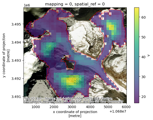
As a quick sanity check, we’ll convince ourselves that the clipping operation in the previous notebook worked correctly. We also show that we can plot both Xarray raster data and GeoPandas vector data overlaid on the same plot with a satellite image basemap as a background.
A few notes about the following figure:
single_glacier_rasteris a 3-dimensional object. We want to plot it in 2-d space with the RGI glacier outline. So, we perform a reduction (in this case, compute the mean), in order to reduce the dataset from 3-d to 2-d (Another option would be to select a single time step).We could make this plot with a white background, but it is also nice to be able to add a base map to the image. Here, we’ll use contextily to do so. This will require converting the coordinate reference system (CRS) of both objects to the Web Mercator projection (EPSG:3857). We first need to use
rio.write_crs()to assign a CRS to the raster object (Note: the data is already projected in the correct CRS, the object is just not ‘aware’ of its CRS. This is necessary for reprojection operations. For more, see Rioxarray’s CRS Management documentation).
#Write CRS of raster data
single_glacier_raster = single_glacier_raster.rio.write_crs(single_glacier_raster.attrs['projection'])
#Check that CRS of vector and raster data are the same
assert single_glacier_raster.rio.crs == single_glacier_vector.crs
#Reproject both objects to web mercator
single_glacier_vector_web = single_glacier_vector.to_crs('EPSG:3857')
single_glacier_raster_web = single_glacier_raster.rio.reproject('EPSG:3857')

fig, ax = plt.subplots(figsize=(8,5))

#Plot objects
single_glacier_raster_web.v.mean(dim='mid_date').plot(ax=ax, cmap='viridis', alpha=0.75, add_colorbar=True)
single_glacier_vector_web.plot(ax=ax, facecolor='None', edgecolor='red', alpha=0.75)
#Add basemap
cx.add_basemap(ax, crs=single_glacier_vector_web.crs, source=cx.providers.Esri.WorldImagery)
;
''
We sorted along the time dimension in the previous notebook, so it should be in chronological order.
single_glacier_raster.mid_date
<xarray.DataArray 'mid_date' (mid_date: 47892)> Size: 383kB
array(['1986-09-11T03:31:15.003252992', '1986-10-05T03:31:06.144750016',
       '1986-10-21T03:31:34.493249984', ..., '2024-10-29T04:18:09.241024000',
       '2024-10-29T04:18:09.241024000', '2024-10-29T04:18:09.241024000'],
      dtype='datetime64[ns]')
Coordinates:
    mapping      int64 8B 0
  * mid_date     (mid_date) datetime64[ns] 383kB 1986-09-11T03:31:15.00325299...
    spatial_ref  int64 8B 0
Attributes:
    description:    midpoint of image 1 and image 2 acquisition date and time...
standard_name: image_pair_center_date_with_time_separation- mid_date: 47892
- 1986-09-11T03:31:15.003252992 ... 2024-10-29T04:18:09.241024
array(['1986-09-11T03:31:15.003252992', '1986-10-05T03:31:06.144750016', '1986-10-21T03:31:34.493249984', ..., '2024-10-29T04:18:09.241024000', '2024-10-29T04:18:09.241024000', '2024-10-29T04:18:09.241024000'], dtype='datetime64[ns]') - mapping()int640
- crs_wkt :
- PROJCS["WGS 84 / UTM zone 46N",GEOGCS["WGS 84",DATUM["WGS_1984",SPHEROID["WGS 84",6378137,298.257223563]],PRIMEM["Greenwich",0],UNIT["degree",0.0174532925199433,AUTHORITY["EPSG","9122"]],AUTHORITY["EPSG","4326"]],PROJECTION["Transverse_Mercator"],PARAMETER["latitude_of_origin",0],PARAMETER["central_meridian",93],PARAMETER["scale_factor",0.9996],PARAMETER["false_easting",500000],PARAMETER["false_northing",0],UNIT["metre",1],AXIS["Easting",EAST],AXIS["Northing",NORTH],AUTHORITY["EPSG","32646"]]
- semi_major_axis :
- 6378137.0
- semi_minor_axis :
- 6356752.314245179
- inverse_flattening :
- 298.257223563
- reference_ellipsoid_name :
- WGS 84
- longitude_of_prime_meridian :
- 0.0
- prime_meridian_name :
- Greenwich
- geographic_crs_name :
- WGS 84
- horizontal_datum_name :
- World Geodetic System 1984
- projected_crs_name :
- WGS 84 / UTM zone 46N
- grid_mapping_name :
- transverse_mercator
- latitude_of_projection_origin :
- 0.0
- longitude_of_central_meridian :
- 93.0
- false_easting :
- 500000.0
- false_northing :
- 0.0
- scale_factor_at_central_meridian :
- 0.9996
- spatial_ref :
- PROJCS["WGS 84 / UTM zone 46N",GEOGCS["WGS 84",DATUM["WGS_1984",SPHEROID["WGS 84",6378137,298.257223563]],PRIMEM["Greenwich",0],UNIT["degree",0.0174532925199433,AUTHORITY["EPSG","9122"]],AUTHORITY["EPSG","4326"]],PROJECTION["Transverse_Mercator"],PARAMETER["latitude_of_origin",0],PARAMETER["central_meridian",93],PARAMETER["scale_factor",0.9996],PARAMETER["false_easting",500000],PARAMETER["false_northing",0],UNIT["metre",1],AXIS["Easting",EAST],AXIS["Northing",NORTH],AUTHORITY["EPSG","32646"]]
array(0)
- mid_date(mid_date)datetime64[ns]1986-09-11T03:31:15.003252992 .....
- description :
- midpoint of image 1 and image 2 acquisition date and time with granule's centroid longitude and latitude as microseconds
- standard_name :
- image_pair_center_date_with_time_separation
array(['1986-09-11T03:31:15.003252992', '1986-10-05T03:31:06.144750016', '1986-10-21T03:31:34.493249984', ..., '2024-10-29T04:18:09.241024000', '2024-10-29T04:18:09.241024000', '2024-10-29T04:18:09.241024000'], dtype='datetime64[ns]') - spatial_ref()int640
- GeoTransform :
- 784192.5 120.0 0.0 3315847.5 0.0 -120.0
array(0)
- mid_datePandasIndex
PandasIndex(DatetimeIndex(['1986-09-11 03:31:15.003252992',
               '1986-10-05 03:31:06.144750016',
               '1986-10-21 03:31:34.493249984',
               '1986-11-22 03:29:27.023556992',
               '1986-11-30 03:29:08.710132992',
               '1986-12-08 03:29:55.372057024',
               '1986-12-08 03:33:17.095283968',
                  '1986-12-16 03:30:10.645544',
               '1986-12-24 03:29:52.332120960',
               '1987-01-09 03:30:01.787228992',
               ...
               '2024-10-21 16:17:50.241008896',
               '2024-10-24 04:17:34.241014016',
               '2024-10-24 04:17:34.241014016',
               '2024-10-24 04:17:34.241014016',
               '2024-10-24 04:17:34.241014016',
               '2024-10-25 04:10:35.189837056',
                  '2024-10-29 04:18:09.241024',
                  '2024-10-29 04:18:09.241024',
                  '2024-10-29 04:18:09.241024',
                  '2024-10-29 04:18:09.241024'],
              dtype='datetime64[ns]', name='mid_date', length=47892, freq=None))
- description :
- midpoint of image 1 and image 2 acquisition date and time with granule's centroid longitude and latitude as microseconds
- standard_name :
- image_pair_center_date_with_time_separation
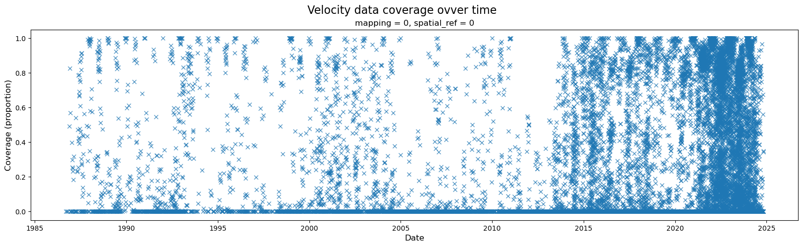
2) Examine data coverage#
A wide variety of forces can impact both satellite imagery and the ability of ITS_LIVE’s feature tracking algorithm to extract velocity estimates from satellite image pairs. For these reasons, there are at times both gaps in coverage and ranges in the estimated error associated with different observations. The following section will demonstrate how to calculate and visualize coverage of the dataset over time. Part 2 will include a discussion of uncertainty and error estimates
When first investigating a dataset, it is helpful to be able to scan/quickly visualize coverage along a given dimension. To create the data needed for such a visualization, we first need a mask that will tell us all possible ‘valid’ pixels; in other words, we need to differentiate between pixels in our 2-d rectangular array that represent ice v. non-ice. Then, for every time step, we can calculate the portion of possible ice pixels that contain an estimated velocity value.
#calculate number of valid pixels
valid_pixels = single_glacier_raster.v.count(dim=['x','y'])
#calculate max. number of valid pixels
valid_pixels_max = single_glacier_raster.v.notnull().any('mid_date').sum(['x','y'])
#add cov proportion to dataset as variable
single_glacier_raster['cov'] = valid_pixels/ valid_pixels_max
Now we can visualize coverage over time:
fig, ax = plt.subplots(figsize=(20,5))

#Plot object
single_glacier_raster['cov'].plot(ax=ax, linestyle='None', marker='x',alpha=0.75)

#Specify axes labels and title
fig.suptitle('Velocity data coverage ovver time', fontsize=16)
ax.set_ylabel('Coverage (proportion)', x=-0.05, fontsize=12)
ax.set_xlabel('Date', fontsize=12);
3) Break down by sensor#
In this dataset, we have a dense time series of velocity observations for a given glacier (~48,000 observatioons from 1986-2024 note: this notebook was last updated in 2025). However, we know that the ability of satellite imagery pairs to capture ice displacement (and by extension, velocity), can be impacted by conditions such as cloud-cover, which obscure Earth’s surface from optical sensors. ITS_LIVE is a multi-sensor ice velocity dataset, meaning that it is composed of ice velocity observations derived from a number of satellites, which include both optical and Synthetic Aperture Radar (SAR) imagery. Currently, Sentinel-1 is the only SAR sensor included in ITS_LIVE, all others are optical.
While optical imagery requires solar illumination and can be impacted by cloud cover, Sentinel-1 is an active remote sensing technique and images in a longer wavelength (C-band, ~ 5 cm). This means that Sentinel-1 imagery does not require solar illumination, and can penetrate through cloud cover. Because of these sensors differing sensitivity to Earth’s surface conditions, there can sometimes be discrapancies in velocity data observed from different sensors.
Note
There are many great resources available for understanding the principles of SAR and working with SAR imagery. The appendix at the bottom of this notebook lists a few of them. In addition, Chapter 2 of this tutorial focuses on working with a dataset of Sentinel-1 imagery.
Let’s first look at what sensors are represented in the time series:
sensors = list(set(single_glacier_raster.satellite_img1.values))
sensors
['5', '7', '2A', '8', '9', '2B', '1A', '4']
To extract observations from a single satellite sensor, we will use Xarray indexing and selection methods such as .where() and .sel(). The following cells demonstrate different selection approaches and a brief discussion of the pros and cons of each when working with large and/ or sparse datasets.
Landsat 8#
First, looking at velocity observations from Landsat8 data only:
%%time
l8_data = single_glacier_raster.where(single_glacier_raster['satellite_img1'] == '8', drop=True)
l8_data
CPU times: user 383 ms, sys: 3.54 s, total: 3.92 s
Wall time: 4.43 s
<xarray.Dataset> Size: 208MB
Dimensions:                     (mid_date: 2688, y: 37, x: 40)
Coordinates:
    mapping                     int64 8B 0
  * mid_date                    (mid_date) datetime64[ns] 22kB 2013-05-20T04:...
    spatial_ref                 int64 8B 0
  * x                           (x) float64 320B 7.843e+05 ... 7.889e+05
  * y                           (y) float64 296B 3.316e+06 ... 3.311e+06
Data variables: (12/60)
    M11                         (mid_date, y, x) float32 16MB nan nan ... nan
    M11_dr_to_vr_factor         (mid_date) float32 11kB nan nan nan ... nan nan
    M12                         (mid_date, y, x) float32 16MB nan nan ... nan
    M12_dr_to_vr_factor         (mid_date) float32 11kB nan nan nan ... nan nan
    acquisition_date_img1       (mid_date) datetime64[ns] 22kB 2013-04-30T04:...
    acquisition_date_img2       (mid_date) datetime64[ns] 22kB 2013-06-09T04:...
    ...                          ...
    vy_error_slow               (mid_date) float32 11kB 40.2 10.2 ... 26.5 159.6
    vy_error_stationary         (mid_date) float32 11kB 40.2 10.2 ... 26.5 159.6
    vy_stable_shift             (mid_date) float32 11kB -40.2 3.6 ... 17.1 152.1
    vy_stable_shift_slow        (mid_date) float32 11kB -40.2 3.6 ... 17.1 152.3
    vy_stable_shift_stationary  (mid_date) float32 11kB -40.2 3.6 ... 17.1 152.1
    cov                         (mid_date) float64 22kB 0.0 0.5969 ... 0.3494
Attributes: (12/19)
    Conventions:                CF-1.8
    GDAL_AREA_OR_POINT:         Area
    author:                     ITS_LIVE, a NASA MEaSUREs project (its-live.j...
    autoRIFT_parameter_file:    http://its-live-data.s3.amazonaws.com/autorif...
    datacube_software_version:  1.0
    date_created:               25-Sep-2023 22:00:23
    ...                         ...
    s3:                         s3://its-live-data/datacubes/v2/N30E090/ITS_L...
    skipped_granules:           s3://its-live-data/datacubes/v2/N30E090/ITS_L...
    time_standard_img1:         UTC
    time_standard_img2:         UTC
    title:                      ITS_LIVE datacube of image pair velocities
url: https://its-live-data.s3.amazonaws.com/datacu...- mid_date: 2688
- y: 37
- x: 40
- mapping()int640
- crs_wkt :
- PROJCS["WGS 84 / UTM zone 46N",GEOGCS["WGS 84",DATUM["WGS_1984",SPHEROID["WGS 84",6378137,298.257223563]],PRIMEM["Greenwich",0],UNIT["degree",0.0174532925199433,AUTHORITY["EPSG","9122"]],AUTHORITY["EPSG","4326"]],PROJECTION["Transverse_Mercator"],PARAMETER["latitude_of_origin",0],PARAMETER["central_meridian",93],PARAMETER["scale_factor",0.9996],PARAMETER["false_easting",500000],PARAMETER["false_northing",0],UNIT["metre",1],AXIS["Easting",EAST],AXIS["Northing",NORTH],AUTHORITY["EPSG","32646"]]
- semi_major_axis :
- 6378137.0
- semi_minor_axis :
- 6356752.314245179
- inverse_flattening :
- 298.257223563
- reference_ellipsoid_name :
- WGS 84
- longitude_of_prime_meridian :
- 0.0
- prime_meridian_name :
- Greenwich
- geographic_crs_name :
- WGS 84
- horizontal_datum_name :
- World Geodetic System 1984
- projected_crs_name :
- WGS 84 / UTM zone 46N
- grid_mapping_name :
- transverse_mercator
- latitude_of_projection_origin :
- 0.0
- longitude_of_central_meridian :
- 93.0
- false_easting :
- 500000.0
- false_northing :
- 0.0
- scale_factor_at_central_meridian :
- 0.9996
- spatial_ref :
- PROJCS["WGS 84 / UTM zone 46N",GEOGCS["WGS 84",DATUM["WGS_1984",SPHEROID["WGS 84",6378137,298.257223563]],PRIMEM["Greenwich",0],UNIT["degree",0.0174532925199433,AUTHORITY["EPSG","9122"]],AUTHORITY["EPSG","4326"]],PROJECTION["Transverse_Mercator"],PARAMETER["latitude_of_origin",0],PARAMETER["central_meridian",93],PARAMETER["scale_factor",0.9996],PARAMETER["false_easting",500000],PARAMETER["false_northing",0],UNIT["metre",1],AXIS["Easting",EAST],AXIS["Northing",NORTH],AUTHORITY["EPSG","32646"]]
array(0)
- mid_date(mid_date)datetime64[ns]2013-05-20T04:09:12.113346048 .....
- description :
- midpoint of image 1 and image 2 acquisition date and time with granule's centroid longitude and latitude as microseconds
- standard_name :
- image_pair_center_date_with_time_separation
array(['2013-05-20T04:09:12.113346048', '2013-06-17T04:12:21.907150080', '2013-06-21T04:08:58.673577984', ..., '2024-09-23T04:10:24.512207104', '2024-10-09T04:10:30.654570240', '2024-10-25T04:10:35.189837056'], dtype='datetime64[ns]') - spatial_ref()int640
- GeoTransform :
- 784192.5 120.0 0.0 3315847.5 0.0 -120.0
array(0)
- x(x)float647.843e+05 7.844e+05 ... 7.889e+05
- axis :
- X
- description :
- x coordinate of projection
- long_name :
- x coordinate of projection
- standard_name :
- projection_x_coordinate
- units :
- metre
array([784252.5, 784372.5, 784492.5, 784612.5, 784732.5, 784852.5, 784972.5, 785092.5, 785212.5, 785332.5, 785452.5, 785572.5, 785692.5, 785812.5, 785932.5, 786052.5, 786172.5, 786292.5, 786412.5, 786532.5, 786652.5, 786772.5, 786892.5, 787012.5, 787132.5, 787252.5, 787372.5, 787492.5, 787612.5, 787732.5, 787852.5, 787972.5, 788092.5, 788212.5, 788332.5, 788452.5, 788572.5, 788692.5, 788812.5, 788932.5]) - y(y)float643.316e+06 3.316e+06 ... 3.311e+06
- axis :
- Y
- description :
- y coordinate of projection
- long_name :
- y coordinate of projection
- standard_name :
- projection_y_coordinate
- units :
- metre
array([3315787.5, 3315667.5, 3315547.5, 3315427.5, 3315307.5, 3315187.5,
       3315067.5, 3314947.5, 3314827.5, 3314707.5, 3314587.5, 3314467.5,
       3314347.5, 3314227.5, 3314107.5, 3313987.5, 3313867.5, 3313747.5,
       3313627.5, 3313507.5, 3313387.5, 3313267.5, 3313147.5, 3313027.5,
       3312907.5, 3312787.5, 3312667.5, 3312547.5, 3312427.5, 3312307.5,
       3312187.5, 3312067.5, 3311947.5, 3311827.5, 3311707.5, 3311587.5,
       3311467.5])
- M11(mid_date, y, x)float32nan nan nan nan ... nan nan nan nan
- description :
- conversion matrix element (1st row, 1st column) that can be multiplied with vx to give range pixel displacement dr (see Eq. A18 in https://www.mdpi.com/2072-4292/13/4/749)
- standard_name :
- conversion_matrix_element_11
- units :
- pixel/(meter/year)
array([[[nan, nan, nan, ..., nan, nan, nan], [nan, nan, nan, ..., nan, nan, nan], [nan, nan, nan, ..., nan, nan, nan], ..., [nan, nan, nan, ..., nan, nan, nan], [nan, nan, nan, ..., nan, nan, nan], [nan, nan, nan, ..., nan, nan, nan]], [[nan, nan, nan, ..., nan, nan, nan], [nan, nan, nan, ..., nan, nan, nan], [nan, nan, nan, ..., nan, nan, nan], ..., [nan, nan, nan, ..., nan, nan, nan], [nan, nan, nan, ..., nan, nan, nan], [nan, nan, nan, ..., nan, nan, nan]], [[nan, nan, nan, ..., nan, nan, nan], [nan, nan, nan, ..., nan, nan, nan], [nan, nan, nan, ..., nan, nan, nan], ..., ... ..., [nan, nan, nan, ..., nan, nan, nan], [nan, nan, nan, ..., nan, nan, nan], [nan, nan, nan, ..., nan, nan, nan]], [[nan, nan, nan, ..., nan, nan, nan], [nan, nan, nan, ..., nan, nan, nan], [nan, nan, nan, ..., nan, nan, nan], ..., [nan, nan, nan, ..., nan, nan, nan], [nan, nan, nan, ..., nan, nan, nan], [nan, nan, nan, ..., nan, nan, nan]], [[nan, nan, nan, ..., nan, nan, nan], [nan, nan, nan, ..., nan, nan, nan], [nan, nan, nan, ..., nan, nan, nan], ..., [nan, nan, nan, ..., nan, nan, nan], [nan, nan, nan, ..., nan, nan, nan], [nan, nan, nan, ..., nan, nan, nan]]], dtype=float32) - M11_dr_to_vr_factor(mid_date)float32nan nan nan nan ... nan nan nan nan
- description :
- multiplicative factor that converts slant range pixel displacement dr to slant range velocity vr
- standard_name :
- M11_dr_to_vr_factor
- units :
- meter/(year*pixel)
array([nan, nan, nan, ..., nan, nan, nan], dtype=float32)
- M12(mid_date, y, x)float32nan nan nan nan ... nan nan nan nan
- description :
- conversion matrix element (1st row, 2nd column) that can be multiplied with vy to give range pixel displacement dr (see Eq. A18 in https://www.mdpi.com/2072-4292/13/4/749)
- standard_name :
- conversion_matrix_element_12
- units :
- pixel/(meter/year)
array([[[nan, nan, nan, ..., nan, nan, nan], [nan, nan, nan, ..., nan, nan, nan], [nan, nan, nan, ..., nan, nan, nan], ..., [nan, nan, nan, ..., nan, nan, nan], [nan, nan, nan, ..., nan, nan, nan], [nan, nan, nan, ..., nan, nan, nan]], [[nan, nan, nan, ..., nan, nan, nan], [nan, nan, nan, ..., nan, nan, nan], [nan, nan, nan, ..., nan, nan, nan], ..., [nan, nan, nan, ..., nan, nan, nan], [nan, nan, nan, ..., nan, nan, nan], [nan, nan, nan, ..., nan, nan, nan]], [[nan, nan, nan, ..., nan, nan, nan], [nan, nan, nan, ..., nan, nan, nan], [nan, nan, nan, ..., nan, nan, nan], ..., ... ..., [nan, nan, nan, ..., nan, nan, nan], [nan, nan, nan, ..., nan, nan, nan], [nan, nan, nan, ..., nan, nan, nan]], [[nan, nan, nan, ..., nan, nan, nan], [nan, nan, nan, ..., nan, nan, nan], [nan, nan, nan, ..., nan, nan, nan], ..., [nan, nan, nan, ..., nan, nan, nan], [nan, nan, nan, ..., nan, nan, nan], [nan, nan, nan, ..., nan, nan, nan]], [[nan, nan, nan, ..., nan, nan, nan], [nan, nan, nan, ..., nan, nan, nan], [nan, nan, nan, ..., nan, nan, nan], ..., [nan, nan, nan, ..., nan, nan, nan], [nan, nan, nan, ..., nan, nan, nan], [nan, nan, nan, ..., nan, nan, nan]]], dtype=float32) - M12_dr_to_vr_factor(mid_date)float32nan nan nan nan ... nan nan nan nan
- description :
- multiplicative factor that converts slant range pixel displacement dr to slant range velocity vr
- standard_name :
- M12_dr_to_vr_factor
- units :
- meter/(year*pixel)
array([nan, nan, nan, ..., nan, nan, nan], dtype=float32)
- acquisition_date_img1(mid_date)datetime64[ns]2013-04-30T04:12:14.819000064 .....
- description :
- acquisition date and time of image 1
- standard_name :
- image1_acquition_date
array(['2013-04-30T04:12:14.819000064', '2013-04-30T04:12:14.819000064', '2013-04-30T04:12:14.819000064', ..., '2024-08-18T04:10:11.608381696', '2024-09-19T04:10:23.892904960', '2024-10-21T04:10:32.963236096'], dtype='datetime64[ns]') - acquisition_date_img2(mid_date)datetime64[ns]2013-06-09T04:06:09.146831104 .....
- description :
- acquisition date and time of image 2
- standard_name :
- image2_acquition_date
array(['2013-06-09T04:06:09.146831104', '2013-08-04T04:12:28.734438912', '2013-08-12T04:05:42.267294976', ..., '2024-10-29T04:10:36.934395904', '2024-10-29T04:10:36.934395904', '2024-10-29T04:10:36.934395904'], dtype='datetime64[ns]') - autoRIFT_software_version(mid_date)object'1.5.0' '1.5.0' ... '1.5.0' '1.5.0'
- description :
- version of autoRIFT software
- standard_name :
- autoRIFT_software_version
array(['1.5.0', '1.5.0', '1.5.0', ..., '1.5.0', '1.5.0', '1.5.0'], dtype=object) - chip_size_height(mid_date, y, x)float32nan nan nan nan ... nan nan nan nan
- chip_size_coordinates :
- Optical data: chip_size_coordinates = 'image projection geometry: width = x, height = y'. Radar data: chip_size_coordinates = 'radar geometry: width = range, height = azimuth'
- description :
- height of search template (chip)
- standard_name :
- chip_size_height
- units :
- m
- y_pixel_size :
- 10.0
array([[[ nan, nan, nan, ..., nan, nan, nan], [ nan, nan, nan, ..., nan, nan, nan], [ nan, nan, nan, ..., nan, nan, nan], ..., [ nan, nan, nan, ..., nan, nan, nan], [ nan, nan, nan, ..., nan, nan, nan], [ nan, nan, nan, ..., nan, nan, nan]], [[ nan, nan, nan, ..., 240., nan, nan], [ nan, nan, nan, ..., 480., 240., nan], [ nan, nan, nan, ..., 480., 480., nan], ..., [ nan, nan, nan, ..., nan, nan, nan], [ nan, nan, nan, ..., nan, nan, nan], [ nan, nan, nan, ..., nan, nan, nan]], [[ nan, nan, nan, ..., nan, nan, nan], [ nan, nan, nan, ..., nan, nan, nan], [ nan, nan, nan, ..., nan, nan, nan], ..., ... ..., [ nan, nan, nan, ..., nan, nan, nan], [ nan, nan, nan, ..., nan, nan, nan], [ nan, nan, nan, ..., nan, nan, nan]], [[ nan, nan, nan, ..., nan, nan, nan], [ nan, nan, nan, ..., nan, nan, nan], [ nan, nan, nan, ..., nan, nan, nan], ..., [ nan, nan, nan, ..., nan, nan, nan], [ nan, nan, nan, ..., nan, nan, nan], [ nan, nan, nan, ..., nan, nan, nan]], [[ nan, nan, nan, ..., 480., nan, nan], [ nan, nan, nan, ..., 480., nan, nan], [ nan, nan, nan, ..., 480., nan, nan], ..., [ nan, nan, nan, ..., nan, nan, nan], [ nan, nan, nan, ..., nan, nan, nan], [ nan, nan, nan, ..., nan, nan, nan]]], dtype=float32) - chip_size_width(mid_date, y, x)float32nan nan nan nan ... nan nan nan nan
- chip_size_coordinates :
- Optical data: chip_size_coordinates = 'image projection geometry: width = x, height = y'. Radar data: chip_size_coordinates = 'radar geometry: width = range, height = azimuth'
- description :
- width of search template (chip)
- standard_name :
- chip_size_width
- units :
- m
- x_pixel_size :
- 10.0
array([[[ nan, nan, nan, ..., nan, nan, nan], [ nan, nan, nan, ..., nan, nan, nan], [ nan, nan, nan, ..., nan, nan, nan], ..., [ nan, nan, nan, ..., nan, nan, nan], [ nan, nan, nan, ..., nan, nan, nan], [ nan, nan, nan, ..., nan, nan, nan]], [[ nan, nan, nan, ..., 240., nan, nan], [ nan, nan, nan, ..., 480., 240., nan], [ nan, nan, nan, ..., 480., 480., nan], ..., [ nan, nan, nan, ..., nan, nan, nan], [ nan, nan, nan, ..., nan, nan, nan], [ nan, nan, nan, ..., nan, nan, nan]], [[ nan, nan, nan, ..., nan, nan, nan], [ nan, nan, nan, ..., nan, nan, nan], [ nan, nan, nan, ..., nan, nan, nan], ..., ... ..., [ nan, nan, nan, ..., nan, nan, nan], [ nan, nan, nan, ..., nan, nan, nan], [ nan, nan, nan, ..., nan, nan, nan]], [[ nan, nan, nan, ..., nan, nan, nan], [ nan, nan, nan, ..., nan, nan, nan], [ nan, nan, nan, ..., nan, nan, nan], ..., [ nan, nan, nan, ..., nan, nan, nan], [ nan, nan, nan, ..., nan, nan, nan], [ nan, nan, nan, ..., nan, nan, nan]], [[ nan, nan, nan, ..., 480., nan, nan], [ nan, nan, nan, ..., 480., nan, nan], [ nan, nan, nan, ..., 480., nan, nan], ..., [ nan, nan, nan, ..., nan, nan, nan], [ nan, nan, nan, ..., nan, nan, nan], [ nan, nan, nan, ..., nan, nan, nan]]], dtype=float32) - date_center(mid_date)datetime64[ns]2013-05-20T04:09:11.982916096 .....
- description :
- midpoint of image 1 and image 2 acquisition date
- standard_name :
- image_pair_center_date
array(['2013-05-20T04:09:11.982916096', '2013-06-17T04:12:21.776719872', '2013-06-21T04:08:58.543148032', ..., '2024-09-23T04:10:24.271388928', '2024-10-09T04:10:30.413650944', '2024-10-25T04:10:34.948815872'], dtype='datetime64[ns]') - date_dt(mid_date)timedelta64[ns]39 days 23:53:54.484863279 ... 8...
- description :
- time separation between acquisition of image 1 and image 2
- standard_name :
- image_pair_time_separation
array([3455634484863279, 8294413842773441, 8985207128906252, ..., 6220825048828126, 3456013183593747, 691203955078126], dtype='timedelta64[ns]') - floatingice(y, x, mid_date)float32nan nan nan nan ... nan nan nan nan
- description :
- floating ice mask, 0 = non-floating-ice, 1 = floating-ice
- flag_meanings :
- non-ice ice
- flag_values :
- [0, 1]
- standard_name :
- floating ice mask
- url :
- https://its-live-data.s3.amazonaws.com/autorift_parameters/v001/N46_0120m_floatingice.tif
array([[[nan, nan, nan, ..., nan, nan, nan], [nan, nan, nan, ..., nan, nan, nan], [nan, nan, nan, ..., nan, nan, nan], ..., [ 0., 0., 0., ..., 0., 0., 0.], [nan, nan, nan, ..., nan, nan, nan], [nan, nan, nan, ..., nan, nan, nan]], [[nan, nan, nan, ..., nan, nan, nan], [nan, nan, nan, ..., nan, nan, nan], [nan, nan, nan, ..., nan, nan, nan], ..., [ 0., 0., 0., ..., 0., 0., 0.], [ 0., 0., 0., ..., 0., 0., 0.], [nan, nan, nan, ..., nan, nan, nan]], [[nan, nan, nan, ..., nan, nan, nan], [nan, nan, nan, ..., nan, nan, nan], [nan, nan, nan, ..., nan, nan, nan], ..., ... ..., [nan, nan, nan, ..., nan, nan, nan], [nan, nan, nan, ..., nan, nan, nan], [nan, nan, nan, ..., nan, nan, nan]], [[nan, nan, nan, ..., nan, nan, nan], [nan, nan, nan, ..., nan, nan, nan], [nan, nan, nan, ..., nan, nan, nan], ..., [nan, nan, nan, ..., nan, nan, nan], [nan, nan, nan, ..., nan, nan, nan], [nan, nan, nan, ..., nan, nan, nan]], [[nan, nan, nan, ..., nan, nan, nan], [nan, nan, nan, ..., nan, nan, nan], [nan, nan, nan, ..., nan, nan, nan], ..., [nan, nan, nan, ..., nan, nan, nan], [nan, nan, nan, ..., nan, nan, nan], [nan, nan, nan, ..., nan, nan, nan]]], dtype=float32) - granule_url(mid_date)object'https://its-live-data.s3.amazon...
- description :
- original granule URL
- standard_name :
- granule_url
array(['https://its-live-data.s3.amazonaws.com/velocity_image_pair/landsatOLI/v02/N30E090/LC08_L1TP_135039_20130430_20200913_02_T1_X_LE07_L1TP_135039_20130609_20200907_02_T1_G0120V02_P012.nc', 'https://its-live-data.s3.amazonaws.com/velocity_image_pair/landsatOLI/v02/N30E090/LC08_L1TP_135039_20130430_20200913_02_T1_X_LC08_L1TP_135039_20130804_20200912_02_T1_G0120V02_P024.nc', 'https://its-live-data.s3.amazonaws.com/velocity_image_pair/landsatOLI/v02/N30E090/LC08_L1TP_135039_20130430_20200913_02_T1_X_LE07_L1TP_135039_20130812_20200907_02_T1_G0120V02_P029.nc', ..., 'https://its-live-data.s3.amazonaws.com/velocity_image_pair/landsatOLI/v02/N30E090/LC08_L1TP_135039_20240818_20240823_02_T1_X_LC09_L1TP_135039_20241029_20241029_02_T1_G0120V02_P014.nc', 'https://its-live-data.s3.amazonaws.com/velocity_image_pair/landsatOLI/v02/N30E090/LC08_L1TP_135039_20240919_20240927_02_T1_X_LC09_L1TP_135039_20241029_20241029_02_T1_G0120V02_P012.nc', 'https://its-live-data.s3.amazonaws.com/velocity_image_pair/landsatOLI/v02/N30E090/LC08_L1TP_135039_20241021_20241029_02_T1_X_LC09_L1TP_135039_20241029_20241029_02_T1_G0120V02_P020.nc'], dtype=object) - interp_mask(mid_date, y, x)float32nan nan nan nan ... nan nan nan nan
- description :
- light interpolation mask
- flag_meanings :
- measured interpolated
- flag_values :
- [0, 1]
- standard_name :
- interpolated_value_mask
array([[[nan, nan, nan, ..., nan, nan, nan], [nan, nan, nan, ..., nan, nan, nan], [nan, nan, nan, ..., nan, nan, nan], ..., [nan, nan, nan, ..., nan, nan, nan], [nan, nan, nan, ..., nan, nan, nan], [nan, nan, nan, ..., nan, nan, nan]], [[nan, nan, nan, ..., nan, nan, nan], [nan, nan, nan, ..., 1., nan, nan], [nan, nan, nan, ..., 1., 1., nan], ..., [nan, nan, nan, ..., nan, nan, nan], [nan, nan, nan, ..., nan, nan, nan], [nan, nan, nan, ..., nan, nan, nan]], [[nan, nan, nan, ..., nan, nan, nan], [nan, nan, nan, ..., nan, nan, nan], [nan, nan, nan, ..., nan, nan, nan], ..., ... ..., [nan, nan, nan, ..., nan, nan, nan], [nan, nan, nan, ..., nan, nan, nan], [nan, nan, nan, ..., nan, nan, nan]], [[nan, nan, nan, ..., nan, nan, nan], [nan, nan, nan, ..., nan, nan, nan], [nan, nan, nan, ..., nan, nan, nan], ..., [nan, nan, nan, ..., nan, nan, nan], [nan, nan, nan, ..., nan, nan, nan], [nan, nan, nan, ..., nan, nan, nan]], [[nan, nan, nan, ..., 1., nan, nan], [nan, nan, nan, ..., nan, nan, nan], [nan, nan, nan, ..., nan, nan, nan], ..., [nan, nan, nan, ..., nan, nan, nan], [nan, nan, nan, ..., nan, nan, nan], [nan, nan, nan, ..., nan, nan, nan]]], dtype=float32) - landice(y, x, mid_date)float32nan nan nan nan ... nan nan nan nan
- description :
- land ice mask, 0 = non-land-ice, 1 = land-ice
- flag_meanings :
- non-ice ice
- flag_values :
- [0, 1]
- standard_name :
- land ice mask
- url :
- https://its-live-data.s3.amazonaws.com/autorift_parameters/v001/N46_0120m_landice.tif
array([[[nan, nan, nan, ..., nan, nan, nan], [nan, nan, nan, ..., nan, nan, nan], [nan, nan, nan, ..., nan, nan, nan], ..., [ 1., 1., 1., ..., 1., 1., 1.], [nan, nan, nan, ..., nan, nan, nan], [nan, nan, nan, ..., nan, nan, nan]], [[nan, nan, nan, ..., nan, nan, nan], [nan, nan, nan, ..., nan, nan, nan], [nan, nan, nan, ..., nan, nan, nan], ..., [ 1., 1., 1., ..., 1., 1., 1.], [ 1., 1., 1., ..., 1., 1., 1.], [nan, nan, nan, ..., nan, nan, nan]], [[nan, nan, nan, ..., nan, nan, nan], [nan, nan, nan, ..., nan, nan, nan], [nan, nan, nan, ..., nan, nan, nan], ..., ... ..., [nan, nan, nan, ..., nan, nan, nan], [nan, nan, nan, ..., nan, nan, nan], [nan, nan, nan, ..., nan, nan, nan]], [[nan, nan, nan, ..., nan, nan, nan], [nan, nan, nan, ..., nan, nan, nan], [nan, nan, nan, ..., nan, nan, nan], ..., [nan, nan, nan, ..., nan, nan, nan], [nan, nan, nan, ..., nan, nan, nan], [nan, nan, nan, ..., nan, nan, nan]], [[nan, nan, nan, ..., nan, nan, nan], [nan, nan, nan, ..., nan, nan, nan], [nan, nan, nan, ..., nan, nan, nan], ..., [nan, nan, nan, ..., nan, nan, nan], [nan, nan, nan, ..., nan, nan, nan], [nan, nan, nan, ..., nan, nan, nan]]], dtype=float32) - mission_img1(mid_date)object'L' 'L' 'L' 'L' ... 'L' 'L' 'L' 'L'
- description :
- id of the mission that acquired image 1
- standard_name :
- image1_mission
array(['L', 'L', 'L', ..., 'L', 'L', 'L'], dtype=object)
- mission_img2(mid_date)object'L' 'L' 'L' 'L' ... 'L' 'L' 'L' 'L'
- description :
- id of the mission that acquired image 2
- standard_name :
- image2_mission
array(['L', 'L', 'L', ..., 'L', 'L', 'L'], dtype=object)
- roi_valid_percentage(mid_date)float3212.6 24.4 29.9 ... 14.8 12.4 20.6
- description :
- percentage of pixels with a valid velocity estimate determined for the intersection of the full image pair footprint and the region of interest (roi) that defines where autoRIFT tried to estimate a velocity
- standard_name :
- region_of_interest_valid_pixel_percentage
array([12.6, 24.4, 29.9, ..., 14.8, 12.4, 20.6], dtype=float32)
- satellite_img1(mid_date)object'8' '8' '8' '8' ... '8' '8' '8' '8'
- description :
- id of the satellite that acquired image 1
- standard_name :
- image1_satellite
array(['8', '8', '8', ..., '8', '8', '8'], dtype=object)
- satellite_img2(mid_date)object'7' '8' '7' '8' ... '9' '9' '9' '9'
- description :
- id of the satellite that acquired image 2
- standard_name :
- image2_satellite
array(['7', '8', '7', ..., '9', '9', '9'], dtype=object)
- sensor_img1(mid_date)object'C' 'C' 'C' 'C' ... 'C' 'C' 'C' 'C'
- description :
- id of the sensor that acquired image 1
- standard_name :
- image1_sensor
array(['C', 'C', 'C', ..., 'C', 'C', 'C'], dtype=object)
- sensor_img2(mid_date)object'E' 'C' 'E' 'C' ... 'C' 'C' 'C' 'C'
- description :
- id of the sensor that acquired image 2
- standard_name :
- image2_sensor
array(['E', 'C', 'E', ..., 'C', 'C', 'C'], dtype=object)
- stable_count_slow(mid_date)float324.055e+04 4.19e+04 ... 7.394e+03
- description :
- number of valid pixels over slowest 25% of ice
- standard_name :
- stable_count_slow
- units :
- count
array([40553., 41895., 51511., ..., 44733., 59503., 7394.], dtype=float32)
- stable_count_stationary(mid_date)float323.967e+04 4.009e+04 ... 4.764e+03
- description :
- number of valid pixels over stationary or slow-flowing surfaces
- standard_name :
- stable_count_stationary
- units :
- count
array([39668., 40088., 49258., ..., 42886., 58153., 4764.], dtype=float32)
- stable_shift_flag(mid_date)float321.0 1.0 1.0 1.0 ... 1.0 1.0 1.0 1.0
- description :
- flag for applying velocity bias correction: 0 = no correction; 1 = correction from overlapping stable surface mask (stationary or slow-flowing surfaces with velocity < 15 m/yr)(top priority); 2 = correction from slowest 25% of overlapping velocities (second priority)
- standard_name :
- stable_shift_flag
array([1., 1., 1., ..., 1., 1., 1.], dtype=float32)
- v(mid_date, y, x)float32nan nan nan nan ... nan nan nan nan
- description :
- velocity magnitude
- standard_name :
- land_ice_surface_velocity
- units :
- meter/year
array([[[ nan, nan, nan, ..., nan, nan, nan], [ nan, nan, nan, ..., nan, nan, nan], [ nan, nan, nan, ..., nan, nan, nan], ..., [ nan, nan, nan, ..., nan, nan, nan], [ nan, nan, nan, ..., nan, nan, nan], [ nan, nan, nan, ..., nan, nan, nan]], [[ nan, nan, nan, ..., 7., nan, nan], [ nan, nan, nan, ..., 2., 23., nan], [ nan, nan, nan, ..., 4., 2., nan], ..., [ nan, nan, nan, ..., nan, nan, nan], [ nan, nan, nan, ..., nan, nan, nan], [ nan, nan, nan, ..., nan, nan, nan]], [[ nan, nan, nan, ..., nan, nan, nan], [ nan, nan, nan, ..., nan, nan, nan], [ nan, nan, nan, ..., nan, nan, nan], ..., ... ..., [ nan, nan, nan, ..., nan, nan, nan], [ nan, nan, nan, ..., nan, nan, nan], [ nan, nan, nan, ..., nan, nan, nan]], [[ nan, nan, nan, ..., nan, nan, nan], [ nan, nan, nan, ..., nan, nan, nan], [ nan, nan, nan, ..., nan, nan, nan], ..., [ nan, nan, nan, ..., nan, nan, nan], [ nan, nan, nan, ..., nan, nan, nan], [ nan, nan, nan, ..., nan, nan, nan]], [[ nan, nan, nan, ..., 72., nan, nan], [ nan, nan, nan, ..., 161., nan, nan], [ nan, nan, nan, ..., 158., nan, nan], ..., [ nan, nan, nan, ..., nan, nan, nan], [ nan, nan, nan, ..., nan, nan, nan], [ nan, nan, nan, ..., nan, nan, nan]]], dtype=float32) - v_error(mid_date, y, x)float32nan nan nan nan ... nan nan nan nan
- description :
- velocity magnitude error
- standard_name :
- velocity_error
- units :
- meter/year
array([[[ nan, nan, nan, ..., nan, nan, nan], [ nan, nan, nan, ..., nan, nan, nan], [ nan, nan, nan, ..., nan, nan, nan], ..., [ nan, nan, nan, ..., nan, nan, nan], [ nan, nan, nan, ..., nan, nan, nan], [ nan, nan, nan, ..., nan, nan, nan]], [[ nan, nan, nan, ..., 10., nan, nan], [ nan, nan, nan, ..., 10., 10., nan], [ nan, nan, nan, ..., 10., 10., nan], ..., [ nan, nan, nan, ..., nan, nan, nan], [ nan, nan, nan, ..., nan, nan, nan], [ nan, nan, nan, ..., nan, nan, nan]], [[ nan, nan, nan, ..., nan, nan, nan], [ nan, nan, nan, ..., nan, nan, nan], [ nan, nan, nan, ..., nan, nan, nan], ..., ... ..., [ nan, nan, nan, ..., nan, nan, nan], [ nan, nan, nan, ..., nan, nan, nan], [ nan, nan, nan, ..., nan, nan, nan]], [[ nan, nan, nan, ..., nan, nan, nan], [ nan, nan, nan, ..., nan, nan, nan], [ nan, nan, nan, ..., nan, nan, nan], ..., [ nan, nan, nan, ..., nan, nan, nan], [ nan, nan, nan, ..., nan, nan, nan], [ nan, nan, nan, ..., nan, nan, nan]], [[ nan, nan, nan, ..., 143., nan, nan], [ nan, nan, nan, ..., 113., nan, nan], [ nan, nan, nan, ..., 112., nan, nan], ..., [ nan, nan, nan, ..., nan, nan, nan], [ nan, nan, nan, ..., nan, nan, nan], [ nan, nan, nan, ..., nan, nan, nan]]], dtype=float32) - va(mid_date, y, x)float32nan nan nan nan ... nan nan nan nan
- description :
- velocity in radar azimuth direction
array([[[nan, nan, nan, ..., nan, nan, nan], [nan, nan, nan, ..., nan, nan, nan], [nan, nan, nan, ..., nan, nan, nan], ..., [nan, nan, nan, ..., nan, nan, nan], [nan, nan, nan, ..., nan, nan, nan], [nan, nan, nan, ..., nan, nan, nan]], [[nan, nan, nan, ..., nan, nan, nan], [nan, nan, nan, ..., nan, nan, nan], [nan, nan, nan, ..., nan, nan, nan], ..., [nan, nan, nan, ..., nan, nan, nan], [nan, nan, nan, ..., nan, nan, nan], [nan, nan, nan, ..., nan, nan, nan]], [[nan, nan, nan, ..., nan, nan, nan], [nan, nan, nan, ..., nan, nan, nan], [nan, nan, nan, ..., nan, nan, nan], ..., ... ..., [nan, nan, nan, ..., nan, nan, nan], [nan, nan, nan, ..., nan, nan, nan], [nan, nan, nan, ..., nan, nan, nan]], [[nan, nan, nan, ..., nan, nan, nan], [nan, nan, nan, ..., nan, nan, nan], [nan, nan, nan, ..., nan, nan, nan], ..., [nan, nan, nan, ..., nan, nan, nan], [nan, nan, nan, ..., nan, nan, nan], [nan, nan, nan, ..., nan, nan, nan]], [[nan, nan, nan, ..., nan, nan, nan], [nan, nan, nan, ..., nan, nan, nan], [nan, nan, nan, ..., nan, nan, nan], ..., [nan, nan, nan, ..., nan, nan, nan], [nan, nan, nan, ..., nan, nan, nan], [nan, nan, nan, ..., nan, nan, nan]]], dtype=float32) - va_error(mid_date)float32nan nan nan nan ... nan nan nan nan
- description :
- error for velocity in radar azimuth direction
- standard_name :
- va_error
- units :
- meter/year
array([nan, nan, nan, ..., nan, nan, nan], dtype=float32)
- va_error_modeled(mid_date)float32nan nan nan nan ... nan nan nan nan
- description :
- 1-sigma error calculated using a modeled error-dt relationship
- standard_name :
- va_error_modeled
- units :
- meter/year
array([nan, nan, nan, ..., nan, nan, nan], dtype=float32)
- va_error_slow(mid_date)float32nan nan nan nan ... nan nan nan nan
- description :
- RMSE over slowest 25% of retrieved velocities
- standard_name :
- va_error_slow
- units :
- meter/year
array([nan, nan, nan, ..., nan, nan, nan], dtype=float32)
- va_error_stationary(mid_date)float32nan nan nan nan ... nan nan nan nan
- description :
- RMSE over stable surfaces, stationary or slow-flowing surfaces with velocity < 15 m/yr identified from an external mask
- standard_name :
- va_error_stationary
- units :
- meter/year
array([nan, nan, nan, ..., nan, nan, nan], dtype=float32)
- va_stable_shift(mid_date)float32nan nan nan nan ... nan nan nan nan
- description :
- applied va shift calibrated using pixels over stable or slow surfaces
- standard_name :
- va_stable_shift
- units :
- meter/year
array([nan, nan, nan, ..., nan, nan, nan], dtype=float32)
- va_stable_shift_slow(mid_date)float32nan nan nan nan ... nan nan nan nan
- description :
- va shift calibrated using valid pixels over slowest 25% of retrieved velocities
- standard_name :
- va_stable_shift_slow
- units :
- meter/year
array([nan, nan, nan, ..., nan, nan, nan], dtype=float32)
- va_stable_shift_stationary(mid_date)float32nan nan nan nan ... nan nan nan nan
- description :
- va shift calibrated using valid pixels over stable surfaces, stationary or slow-flowing surfaces with velocity < 15 m/yr identified from an external mask
- standard_name :
- va_stable_shift_stationary
- units :
- meter/year
array([nan, nan, nan, ..., nan, nan, nan], dtype=float32)
- vr(mid_date, y, x)float32nan nan nan nan ... nan nan nan nan
- description :
- velocity in radar range direction
array([[[nan, nan, nan, ..., nan, nan, nan], [nan, nan, nan, ..., nan, nan, nan], [nan, nan, nan, ..., nan, nan, nan], ..., [nan, nan, nan, ..., nan, nan, nan], [nan, nan, nan, ..., nan, nan, nan], [nan, nan, nan, ..., nan, nan, nan]], [[nan, nan, nan, ..., nan, nan, nan], [nan, nan, nan, ..., nan, nan, nan], [nan, nan, nan, ..., nan, nan, nan], ..., [nan, nan, nan, ..., nan, nan, nan], [nan, nan, nan, ..., nan, nan, nan], [nan, nan, nan, ..., nan, nan, nan]], [[nan, nan, nan, ..., nan, nan, nan], [nan, nan, nan, ..., nan, nan, nan], [nan, nan, nan, ..., nan, nan, nan], ..., ... ..., [nan, nan, nan, ..., nan, nan, nan], [nan, nan, nan, ..., nan, nan, nan], [nan, nan, nan, ..., nan, nan, nan]], [[nan, nan, nan, ..., nan, nan, nan], [nan, nan, nan, ..., nan, nan, nan], [nan, nan, nan, ..., nan, nan, nan], ..., [nan, nan, nan, ..., nan, nan, nan], [nan, nan, nan, ..., nan, nan, nan], [nan, nan, nan, ..., nan, nan, nan]], [[nan, nan, nan, ..., nan, nan, nan], [nan, nan, nan, ..., nan, nan, nan], [nan, nan, nan, ..., nan, nan, nan], ..., [nan, nan, nan, ..., nan, nan, nan], [nan, nan, nan, ..., nan, nan, nan], [nan, nan, nan, ..., nan, nan, nan]]], dtype=float32) - vr_error(mid_date)float32nan nan nan nan ... nan nan nan nan
- description :
- error for velocity in radar range direction
- standard_name :
- vr_error
- units :
- meter/year
array([nan, nan, nan, ..., nan, nan, nan], dtype=float32)
- vr_error_modeled(mid_date)float32nan nan nan nan ... nan nan nan nan
- description :
- 1-sigma error calculated using a modeled error-dt relationship
- standard_name :
- vr_error_modeled
- units :
- meter/year
array([nan, nan, nan, ..., nan, nan, nan], dtype=float32)
- vr_error_slow(mid_date)float32nan nan nan nan ... nan nan nan nan
- description :
- RMSE over slowest 25% of retrieved velocities
- standard_name :
- vr_error_slow
- units :
- meter/year
array([nan, nan, nan, ..., nan, nan, nan], dtype=float32)
- vr_error_stationary(mid_date)float32nan nan nan nan ... nan nan nan nan
- description :
- RMSE over stable surfaces, stationary or slow-flowing surfaces with velocity < 15 m/yr identified from an external mask
- standard_name :
- vr_error_stationary
- units :
- meter/year
array([nan, nan, nan, ..., nan, nan, nan], dtype=float32)
- vr_stable_shift(mid_date)float32nan nan nan nan ... nan nan nan nan
- description :
- applied vr shift calibrated using pixels over stable or slow surfaces
- standard_name :
- vr_stable_shift
- units :
- meter/year
array([nan, nan, nan, ..., nan, nan, nan], dtype=float32)
- vr_stable_shift_slow(mid_date)float32nan nan nan nan ... nan nan nan nan
- description :
- vr shift calibrated using valid pixels over slowest 25% of retrieved velocities
- standard_name :
- vr_stable_shift_slow
- units :
- meter/year
array([nan, nan, nan, ..., nan, nan, nan], dtype=float32)
- vr_stable_shift_stationary(mid_date)float32nan nan nan nan ... nan nan nan nan
- description :
- vr shift calibrated using valid pixels over stable surfaces, stationary or slow-flowing surfaces with velocity < 15 m/yr identified from an external mask
- standard_name :
- vr_stable_shift_stationary
- units :
- meter/year
array([nan, nan, nan, ..., nan, nan, nan], dtype=float32)
- vx(mid_date, y, x)float32nan nan nan nan ... nan nan nan nan
- description :
- velocity component in x direction
- standard_name :
- land_ice_surface_x_velocity
- units :
- meter/year
array([[[ nan, nan, nan, ..., nan, nan, nan], [ nan, nan, nan, ..., nan, nan, nan], [ nan, nan, nan, ..., nan, nan, nan], ..., [ nan, nan, nan, ..., nan, nan, nan], [ nan, nan, nan, ..., nan, nan, nan], [ nan, nan, nan, ..., nan, nan, nan]], [[ nan, nan, nan, ..., 0., nan, nan], [ nan, nan, nan, ..., -2., -7., nan], [ nan, nan, nan, ..., -3., 1., nan], ..., [ nan, nan, nan, ..., nan, nan, nan], [ nan, nan, nan, ..., nan, nan, nan], [ nan, nan, nan, ..., nan, nan, nan]], [[ nan, nan, nan, ..., nan, nan, nan], [ nan, nan, nan, ..., nan, nan, nan], [ nan, nan, nan, ..., nan, nan, nan], ..., ... ..., [ nan, nan, nan, ..., nan, nan, nan], [ nan, nan, nan, ..., nan, nan, nan], [ nan, nan, nan, ..., nan, nan, nan]], [[ nan, nan, nan, ..., nan, nan, nan], [ nan, nan, nan, ..., nan, nan, nan], [ nan, nan, nan, ..., nan, nan, nan], ..., [ nan, nan, nan, ..., nan, nan, nan], [ nan, nan, nan, ..., nan, nan, nan], [ nan, nan, nan, ..., nan, nan, nan]], [[ nan, nan, nan, ..., 41., nan, nan], [ nan, nan, nan, ..., 147., nan, nan], [ nan, nan, nan, ..., 145., nan, nan], ..., [ nan, nan, nan, ..., nan, nan, nan], [ nan, nan, nan, ..., nan, nan, nan], [ nan, nan, nan, ..., nan, nan, nan]]], dtype=float32) - vx_error(mid_date)float3278.2 9.5 24.5 ... 11.8 17.5 100.5
- description :
- best estimate of x_velocity error: vx_error is populated according to the approach used for the velocity bias correction as indicated in "stable_shift_flag"
- standard_name :
- vx_error
- units :
- meter/year
array([ 78.2, 9.5, 24.5, ..., 11.8, 17.5, 100.5], dtype=float32)
- vx_error_modeled(mid_date)float32232.7 97.0 89.5 ... 232.7 1.163e+03
- description :
- 1-sigma error calculated using a modeled error-dt relationship
- standard_name :
- vx_error_modeled
- units :
- meter/year
array([ 232.7, 97. , 89.5, ..., 129.3, 232.7, 1163.4], dtype=float32)
- vx_error_slow(mid_date)float3278.2 9.5 24.5 ... 11.8 17.5 100.4
- description :
- RMSE over slowest 25% of retrieved velocities
- standard_name :
- vx_error_slow
- units :
- meter/year
array([ 78.2, 9.5, 24.5, ..., 11.8, 17.5, 100.4], dtype=float32)
- vx_error_stationary(mid_date)float3278.2 9.5 24.5 ... 11.8 17.5 100.5
- description :
- RMSE over stable surfaces, stationary or slow-flowing surfaces with velocity < 15 meter/year identified from an external mask
- standard_name :
- vx_error_stationary
- units :
- meter/year
array([ 78.2, 9.5, 24.5, ..., 11.8, 17.5, 100.5], dtype=float32)
- vx_stable_shift(mid_date)float3256.9 0.0 3.3 0.0 ... 0.1 0.0 -21.6
- description :
- applied vx shift calibrated using pixels over stable or slow surfaces
- standard_name :
- vx_stable_shift
- units :
- meter/year
array([ 56.9, 0. , 3.3, ..., 0.1, 0. , -21.6], dtype=float32)
- vx_stable_shift_slow(mid_date)float3257.3 0.0 3.3 0.0 ... 0.1 0.0 -21.6
- description :
- vx shift calibrated using valid pixels over slowest 25% of retrieved velocities
- standard_name :
- vx_stable_shift_slow
- units :
- meter/year
array([ 57.3, 0. , 3.3, ..., 0.1, 0. , -21.6], dtype=float32)
- vx_stable_shift_stationary(mid_date)float3256.9 0.0 3.3 0.0 ... 0.1 0.0 -21.6
- description :
- vx shift calibrated using valid pixels over stable surfaces, stationary or slow-flowing surfaces with velocity < 15 m/yr identified from an external mask
- standard_name :
- vx_stable_shift_stationary
- units :
- meter/year
array([ 56.9, 0. , 3.3, ..., 0.1, 0. , -21.6], dtype=float32)
- vy(mid_date, y, x)float32nan nan nan nan ... nan nan nan nan
- description :
- velocity component in y direction
- standard_name :
- land_ice_surface_y_velocity
- units :
- meter/year
array([[[nan, nan, nan, ..., nan, nan, nan], [nan, nan, nan, ..., nan, nan, nan], [nan, nan, nan, ..., nan, nan, nan], ..., [nan, nan, nan, ..., nan, nan, nan], [nan, nan, nan, ..., nan, nan, nan], [nan, nan, nan, ..., nan, nan, nan]], [[nan, nan, nan, ..., -7., nan, nan], [nan, nan, nan, ..., -1., 21., nan], [nan, nan, nan, ..., -2., -2., nan], ..., [nan, nan, nan, ..., nan, nan, nan], [nan, nan, nan, ..., nan, nan, nan], [nan, nan, nan, ..., nan, nan, nan]], [[nan, nan, nan, ..., nan, nan, nan], [nan, nan, nan, ..., nan, nan, nan], [nan, nan, nan, ..., nan, nan, nan], ..., ... ..., [nan, nan, nan, ..., nan, nan, nan], [nan, nan, nan, ..., nan, nan, nan], [nan, nan, nan, ..., nan, nan, nan]], [[nan, nan, nan, ..., nan, nan, nan], [nan, nan, nan, ..., nan, nan, nan], [nan, nan, nan, ..., nan, nan, nan], ..., [nan, nan, nan, ..., nan, nan, nan], [nan, nan, nan, ..., nan, nan, nan], [nan, nan, nan, ..., nan, nan, nan]], [[nan, nan, nan, ..., 59., nan, nan], [nan, nan, nan, ..., 67., nan, nan], [nan, nan, nan, ..., 62., nan, nan], ..., [nan, nan, nan, ..., nan, nan, nan], [nan, nan, nan, ..., nan, nan, nan], [nan, nan, nan, ..., nan, nan, nan]]], dtype=float32) - vy_error(mid_date)float3240.2 10.2 15.1 ... 16.8 26.5 159.6
- description :
- best estimate of y_velocity error: vy_error is populated according to the approach used for the velocity bias correction as indicated in "stable_shift_flag"
- standard_name :
- vy_error
- units :
- meter/year
array([ 40.2, 10.2, 15.1, ..., 16.8, 26.5, 159.6], dtype=float32)
- vy_error_modeled(mid_date)float32232.7 97.0 89.5 ... 232.7 1.163e+03
- description :
- 1-sigma error calculated using a modeled error-dt relationship
- standard_name :
- vy_error_modeled
- units :
- meter/year
array([ 232.7, 97. , 89.5, ..., 129.3, 232.7, 1163.4], dtype=float32)
- vy_error_slow(mid_date)float3240.2 10.2 15.1 ... 16.8 26.5 159.6
- description :
- RMSE over slowest 25% of retrieved velocities
- standard_name :
- vy_error_slow
- units :
- meter/year
array([ 40.2, 10.2, 15.1, ..., 16.8, 26.5, 159.6], dtype=float32)
- vy_error_stationary(mid_date)float3240.2 10.2 15.1 ... 16.8 26.5 159.6
- description :
- RMSE over stable surfaces, stationary or slow-flowing surfaces with velocity < 15 meter/year identified from an external mask
- standard_name :
- vy_error_stationary
- units :
- meter/year
array([ 40.2, 10.2, 15.1, ..., 16.8, 26.5, 159.6], dtype=float32)
- vy_stable_shift(mid_date)float32-40.2 3.6 3.3 ... 4.7 17.1 152.1
- description :
- applied vy shift calibrated using pixels over stable or slow surfaces
- standard_name :
- vy_stable_shift
- units :
- meter/year
array([-40.2, 3.6, 3.3, ..., 4.7, 17.1, 152.1], dtype=float32)
- vy_stable_shift_slow(mid_date)float32-40.2 3.6 3.3 ... 4.7 17.1 152.3
- description :
- vy shift calibrated using valid pixels over slowest 25% of retrieved velocities
- standard_name :
- vy_stable_shift_slow
- units :
- meter/year
array([-40.2, 3.6, 3.3, ..., 4.7, 17.1, 152.3], dtype=float32)
- vy_stable_shift_stationary(mid_date)float32-40.2 3.6 3.3 ... 4.7 17.1 152.1
- description :
- vy shift calibrated using valid pixels over stable surfaces, stationary or slow-flowing surfaces with velocity < 15 m/yr identified from an external mask
- standard_name :
- vy_stable_shift_stationary
- units :
- meter/year
array([-40.2, 3.6, 3.3, ..., 4.7, 17.1, 152.1], dtype=float32)
- cov(mid_date)float640.0 0.5969 0.05092 ... 0.0 0.3494
array([0.        , 0.59688826, 0.05091938, ..., 0.        , 0.        ,
       0.34936351])
- mid_datePandasIndex
PandasIndex(DatetimeIndex(['2013-05-20 04:09:12.113346048', '2013-06-17 04:12:21.907150080', '2013-06-21 04:08:58.673577984', '2013-06-25 04:12:22.476811008', '2013-07-07 04:09:10.467630080', '2013-07-27 04:12:15.290596096', '2013-08-04 04:12:14.022139904', '2013-08-08 04:09:05.631671040', '2013-08-08 04:09:27.051515904', '2013-08-12 04:12:09.464294912', ... '2024-06-11 04:10:34.480250112', '2024-06-19 04:10:35.958284032', '2024-07-05 04:10:28.448179968', '2024-07-13 04:10:20.775832064', '2024-07-29 04:10:00.327393024', '2024-08-22 04:10:13.352281088', '2024-08-30 04:10:11.487319040', '2024-09-23 04:10:24.512207104', '2024-10-09 04:10:30.654570240', '2024-10-25 04:10:35.189837056'], dtype='datetime64[ns]', name='mid_date', length=2688, freq=None)) - xPandasIndex
PandasIndex(Index([784252.5, 784372.5, 784492.5, 784612.5, 784732.5, 784852.5, 784972.5, 785092.5, 785212.5, 785332.5, 785452.5, 785572.5, 785692.5, 785812.5, 785932.5, 786052.5, 786172.5, 786292.5, 786412.5, 786532.5, 786652.5, 786772.5, 786892.5, 787012.5, 787132.5, 787252.5, 787372.5, 787492.5, 787612.5, 787732.5, 787852.5, 787972.5, 788092.5, 788212.5, 788332.5, 788452.5, 788572.5, 788692.5, 788812.5, 788932.5], dtype='float64', name='x')) - yPandasIndex
PandasIndex(Index([3315787.5, 3315667.5, 3315547.5, 3315427.5, 3315307.5, 3315187.5,
       3315067.5, 3314947.5, 3314827.5, 3314707.5, 3314587.5, 3314467.5,
       3314347.5, 3314227.5, 3314107.5, 3313987.5, 3313867.5, 3313747.5,
       3313627.5, 3313507.5, 3313387.5, 3313267.5, 3313147.5, 3313027.5,
       3312907.5, 3312787.5, 3312667.5, 3312547.5, 3312427.5, 3312307.5,
       3312187.5, 3312067.5, 3311947.5, 3311827.5, 3311707.5, 3311587.5,
       3311467.5],
      dtype='float64', name='y'))
- Conventions :
- CF-1.8
- GDAL_AREA_OR_POINT :
- Area
- author :
- ITS_LIVE, a NASA MEaSUREs project (its-live.jpl.nasa.gov)
- autoRIFT_parameter_file :
- http://its-live-data.s3.amazonaws.com/autorift_parameters/v001/autorift_landice_0120m.shp
- datacube_software_version :
- 1.0
- date_created :
- 25-Sep-2023 22:00:23
- date_updated :
- 13-Nov-2024 00:08:07
- geo_polygon :
- [[95.06959008486952, 29.814255053135895], [95.32812062059084, 29.809951334550703], [95.58659184122865, 29.80514261876954], [95.84499718862224, 29.7998293459177], [96.10333011481168, 29.79401200205343], [96.11032804508507, 30.019297601073085], [96.11740568350054, 30.244573983323825], [96.12456379063154, 30.469841094022847], [96.1318031397002, 30.695098878594504], [95.87110827645229, 30.70112924501256], [95.61033817656023, 30.7066371044805], [95.34949964126946, 30.711621947056347], [95.08859948278467, 30.716083310981194], [95.08376623410525, 30.49063893600811], [95.07898726183609, 30.26518607254204], [95.0742620484426, 30.039724763743482], [95.06959008486952, 29.814255053135895]]
- institution :
- NASA Jet Propulsion Laboratory (JPL), California Institute of Technology
- latitude :
- 30.26
- longitude :
- 95.6
- proj_polygon :
- [[700000, 3300000], [725000.0, 3300000.0], [750000.0, 3300000.0], [775000.0, 3300000.0], [800000, 3300000], [800000.0, 3325000.0], [800000.0, 3350000.0], [800000.0, 3375000.0], [800000, 3400000], [775000.0, 3400000.0], [750000.0, 3400000.0], [725000.0, 3400000.0], [700000, 3400000], [700000.0, 3375000.0], [700000.0, 3350000.0], [700000.0, 3325000.0], [700000, 3300000]]
- projection :
- 32646
- s3 :
- s3://its-live-data/datacubes/v2/N30E090/ITS_LIVE_vel_EPSG32646_G0120_X750000_Y3350000.zarr
- skipped_granules :
- s3://its-live-data/datacubes/v2/N30E090/ITS_LIVE_vel_EPSG32646_G0120_X750000_Y3350000.json
- time_standard_img1 :
- UTC
- time_standard_img2 :
- UTC
- title :
- ITS_LIVE datacube of image pair velocities
- url :
- https://its-live-data.s3.amazonaws.com/datacubes/v2/N30E090/ITS_LIVE_vel_EPSG32646_G0120_X750000_Y3350000.zarr
Another approach: using .sel():
%%time
l8_condition = single_glacier_raster.satellite_img1 == '8'
l8_data_alt = single_glacier_raster.sel(mid_date=l8_condition)
l8_data_alt
CPU times: user 29.9 ms, sys: 0 ns, total: 29.9 ms
Wall time: 34.1 ms
<xarray.Dataset> Size: 187MB
Dimensions:                     (mid_date: 2688, y: 37, x: 40)
Coordinates:
    mapping                     int64 8B 0
  * mid_date                    (mid_date) datetime64[ns] 22kB 2013-05-20T04:...
    spatial_ref                 int64 8B 0
  * x                           (x) float64 320B 7.843e+05 ... 7.889e+05
  * y                           (y) float64 296B 3.316e+06 ... 3.311e+06
Data variables: (12/60)
    M11                         (mid_date, y, x) float32 16MB nan nan ... nan
    M11_dr_to_vr_factor         (mid_date) float32 11kB nan nan nan ... nan nan
    M12                         (mid_date, y, x) float32 16MB nan nan ... nan
    M12_dr_to_vr_factor         (mid_date) float32 11kB nan nan nan ... nan nan
    acquisition_date_img1       (mid_date) datetime64[ns] 22kB 2013-04-30T04:...
    acquisition_date_img2       (mid_date) datetime64[ns] 22kB 2013-06-09T04:...
    ...                          ...
    vy_error_slow               (mid_date) float32 11kB 40.2 10.2 ... 26.5 159.6
    vy_error_stationary         (mid_date) float32 11kB 40.2 10.2 ... 26.5 159.6
    vy_stable_shift             (mid_date) float32 11kB -40.2 3.6 ... 17.1 152.1
    vy_stable_shift_slow        (mid_date) float32 11kB -40.2 3.6 ... 17.1 152.3
    vy_stable_shift_stationary  (mid_date) float32 11kB -40.2 3.6 ... 17.1 152.1
    cov                         (mid_date) float64 22kB 0.0 0.5969 ... 0.3494
Attributes: (12/19)
    Conventions:                CF-1.8
    GDAL_AREA_OR_POINT:         Area
    author:                     ITS_LIVE, a NASA MEaSUREs project (its-live.j...
    autoRIFT_parameter_file:    http://its-live-data.s3.amazonaws.com/autorif...
    datacube_software_version:  1.0
    date_created:               25-Sep-2023 22:00:23
    ...                         ...
    s3:                         s3://its-live-data/datacubes/v2/N30E090/ITS_L...
    skipped_granules:           s3://its-live-data/datacubes/v2/N30E090/ITS_L...
    time_standard_img1:         UTC
    time_standard_img2:         UTC
    title:                      ITS_LIVE datacube of image pair velocities
url: https://its-live-data.s3.amazonaws.com/datacu...- mid_date: 2688
- y: 37
- x: 40
- mapping()int640
- crs_wkt :
- PROJCS["WGS 84 / UTM zone 46N",GEOGCS["WGS 84",DATUM["WGS_1984",SPHEROID["WGS 84",6378137,298.257223563]],PRIMEM["Greenwich",0],UNIT["degree",0.0174532925199433,AUTHORITY["EPSG","9122"]],AUTHORITY["EPSG","4326"]],PROJECTION["Transverse_Mercator"],PARAMETER["latitude_of_origin",0],PARAMETER["central_meridian",93],PARAMETER["scale_factor",0.9996],PARAMETER["false_easting",500000],PARAMETER["false_northing",0],UNIT["metre",1],AXIS["Easting",EAST],AXIS["Northing",NORTH],AUTHORITY["EPSG","32646"]]
- semi_major_axis :
- 6378137.0
- semi_minor_axis :
- 6356752.314245179
- inverse_flattening :
- 298.257223563
- reference_ellipsoid_name :
- WGS 84
- longitude_of_prime_meridian :
- 0.0
- prime_meridian_name :
- Greenwich
- geographic_crs_name :
- WGS 84
- horizontal_datum_name :
- World Geodetic System 1984
- projected_crs_name :
- WGS 84 / UTM zone 46N
- grid_mapping_name :
- transverse_mercator
- latitude_of_projection_origin :
- 0.0
- longitude_of_central_meridian :
- 93.0
- false_easting :
- 500000.0
- false_northing :
- 0.0
- scale_factor_at_central_meridian :
- 0.9996
- spatial_ref :
- PROJCS["WGS 84 / UTM zone 46N",GEOGCS["WGS 84",DATUM["WGS_1984",SPHEROID["WGS 84",6378137,298.257223563]],PRIMEM["Greenwich",0],UNIT["degree",0.0174532925199433,AUTHORITY["EPSG","9122"]],AUTHORITY["EPSG","4326"]],PROJECTION["Transverse_Mercator"],PARAMETER["latitude_of_origin",0],PARAMETER["central_meridian",93],PARAMETER["scale_factor",0.9996],PARAMETER["false_easting",500000],PARAMETER["false_northing",0],UNIT["metre",1],AXIS["Easting",EAST],AXIS["Northing",NORTH],AUTHORITY["EPSG","32646"]]
array(0)
- mid_date(mid_date)datetime64[ns]2013-05-20T04:09:12.113346048 .....
- description :
- midpoint of image 1 and image 2 acquisition date and time with granule's centroid longitude and latitude as microseconds
- standard_name :
- image_pair_center_date_with_time_separation
array(['2013-05-20T04:09:12.113346048', '2013-06-17T04:12:21.907150080', '2013-06-21T04:08:58.673577984', ..., '2024-09-23T04:10:24.512207104', '2024-10-09T04:10:30.654570240', '2024-10-25T04:10:35.189837056'], dtype='datetime64[ns]') - spatial_ref()int640
- GeoTransform :
- 784192.5 120.0 0.0 3315847.5 0.0 -120.0
array(0)
- x(x)float647.843e+05 7.844e+05 ... 7.889e+05
- axis :
- X
- description :
- x coordinate of projection
- long_name :
- x coordinate of projection
- standard_name :
- projection_x_coordinate
- units :
- metre
array([784252.5, 784372.5, 784492.5, 784612.5, 784732.5, 784852.5, 784972.5, 785092.5, 785212.5, 785332.5, 785452.5, 785572.5, 785692.5, 785812.5, 785932.5, 786052.5, 786172.5, 786292.5, 786412.5, 786532.5, 786652.5, 786772.5, 786892.5, 787012.5, 787132.5, 787252.5, 787372.5, 787492.5, 787612.5, 787732.5, 787852.5, 787972.5, 788092.5, 788212.5, 788332.5, 788452.5, 788572.5, 788692.5, 788812.5, 788932.5]) - y(y)float643.316e+06 3.316e+06 ... 3.311e+06
- axis :
- Y
- description :
- y coordinate of projection
- long_name :
- y coordinate of projection
- standard_name :
- projection_y_coordinate
- units :
- metre
array([3315787.5, 3315667.5, 3315547.5, 3315427.5, 3315307.5, 3315187.5,
       3315067.5, 3314947.5, 3314827.5, 3314707.5, 3314587.5, 3314467.5,
       3314347.5, 3314227.5, 3314107.5, 3313987.5, 3313867.5, 3313747.5,
       3313627.5, 3313507.5, 3313387.5, 3313267.5, 3313147.5, 3313027.5,
       3312907.5, 3312787.5, 3312667.5, 3312547.5, 3312427.5, 3312307.5,
       3312187.5, 3312067.5, 3311947.5, 3311827.5, 3311707.5, 3311587.5,
       3311467.5])
- M11(mid_date, y, x)float32nan nan nan nan ... nan nan nan nan
- description :
- conversion matrix element (1st row, 1st column) that can be multiplied with vx to give range pixel displacement dr (see Eq. A18 in https://www.mdpi.com/2072-4292/13/4/749)
- standard_name :
- conversion_matrix_element_11
- units :
- pixel/(meter/year)
array([[[nan, nan, nan, ..., nan, nan, nan], [nan, nan, nan, ..., nan, nan, nan], [nan, nan, nan, ..., nan, nan, nan], ..., [nan, nan, nan, ..., nan, nan, nan], [nan, nan, nan, ..., nan, nan, nan], [nan, nan, nan, ..., nan, nan, nan]], [[nan, nan, nan, ..., nan, nan, nan], [nan, nan, nan, ..., nan, nan, nan], [nan, nan, nan, ..., nan, nan, nan], ..., [nan, nan, nan, ..., nan, nan, nan], [nan, nan, nan, ..., nan, nan, nan], [nan, nan, nan, ..., nan, nan, nan]], [[nan, nan, nan, ..., nan, nan, nan], [nan, nan, nan, ..., nan, nan, nan], [nan, nan, nan, ..., nan, nan, nan], ..., ... ..., [nan, nan, nan, ..., nan, nan, nan], [nan, nan, nan, ..., nan, nan, nan], [nan, nan, nan, ..., nan, nan, nan]], [[nan, nan, nan, ..., nan, nan, nan], [nan, nan, nan, ..., nan, nan, nan], [nan, nan, nan, ..., nan, nan, nan], ..., [nan, nan, nan, ..., nan, nan, nan], [nan, nan, nan, ..., nan, nan, nan], [nan, nan, nan, ..., nan, nan, nan]], [[nan, nan, nan, ..., nan, nan, nan], [nan, nan, nan, ..., nan, nan, nan], [nan, nan, nan, ..., nan, nan, nan], ..., [nan, nan, nan, ..., nan, nan, nan], [nan, nan, nan, ..., nan, nan, nan], [nan, nan, nan, ..., nan, nan, nan]]], dtype=float32) - M11_dr_to_vr_factor(mid_date)float32nan nan nan nan ... nan nan nan nan
- description :
- multiplicative factor that converts slant range pixel displacement dr to slant range velocity vr
- standard_name :
- M11_dr_to_vr_factor
- units :
- meter/(year*pixel)
array([nan, nan, nan, ..., nan, nan, nan], dtype=float32)
- M12(mid_date, y, x)float32nan nan nan nan ... nan nan nan nan
- description :
- conversion matrix element (1st row, 2nd column) that can be multiplied with vy to give range pixel displacement dr (see Eq. A18 in https://www.mdpi.com/2072-4292/13/4/749)
- standard_name :
- conversion_matrix_element_12
- units :
- pixel/(meter/year)
array([[[nan, nan, nan, ..., nan, nan, nan], [nan, nan, nan, ..., nan, nan, nan], [nan, nan, nan, ..., nan, nan, nan], ..., [nan, nan, nan, ..., nan, nan, nan], [nan, nan, nan, ..., nan, nan, nan], [nan, nan, nan, ..., nan, nan, nan]], [[nan, nan, nan, ..., nan, nan, nan], [nan, nan, nan, ..., nan, nan, nan], [nan, nan, nan, ..., nan, nan, nan], ..., [nan, nan, nan, ..., nan, nan, nan], [nan, nan, nan, ..., nan, nan, nan], [nan, nan, nan, ..., nan, nan, nan]], [[nan, nan, nan, ..., nan, nan, nan], [nan, nan, nan, ..., nan, nan, nan], [nan, nan, nan, ..., nan, nan, nan], ..., ... ..., [nan, nan, nan, ..., nan, nan, nan], [nan, nan, nan, ..., nan, nan, nan], [nan, nan, nan, ..., nan, nan, nan]], [[nan, nan, nan, ..., nan, nan, nan], [nan, nan, nan, ..., nan, nan, nan], [nan, nan, nan, ..., nan, nan, nan], ..., [nan, nan, nan, ..., nan, nan, nan], [nan, nan, nan, ..., nan, nan, nan], [nan, nan, nan, ..., nan, nan, nan]], [[nan, nan, nan, ..., nan, nan, nan], [nan, nan, nan, ..., nan, nan, nan], [nan, nan, nan, ..., nan, nan, nan], ..., [nan, nan, nan, ..., nan, nan, nan], [nan, nan, nan, ..., nan, nan, nan], [nan, nan, nan, ..., nan, nan, nan]]], dtype=float32) - M12_dr_to_vr_factor(mid_date)float32nan nan nan nan ... nan nan nan nan
- description :
- multiplicative factor that converts slant range pixel displacement dr to slant range velocity vr
- standard_name :
- M12_dr_to_vr_factor
- units :
- meter/(year*pixel)
array([nan, nan, nan, ..., nan, nan, nan], dtype=float32)
- acquisition_date_img1(mid_date)datetime64[ns]2013-04-30T04:12:14.819000064 .....
- description :
- acquisition date and time of image 1
- standard_name :
- image1_acquition_date
array(['2013-04-30T04:12:14.819000064', '2013-04-30T04:12:14.819000064', '2013-04-30T04:12:14.819000064', ..., '2024-08-18T04:10:11.608381696', '2024-09-19T04:10:23.892904960', '2024-10-21T04:10:32.963236096'], dtype='datetime64[ns]') - acquisition_date_img2(mid_date)datetime64[ns]2013-06-09T04:06:09.146831104 .....
- description :
- acquisition date and time of image 2
- standard_name :
- image2_acquition_date
array(['2013-06-09T04:06:09.146831104', '2013-08-04T04:12:28.734438912', '2013-08-12T04:05:42.267294976', ..., '2024-10-29T04:10:36.934395904', '2024-10-29T04:10:36.934395904', '2024-10-29T04:10:36.934395904'], dtype='datetime64[ns]') - autoRIFT_software_version(mid_date)<U5'1.5.0' '1.5.0' ... '1.5.0' '1.5.0'
- description :
- version of autoRIFT software
- standard_name :
- autoRIFT_software_version
array(['1.5.0', '1.5.0', '1.5.0', ..., '1.5.0', '1.5.0', '1.5.0'], dtype='<U5') - chip_size_height(mid_date, y, x)float32nan nan nan nan ... nan nan nan nan
- chip_size_coordinates :
- Optical data: chip_size_coordinates = 'image projection geometry: width = x, height = y'. Radar data: chip_size_coordinates = 'radar geometry: width = range, height = azimuth'
- description :
- height of search template (chip)
- standard_name :
- chip_size_height
- units :
- m
- y_pixel_size :
- 10.0
array([[[ nan, nan, nan, ..., nan, nan, nan], [ nan, nan, nan, ..., nan, nan, nan], [ nan, nan, nan, ..., nan, nan, nan], ..., [ nan, nan, nan, ..., nan, nan, nan], [ nan, nan, nan, ..., nan, nan, nan], [ nan, nan, nan, ..., nan, nan, nan]], [[ nan, nan, nan, ..., 240., nan, nan], [ nan, nan, nan, ..., 480., 240., nan], [ nan, nan, nan, ..., 480., 480., nan], ..., [ nan, nan, nan, ..., nan, nan, nan], [ nan, nan, nan, ..., nan, nan, nan], [ nan, nan, nan, ..., nan, nan, nan]], [[ nan, nan, nan, ..., nan, nan, nan], [ nan, nan, nan, ..., nan, nan, nan], [ nan, nan, nan, ..., nan, nan, nan], ..., ... ..., [ nan, nan, nan, ..., nan, nan, nan], [ nan, nan, nan, ..., nan, nan, nan], [ nan, nan, nan, ..., nan, nan, nan]], [[ nan, nan, nan, ..., nan, nan, nan], [ nan, nan, nan, ..., nan, nan, nan], [ nan, nan, nan, ..., nan, nan, nan], ..., [ nan, nan, nan, ..., nan, nan, nan], [ nan, nan, nan, ..., nan, nan, nan], [ nan, nan, nan, ..., nan, nan, nan]], [[ nan, nan, nan, ..., 480., nan, nan], [ nan, nan, nan, ..., 480., nan, nan], [ nan, nan, nan, ..., 480., nan, nan], ..., [ nan, nan, nan, ..., nan, nan, nan], [ nan, nan, nan, ..., nan, nan, nan], [ nan, nan, nan, ..., nan, nan, nan]]], dtype=float32) - chip_size_width(mid_date, y, x)float32nan nan nan nan ... nan nan nan nan
- chip_size_coordinates :
- Optical data: chip_size_coordinates = 'image projection geometry: width = x, height = y'. Radar data: chip_size_coordinates = 'radar geometry: width = range, height = azimuth'
- description :
- width of search template (chip)
- standard_name :
- chip_size_width
- units :
- m
- x_pixel_size :
- 10.0
array([[[ nan, nan, nan, ..., nan, nan, nan], [ nan, nan, nan, ..., nan, nan, nan], [ nan, nan, nan, ..., nan, nan, nan], ..., [ nan, nan, nan, ..., nan, nan, nan], [ nan, nan, nan, ..., nan, nan, nan], [ nan, nan, nan, ..., nan, nan, nan]], [[ nan, nan, nan, ..., 240., nan, nan], [ nan, nan, nan, ..., 480., 240., nan], [ nan, nan, nan, ..., 480., 480., nan], ..., [ nan, nan, nan, ..., nan, nan, nan], [ nan, nan, nan, ..., nan, nan, nan], [ nan, nan, nan, ..., nan, nan, nan]], [[ nan, nan, nan, ..., nan, nan, nan], [ nan, nan, nan, ..., nan, nan, nan], [ nan, nan, nan, ..., nan, nan, nan], ..., ... ..., [ nan, nan, nan, ..., nan, nan, nan], [ nan, nan, nan, ..., nan, nan, nan], [ nan, nan, nan, ..., nan, nan, nan]], [[ nan, nan, nan, ..., nan, nan, nan], [ nan, nan, nan, ..., nan, nan, nan], [ nan, nan, nan, ..., nan, nan, nan], ..., [ nan, nan, nan, ..., nan, nan, nan], [ nan, nan, nan, ..., nan, nan, nan], [ nan, nan, nan, ..., nan, nan, nan]], [[ nan, nan, nan, ..., 480., nan, nan], [ nan, nan, nan, ..., 480., nan, nan], [ nan, nan, nan, ..., 480., nan, nan], ..., [ nan, nan, nan, ..., nan, nan, nan], [ nan, nan, nan, ..., nan, nan, nan], [ nan, nan, nan, ..., nan, nan, nan]]], dtype=float32) - date_center(mid_date)datetime64[ns]2013-05-20T04:09:11.982916096 .....
- description :
- midpoint of image 1 and image 2 acquisition date
- standard_name :
- image_pair_center_date
array(['2013-05-20T04:09:11.982916096', '2013-06-17T04:12:21.776719872', '2013-06-21T04:08:58.543148032', ..., '2024-09-23T04:10:24.271388928', '2024-10-09T04:10:30.413650944', '2024-10-25T04:10:34.948815872'], dtype='datetime64[ns]') - date_dt(mid_date)timedelta64[ns]39 days 23:53:54.484863279 ... 8...
- description :
- time separation between acquisition of image 1 and image 2
- standard_name :
- image_pair_time_separation
array([3455634484863279, 8294413842773441, 8985207128906252, ..., 6220825048828126, 3456013183593747, 691203955078126], dtype='timedelta64[ns]') - floatingice(y, x)float32nan nan nan nan ... nan nan nan nan
- description :
- floating ice mask, 0 = non-floating-ice, 1 = floating-ice
- flag_meanings :
- non-ice ice
- flag_values :
- [0, 1]
- standard_name :
- floating ice mask
- url :
- https://its-live-data.s3.amazonaws.com/autorift_parameters/v001/N46_0120m_floatingice.tif
array([[nan, nan, nan, ..., 0., nan, nan], [nan, nan, nan, ..., 0., 0., nan], [nan, nan, nan, ..., 0., 0., nan], ..., [nan, nan, nan, ..., nan, nan, nan], [nan, nan, nan, ..., nan, nan, nan], [nan, nan, nan, ..., nan, nan, nan]], dtype=float32) - granule_url(mid_date)<U1024'https://its-live-data.s3.amazon...
- description :
- original granule URL
- standard_name :
- granule_url
array(['https://its-live-data.s3.amazonaws.com/velocity_image_pair/landsatOLI/v02/N30E090/LC08_L1TP_135039_20130430_20200913_02_T1_X_LE07_L1TP_135039_20130609_20200907_02_T1_G0120V02_P012.nc', 'https://its-live-data.s3.amazonaws.com/velocity_image_pair/landsatOLI/v02/N30E090/LC08_L1TP_135039_20130430_20200913_02_T1_X_LC08_L1TP_135039_20130804_20200912_02_T1_G0120V02_P024.nc', 'https://its-live-data.s3.amazonaws.com/velocity_image_pair/landsatOLI/v02/N30E090/LC08_L1TP_135039_20130430_20200913_02_T1_X_LE07_L1TP_135039_20130812_20200907_02_T1_G0120V02_P029.nc', ..., 'https://its-live-data.s3.amazonaws.com/velocity_image_pair/landsatOLI/v02/N30E090/LC08_L1TP_135039_20240818_20240823_02_T1_X_LC09_L1TP_135039_20241029_20241029_02_T1_G0120V02_P014.nc', 'https://its-live-data.s3.amazonaws.com/velocity_image_pair/landsatOLI/v02/N30E090/LC08_L1TP_135039_20240919_20240927_02_T1_X_LC09_L1TP_135039_20241029_20241029_02_T1_G0120V02_P012.nc', 'https://its-live-data.s3.amazonaws.com/velocity_image_pair/landsatOLI/v02/N30E090/LC08_L1TP_135039_20241021_20241029_02_T1_X_LC09_L1TP_135039_20241029_20241029_02_T1_G0120V02_P020.nc'], dtype='<U1024') - interp_mask(mid_date, y, x)float32nan nan nan nan ... nan nan nan nan
- description :
- light interpolation mask
- flag_meanings :
- measured interpolated
- flag_values :
- [0, 1]
- standard_name :
- interpolated_value_mask
array([[[nan, nan, nan, ..., nan, nan, nan], [nan, nan, nan, ..., nan, nan, nan], [nan, nan, nan, ..., nan, nan, nan], ..., [nan, nan, nan, ..., nan, nan, nan], [nan, nan, nan, ..., nan, nan, nan], [nan, nan, nan, ..., nan, nan, nan]], [[nan, nan, nan, ..., nan, nan, nan], [nan, nan, nan, ..., 1., nan, nan], [nan, nan, nan, ..., 1., 1., nan], ..., [nan, nan, nan, ..., nan, nan, nan], [nan, nan, nan, ..., nan, nan, nan], [nan, nan, nan, ..., nan, nan, nan]], [[nan, nan, nan, ..., nan, nan, nan], [nan, nan, nan, ..., nan, nan, nan], [nan, nan, nan, ..., nan, nan, nan], ..., ... ..., [nan, nan, nan, ..., nan, nan, nan], [nan, nan, nan, ..., nan, nan, nan], [nan, nan, nan, ..., nan, nan, nan]], [[nan, nan, nan, ..., nan, nan, nan], [nan, nan, nan, ..., nan, nan, nan], [nan, nan, nan, ..., nan, nan, nan], ..., [nan, nan, nan, ..., nan, nan, nan], [nan, nan, nan, ..., nan, nan, nan], [nan, nan, nan, ..., nan, nan, nan]], [[nan, nan, nan, ..., 1., nan, nan], [nan, nan, nan, ..., nan, nan, nan], [nan, nan, nan, ..., nan, nan, nan], ..., [nan, nan, nan, ..., nan, nan, nan], [nan, nan, nan, ..., nan, nan, nan], [nan, nan, nan, ..., nan, nan, nan]]], dtype=float32) - landice(y, x)float32nan nan nan nan ... nan nan nan nan
- description :
- land ice mask, 0 = non-land-ice, 1 = land-ice
- flag_meanings :
- non-ice ice
- flag_values :
- [0, 1]
- standard_name :
- land ice mask
- url :
- https://its-live-data.s3.amazonaws.com/autorift_parameters/v001/N46_0120m_landice.tif
array([[nan, nan, nan, ..., 1., nan, nan], [nan, nan, nan, ..., 1., 1., nan], [nan, nan, nan, ..., 1., 1., nan], ..., [nan, nan, nan, ..., nan, nan, nan], [nan, nan, nan, ..., nan, nan, nan], [nan, nan, nan, ..., nan, nan, nan]], dtype=float32) - mission_img1(mid_date)<U1'L' 'L' 'L' 'L' ... 'L' 'L' 'L' 'L'
- description :
- id of the mission that acquired image 1
- standard_name :
- image1_mission
array(['L', 'L', 'L', ..., 'L', 'L', 'L'], dtype='<U1')
- mission_img2(mid_date)<U1'L' 'L' 'L' 'L' ... 'L' 'L' 'L' 'L'
- description :
- id of the mission that acquired image 2
- standard_name :
- image2_mission
array(['L', 'L', 'L', ..., 'L', 'L', 'L'], dtype='<U1')
- roi_valid_percentage(mid_date)float3212.6 24.4 29.9 ... 14.8 12.4 20.6
- description :
- percentage of pixels with a valid velocity estimate determined for the intersection of the full image pair footprint and the region of interest (roi) that defines where autoRIFT tried to estimate a velocity
- standard_name :
- region_of_interest_valid_pixel_percentage
array([12.6, 24.4, 29.9, ..., 14.8, 12.4, 20.6], dtype=float32)
- satellite_img1(mid_date)<U2'8' '8' '8' '8' ... '8' '8' '8' '8'
- description :
- id of the satellite that acquired image 1
- standard_name :
- image1_satellite
array(['8', '8', '8', ..., '8', '8', '8'], dtype='<U2')
- satellite_img2(mid_date)<U2'7' '8' '7' '8' ... '9' '9' '9' '9'
- description :
- id of the satellite that acquired image 2
- standard_name :
- image2_satellite
array(['7', '8', '7', ..., '9', '9', '9'], dtype='<U2')
- sensor_img1(mid_date)<U3'C' 'C' 'C' 'C' ... 'C' 'C' 'C' 'C'
- description :
- id of the sensor that acquired image 1
- standard_name :
- image1_sensor
array(['C', 'C', 'C', ..., 'C', 'C', 'C'], dtype='<U3')
- sensor_img2(mid_date)<U3'E' 'C' 'E' 'C' ... 'C' 'C' 'C' 'C'
- description :
- id of the sensor that acquired image 2
- standard_name :
- image2_sensor
array(['E', 'C', 'E', ..., 'C', 'C', 'C'], dtype='<U3')
- stable_count_slow(mid_date)uint1640553 41895 51511 ... 59503 7394
- description :
- number of valid pixels over slowest 25% of ice
- standard_name :
- stable_count_slow
- units :
- count
array([40553, 41895, 51511, ..., 44733, 59503, 7394], dtype=uint16)
- stable_count_stationary(mid_date)uint1639668 40088 49258 ... 58153 4764
- description :
- number of valid pixels over stationary or slow-flowing surfaces
- standard_name :
- stable_count_stationary
- units :
- count
array([39668, 40088, 49258, ..., 42886, 58153, 4764], dtype=uint16)
- stable_shift_flag(mid_date)uint81 1 1 1 1 1 1 1 ... 1 1 1 1 1 1 1 1
- description :
- flag for applying velocity bias correction: 0 = no correction; 1 = correction from overlapping stable surface mask (stationary or slow-flowing surfaces with velocity < 15 m/yr)(top priority); 2 = correction from slowest 25% of overlapping velocities (second priority)
- standard_name :
- stable_shift_flag
array([1, 1, 1, ..., 1, 1, 1], dtype=uint8)
- v(mid_date, y, x)float32nan nan nan nan ... nan nan nan nan
- description :
- velocity magnitude
- standard_name :
- land_ice_surface_velocity
- units :
- meter/year
array([[[ nan, nan, nan, ..., nan, nan, nan], [ nan, nan, nan, ..., nan, nan, nan], [ nan, nan, nan, ..., nan, nan, nan], ..., [ nan, nan, nan, ..., nan, nan, nan], [ nan, nan, nan, ..., nan, nan, nan], [ nan, nan, nan, ..., nan, nan, nan]], [[ nan, nan, nan, ..., 7., nan, nan], [ nan, nan, nan, ..., 2., 23., nan], [ nan, nan, nan, ..., 4., 2., nan], ..., [ nan, nan, nan, ..., nan, nan, nan], [ nan, nan, nan, ..., nan, nan, nan], [ nan, nan, nan, ..., nan, nan, nan]], [[ nan, nan, nan, ..., nan, nan, nan], [ nan, nan, nan, ..., nan, nan, nan], [ nan, nan, nan, ..., nan, nan, nan], ..., ... ..., [ nan, nan, nan, ..., nan, nan, nan], [ nan, nan, nan, ..., nan, nan, nan], [ nan, nan, nan, ..., nan, nan, nan]], [[ nan, nan, nan, ..., nan, nan, nan], [ nan, nan, nan, ..., nan, nan, nan], [ nan, nan, nan, ..., nan, nan, nan], ..., [ nan, nan, nan, ..., nan, nan, nan], [ nan, nan, nan, ..., nan, nan, nan], [ nan, nan, nan, ..., nan, nan, nan]], [[ nan, nan, nan, ..., 72., nan, nan], [ nan, nan, nan, ..., 161., nan, nan], [ nan, nan, nan, ..., 158., nan, nan], ..., [ nan, nan, nan, ..., nan, nan, nan], [ nan, nan, nan, ..., nan, nan, nan], [ nan, nan, nan, ..., nan, nan, nan]]], dtype=float32) - v_error(mid_date, y, x)float32nan nan nan nan ... nan nan nan nan
- description :
- velocity magnitude error
- standard_name :
- velocity_error
- units :
- meter/year
array([[[ nan, nan, nan, ..., nan, nan, nan], [ nan, nan, nan, ..., nan, nan, nan], [ nan, nan, nan, ..., nan, nan, nan], ..., [ nan, nan, nan, ..., nan, nan, nan], [ nan, nan, nan, ..., nan, nan, nan], [ nan, nan, nan, ..., nan, nan, nan]], [[ nan, nan, nan, ..., 10., nan, nan], [ nan, nan, nan, ..., 10., 10., nan], [ nan, nan, nan, ..., 10., 10., nan], ..., [ nan, nan, nan, ..., nan, nan, nan], [ nan, nan, nan, ..., nan, nan, nan], [ nan, nan, nan, ..., nan, nan, nan]], [[ nan, nan, nan, ..., nan, nan, nan], [ nan, nan, nan, ..., nan, nan, nan], [ nan, nan, nan, ..., nan, nan, nan], ..., ... ..., [ nan, nan, nan, ..., nan, nan, nan], [ nan, nan, nan, ..., nan, nan, nan], [ nan, nan, nan, ..., nan, nan, nan]], [[ nan, nan, nan, ..., nan, nan, nan], [ nan, nan, nan, ..., nan, nan, nan], [ nan, nan, nan, ..., nan, nan, nan], ..., [ nan, nan, nan, ..., nan, nan, nan], [ nan, nan, nan, ..., nan, nan, nan], [ nan, nan, nan, ..., nan, nan, nan]], [[ nan, nan, nan, ..., 143., nan, nan], [ nan, nan, nan, ..., 113., nan, nan], [ nan, nan, nan, ..., 112., nan, nan], ..., [ nan, nan, nan, ..., nan, nan, nan], [ nan, nan, nan, ..., nan, nan, nan], [ nan, nan, nan, ..., nan, nan, nan]]], dtype=float32) - va(mid_date, y, x)float32nan nan nan nan ... nan nan nan nan
- description :
- velocity in radar azimuth direction
array([[[nan, nan, nan, ..., nan, nan, nan], [nan, nan, nan, ..., nan, nan, nan], [nan, nan, nan, ..., nan, nan, nan], ..., [nan, nan, nan, ..., nan, nan, nan], [nan, nan, nan, ..., nan, nan, nan], [nan, nan, nan, ..., nan, nan, nan]], [[nan, nan, nan, ..., nan, nan, nan], [nan, nan, nan, ..., nan, nan, nan], [nan, nan, nan, ..., nan, nan, nan], ..., [nan, nan, nan, ..., nan, nan, nan], [nan, nan, nan, ..., nan, nan, nan], [nan, nan, nan, ..., nan, nan, nan]], [[nan, nan, nan, ..., nan, nan, nan], [nan, nan, nan, ..., nan, nan, nan], [nan, nan, nan, ..., nan, nan, nan], ..., ... ..., [nan, nan, nan, ..., nan, nan, nan], [nan, nan, nan, ..., nan, nan, nan], [nan, nan, nan, ..., nan, nan, nan]], [[nan, nan, nan, ..., nan, nan, nan], [nan, nan, nan, ..., nan, nan, nan], [nan, nan, nan, ..., nan, nan, nan], ..., [nan, nan, nan, ..., nan, nan, nan], [nan, nan, nan, ..., nan, nan, nan], [nan, nan, nan, ..., nan, nan, nan]], [[nan, nan, nan, ..., nan, nan, nan], [nan, nan, nan, ..., nan, nan, nan], [nan, nan, nan, ..., nan, nan, nan], ..., [nan, nan, nan, ..., nan, nan, nan], [nan, nan, nan, ..., nan, nan, nan], [nan, nan, nan, ..., nan, nan, nan]]], dtype=float32) - va_error(mid_date)float32nan nan nan nan ... nan nan nan nan
- description :
- error for velocity in radar azimuth direction
- standard_name :
- va_error
- units :
- meter/year
array([nan, nan, nan, ..., nan, nan, nan], dtype=float32)
- va_error_modeled(mid_date)float32nan nan nan nan ... nan nan nan nan
- description :
- 1-sigma error calculated using a modeled error-dt relationship
- standard_name :
- va_error_modeled
- units :
- meter/year
array([nan, nan, nan, ..., nan, nan, nan], dtype=float32)
- va_error_slow(mid_date)float32nan nan nan nan ... nan nan nan nan
- description :
- RMSE over slowest 25% of retrieved velocities
- standard_name :
- va_error_slow
- units :
- meter/year
array([nan, nan, nan, ..., nan, nan, nan], dtype=float32)
- va_error_stationary(mid_date)float32nan nan nan nan ... nan nan nan nan
- description :
- RMSE over stable surfaces, stationary or slow-flowing surfaces with velocity < 15 m/yr identified from an external mask
- standard_name :
- va_error_stationary
- units :
- meter/year
array([nan, nan, nan, ..., nan, nan, nan], dtype=float32)
- va_stable_shift(mid_date)float32nan nan nan nan ... nan nan nan nan
- description :
- applied va shift calibrated using pixels over stable or slow surfaces
- standard_name :
- va_stable_shift
- units :
- meter/year
array([nan, nan, nan, ..., nan, nan, nan], dtype=float32)
- va_stable_shift_slow(mid_date)float32nan nan nan nan ... nan nan nan nan
- description :
- va shift calibrated using valid pixels over slowest 25% of retrieved velocities
- standard_name :
- va_stable_shift_slow
- units :
- meter/year
array([nan, nan, nan, ..., nan, nan, nan], dtype=float32)
- va_stable_shift_stationary(mid_date)float32nan nan nan nan ... nan nan nan nan
- description :
- va shift calibrated using valid pixels over stable surfaces, stationary or slow-flowing surfaces with velocity < 15 m/yr identified from an external mask
- standard_name :
- va_stable_shift_stationary
- units :
- meter/year
array([nan, nan, nan, ..., nan, nan, nan], dtype=float32)
- vr(mid_date, y, x)float32nan nan nan nan ... nan nan nan nan
- description :
- velocity in radar range direction
array([[[nan, nan, nan, ..., nan, nan, nan], [nan, nan, nan, ..., nan, nan, nan], [nan, nan, nan, ..., nan, nan, nan], ..., [nan, nan, nan, ..., nan, nan, nan], [nan, nan, nan, ..., nan, nan, nan], [nan, nan, nan, ..., nan, nan, nan]], [[nan, nan, nan, ..., nan, nan, nan], [nan, nan, nan, ..., nan, nan, nan], [nan, nan, nan, ..., nan, nan, nan], ..., [nan, nan, nan, ..., nan, nan, nan], [nan, nan, nan, ..., nan, nan, nan], [nan, nan, nan, ..., nan, nan, nan]], [[nan, nan, nan, ..., nan, nan, nan], [nan, nan, nan, ..., nan, nan, nan], [nan, nan, nan, ..., nan, nan, nan], ..., ... ..., [nan, nan, nan, ..., nan, nan, nan], [nan, nan, nan, ..., nan, nan, nan], [nan, nan, nan, ..., nan, nan, nan]], [[nan, nan, nan, ..., nan, nan, nan], [nan, nan, nan, ..., nan, nan, nan], [nan, nan, nan, ..., nan, nan, nan], ..., [nan, nan, nan, ..., nan, nan, nan], [nan, nan, nan, ..., nan, nan, nan], [nan, nan, nan, ..., nan, nan, nan]], [[nan, nan, nan, ..., nan, nan, nan], [nan, nan, nan, ..., nan, nan, nan], [nan, nan, nan, ..., nan, nan, nan], ..., [nan, nan, nan, ..., nan, nan, nan], [nan, nan, nan, ..., nan, nan, nan], [nan, nan, nan, ..., nan, nan, nan]]], dtype=float32) - vr_error(mid_date)float32nan nan nan nan ... nan nan nan nan
- description :
- error for velocity in radar range direction
- standard_name :
- vr_error
- units :
- meter/year
array([nan, nan, nan, ..., nan, nan, nan], dtype=float32)
- vr_error_modeled(mid_date)float32nan nan nan nan ... nan nan nan nan
- description :
- 1-sigma error calculated using a modeled error-dt relationship
- standard_name :
- vr_error_modeled
- units :
- meter/year
array([nan, nan, nan, ..., nan, nan, nan], dtype=float32)
- vr_error_slow(mid_date)float32nan nan nan nan ... nan nan nan nan
- description :
- RMSE over slowest 25% of retrieved velocities
- standard_name :
- vr_error_slow
- units :
- meter/year
array([nan, nan, nan, ..., nan, nan, nan], dtype=float32)
- vr_error_stationary(mid_date)float32nan nan nan nan ... nan nan nan nan
- description :
- RMSE over stable surfaces, stationary or slow-flowing surfaces with velocity < 15 m/yr identified from an external mask
- standard_name :
- vr_error_stationary
- units :
- meter/year
array([nan, nan, nan, ..., nan, nan, nan], dtype=float32)
- vr_stable_shift(mid_date)float32nan nan nan nan ... nan nan nan nan
- description :
- applied vr shift calibrated using pixels over stable or slow surfaces
- standard_name :
- vr_stable_shift
- units :
- meter/year
array([nan, nan, nan, ..., nan, nan, nan], dtype=float32)
- vr_stable_shift_slow(mid_date)float32nan nan nan nan ... nan nan nan nan
- description :
- vr shift calibrated using valid pixels over slowest 25% of retrieved velocities
- standard_name :
- vr_stable_shift_slow
- units :
- meter/year
array([nan, nan, nan, ..., nan, nan, nan], dtype=float32)
- vr_stable_shift_stationary(mid_date)float32nan nan nan nan ... nan nan nan nan
- description :
- vr shift calibrated using valid pixels over stable surfaces, stationary or slow-flowing surfaces with velocity < 15 m/yr identified from an external mask
- standard_name :
- vr_stable_shift_stationary
- units :
- meter/year
array([nan, nan, nan, ..., nan, nan, nan], dtype=float32)
- vx(mid_date, y, x)float32nan nan nan nan ... nan nan nan nan
- description :
- velocity component in x direction
- standard_name :
- land_ice_surface_x_velocity
- units :
- meter/year
array([[[ nan, nan, nan, ..., nan, nan, nan], [ nan, nan, nan, ..., nan, nan, nan], [ nan, nan, nan, ..., nan, nan, nan], ..., [ nan, nan, nan, ..., nan, nan, nan], [ nan, nan, nan, ..., nan, nan, nan], [ nan, nan, nan, ..., nan, nan, nan]], [[ nan, nan, nan, ..., 0., nan, nan], [ nan, nan, nan, ..., -2., -7., nan], [ nan, nan, nan, ..., -3., 1., nan], ..., [ nan, nan, nan, ..., nan, nan, nan], [ nan, nan, nan, ..., nan, nan, nan], [ nan, nan, nan, ..., nan, nan, nan]], [[ nan, nan, nan, ..., nan, nan, nan], [ nan, nan, nan, ..., nan, nan, nan], [ nan, nan, nan, ..., nan, nan, nan], ..., ... ..., [ nan, nan, nan, ..., nan, nan, nan], [ nan, nan, nan, ..., nan, nan, nan], [ nan, nan, nan, ..., nan, nan, nan]], [[ nan, nan, nan, ..., nan, nan, nan], [ nan, nan, nan, ..., nan, nan, nan], [ nan, nan, nan, ..., nan, nan, nan], ..., [ nan, nan, nan, ..., nan, nan, nan], [ nan, nan, nan, ..., nan, nan, nan], [ nan, nan, nan, ..., nan, nan, nan]], [[ nan, nan, nan, ..., 41., nan, nan], [ nan, nan, nan, ..., 147., nan, nan], [ nan, nan, nan, ..., 145., nan, nan], ..., [ nan, nan, nan, ..., nan, nan, nan], [ nan, nan, nan, ..., nan, nan, nan], [ nan, nan, nan, ..., nan, nan, nan]]], dtype=float32) - vx_error(mid_date)float3278.2 9.5 24.5 ... 11.8 17.5 100.5
- description :
- best estimate of x_velocity error: vx_error is populated according to the approach used for the velocity bias correction as indicated in "stable_shift_flag"
- standard_name :
- vx_error
- units :
- meter/year
array([ 78.2, 9.5, 24.5, ..., 11.8, 17.5, 100.5], dtype=float32)
- vx_error_modeled(mid_date)float32232.7 97.0 89.5 ... 232.7 1.163e+03
- description :
- 1-sigma error calculated using a modeled error-dt relationship
- standard_name :
- vx_error_modeled
- units :
- meter/year
array([ 232.7, 97. , 89.5, ..., 129.3, 232.7, 1163.4], dtype=float32)
- vx_error_slow(mid_date)float3278.2 9.5 24.5 ... 11.8 17.5 100.4
- description :
- RMSE over slowest 25% of retrieved velocities
- standard_name :
- vx_error_slow
- units :
- meter/year
array([ 78.2, 9.5, 24.5, ..., 11.8, 17.5, 100.4], dtype=float32)
- vx_error_stationary(mid_date)float3278.2 9.5 24.5 ... 11.8 17.5 100.5
- description :
- RMSE over stable surfaces, stationary or slow-flowing surfaces with velocity < 15 meter/year identified from an external mask
- standard_name :
- vx_error_stationary
- units :
- meter/year
array([ 78.2, 9.5, 24.5, ..., 11.8, 17.5, 100.5], dtype=float32)
- vx_stable_shift(mid_date)float3256.9 0.0 3.3 0.0 ... 0.1 0.0 -21.6
- description :
- applied vx shift calibrated using pixels over stable or slow surfaces
- standard_name :
- vx_stable_shift
- units :
- meter/year
array([ 56.9, 0. , 3.3, ..., 0.1, 0. , -21.6], dtype=float32)
- vx_stable_shift_slow(mid_date)float3257.3 0.0 3.3 0.0 ... 0.1 0.0 -21.6
- description :
- vx shift calibrated using valid pixels over slowest 25% of retrieved velocities
- standard_name :
- vx_stable_shift_slow
- units :
- meter/year
array([ 57.3, 0. , 3.3, ..., 0.1, 0. , -21.6], dtype=float32)
- vx_stable_shift_stationary(mid_date)float3256.9 0.0 3.3 0.0 ... 0.1 0.0 -21.6
- description :
- vx shift calibrated using valid pixels over stable surfaces, stationary or slow-flowing surfaces with velocity < 15 m/yr identified from an external mask
- standard_name :
- vx_stable_shift_stationary
- units :
- meter/year
array([ 56.9, 0. , 3.3, ..., 0.1, 0. , -21.6], dtype=float32)
- vy(mid_date, y, x)float32nan nan nan nan ... nan nan nan nan
- description :
- velocity component in y direction
- standard_name :
- land_ice_surface_y_velocity
- units :
- meter/year
array([[[nan, nan, nan, ..., nan, nan, nan], [nan, nan, nan, ..., nan, nan, nan], [nan, nan, nan, ..., nan, nan, nan], ..., [nan, nan, nan, ..., nan, nan, nan], [nan, nan, nan, ..., nan, nan, nan], [nan, nan, nan, ..., nan, nan, nan]], [[nan, nan, nan, ..., -7., nan, nan], [nan, nan, nan, ..., -1., 21., nan], [nan, nan, nan, ..., -2., -2., nan], ..., [nan, nan, nan, ..., nan, nan, nan], [nan, nan, nan, ..., nan, nan, nan], [nan, nan, nan, ..., nan, nan, nan]], [[nan, nan, nan, ..., nan, nan, nan], [nan, nan, nan, ..., nan, nan, nan], [nan, nan, nan, ..., nan, nan, nan], ..., ... ..., [nan, nan, nan, ..., nan, nan, nan], [nan, nan, nan, ..., nan, nan, nan], [nan, nan, nan, ..., nan, nan, nan]], [[nan, nan, nan, ..., nan, nan, nan], [nan, nan, nan, ..., nan, nan, nan], [nan, nan, nan, ..., nan, nan, nan], ..., [nan, nan, nan, ..., nan, nan, nan], [nan, nan, nan, ..., nan, nan, nan], [nan, nan, nan, ..., nan, nan, nan]], [[nan, nan, nan, ..., 59., nan, nan], [nan, nan, nan, ..., 67., nan, nan], [nan, nan, nan, ..., 62., nan, nan], ..., [nan, nan, nan, ..., nan, nan, nan], [nan, nan, nan, ..., nan, nan, nan], [nan, nan, nan, ..., nan, nan, nan]]], dtype=float32) - vy_error(mid_date)float3240.2 10.2 15.1 ... 16.8 26.5 159.6
- description :
- best estimate of y_velocity error: vy_error is populated according to the approach used for the velocity bias correction as indicated in "stable_shift_flag"
- standard_name :
- vy_error
- units :
- meter/year
array([ 40.2, 10.2, 15.1, ..., 16.8, 26.5, 159.6], dtype=float32)
- vy_error_modeled(mid_date)float32232.7 97.0 89.5 ... 232.7 1.163e+03
- description :
- 1-sigma error calculated using a modeled error-dt relationship
- standard_name :
- vy_error_modeled
- units :
- meter/year
array([ 232.7, 97. , 89.5, ..., 129.3, 232.7, 1163.4], dtype=float32)
- vy_error_slow(mid_date)float3240.2 10.2 15.1 ... 16.8 26.5 159.6
- description :
- RMSE over slowest 25% of retrieved velocities
- standard_name :
- vy_error_slow
- units :
- meter/year
array([ 40.2, 10.2, 15.1, ..., 16.8, 26.5, 159.6], dtype=float32)
- vy_error_stationary(mid_date)float3240.2 10.2 15.1 ... 16.8 26.5 159.6
- description :
- RMSE over stable surfaces, stationary or slow-flowing surfaces with velocity < 15 meter/year identified from an external mask
- standard_name :
- vy_error_stationary
- units :
- meter/year
array([ 40.2, 10.2, 15.1, ..., 16.8, 26.5, 159.6], dtype=float32)
- vy_stable_shift(mid_date)float32-40.2 3.6 3.3 ... 4.7 17.1 152.1
- description :
- applied vy shift calibrated using pixels over stable or slow surfaces
- standard_name :
- vy_stable_shift
- units :
- meter/year
array([-40.2, 3.6, 3.3, ..., 4.7, 17.1, 152.1], dtype=float32)
- vy_stable_shift_slow(mid_date)float32-40.2 3.6 3.3 ... 4.7 17.1 152.3
- description :
- vy shift calibrated using valid pixels over slowest 25% of retrieved velocities
- standard_name :
- vy_stable_shift_slow
- units :
- meter/year
array([-40.2, 3.6, 3.3, ..., 4.7, 17.1, 152.3], dtype=float32)
- vy_stable_shift_stationary(mid_date)float32-40.2 3.6 3.3 ... 4.7 17.1 152.1
- description :
- vy shift calibrated using valid pixels over stable surfaces, stationary or slow-flowing surfaces with velocity < 15 m/yr identified from an external mask
- standard_name :
- vy_stable_shift_stationary
- units :
- meter/year
array([-40.2, 3.6, 3.3, ..., 4.7, 17.1, 152.1], dtype=float32)
- cov(mid_date)float640.0 0.5969 0.05092 ... 0.0 0.3494
array([0.        , 0.59688826, 0.05091938, ..., 0.        , 0.        ,
       0.34936351])
- mid_datePandasIndex
PandasIndex(DatetimeIndex(['2013-05-20 04:09:12.113346048', '2013-06-17 04:12:21.907150080', '2013-06-21 04:08:58.673577984', '2013-06-25 04:12:22.476811008', '2013-07-07 04:09:10.467630080', '2013-07-27 04:12:15.290596096', '2013-08-04 04:12:14.022139904', '2013-08-08 04:09:05.631671040', '2013-08-08 04:09:27.051515904', '2013-08-12 04:12:09.464294912', ... '2024-06-11 04:10:34.480250112', '2024-06-19 04:10:35.958284032', '2024-07-05 04:10:28.448179968', '2024-07-13 04:10:20.775832064', '2024-07-29 04:10:00.327393024', '2024-08-22 04:10:13.352281088', '2024-08-30 04:10:11.487319040', '2024-09-23 04:10:24.512207104', '2024-10-09 04:10:30.654570240', '2024-10-25 04:10:35.189837056'], dtype='datetime64[ns]', name='mid_date', length=2688, freq=None)) - xPandasIndex
PandasIndex(Index([784252.5, 784372.5, 784492.5, 784612.5, 784732.5, 784852.5, 784972.5, 785092.5, 785212.5, 785332.5, 785452.5, 785572.5, 785692.5, 785812.5, 785932.5, 786052.5, 786172.5, 786292.5, 786412.5, 786532.5, 786652.5, 786772.5, 786892.5, 787012.5, 787132.5, 787252.5, 787372.5, 787492.5, 787612.5, 787732.5, 787852.5, 787972.5, 788092.5, 788212.5, 788332.5, 788452.5, 788572.5, 788692.5, 788812.5, 788932.5], dtype='float64', name='x')) - yPandasIndex
PandasIndex(Index([3315787.5, 3315667.5, 3315547.5, 3315427.5, 3315307.5, 3315187.5,
       3315067.5, 3314947.5, 3314827.5, 3314707.5, 3314587.5, 3314467.5,
       3314347.5, 3314227.5, 3314107.5, 3313987.5, 3313867.5, 3313747.5,
       3313627.5, 3313507.5, 3313387.5, 3313267.5, 3313147.5, 3313027.5,
       3312907.5, 3312787.5, 3312667.5, 3312547.5, 3312427.5, 3312307.5,
       3312187.5, 3312067.5, 3311947.5, 3311827.5, 3311707.5, 3311587.5,
       3311467.5],
      dtype='float64', name='y'))
- Conventions :
- CF-1.8
- GDAL_AREA_OR_POINT :
- Area
- author :
- ITS_LIVE, a NASA MEaSUREs project (its-live.jpl.nasa.gov)
- autoRIFT_parameter_file :
- http://its-live-data.s3.amazonaws.com/autorift_parameters/v001/autorift_landice_0120m.shp
- datacube_software_version :
- 1.0
- date_created :
- 25-Sep-2023 22:00:23
- date_updated :
- 13-Nov-2024 00:08:07
- geo_polygon :
- [[95.06959008486952, 29.814255053135895], [95.32812062059084, 29.809951334550703], [95.58659184122865, 29.80514261876954], [95.84499718862224, 29.7998293459177], [96.10333011481168, 29.79401200205343], [96.11032804508507, 30.019297601073085], [96.11740568350054, 30.244573983323825], [96.12456379063154, 30.469841094022847], [96.1318031397002, 30.695098878594504], [95.87110827645229, 30.70112924501256], [95.61033817656023, 30.7066371044805], [95.34949964126946, 30.711621947056347], [95.08859948278467, 30.716083310981194], [95.08376623410525, 30.49063893600811], [95.07898726183609, 30.26518607254204], [95.0742620484426, 30.039724763743482], [95.06959008486952, 29.814255053135895]]
- institution :
- NASA Jet Propulsion Laboratory (JPL), California Institute of Technology
- latitude :
- 30.26
- longitude :
- 95.6
- proj_polygon :
- [[700000, 3300000], [725000.0, 3300000.0], [750000.0, 3300000.0], [775000.0, 3300000.0], [800000, 3300000], [800000.0, 3325000.0], [800000.0, 3350000.0], [800000.0, 3375000.0], [800000, 3400000], [775000.0, 3400000.0], [750000.0, 3400000.0], [725000.0, 3400000.0], [700000, 3400000], [700000.0, 3375000.0], [700000.0, 3350000.0], [700000.0, 3325000.0], [700000, 3300000]]
- projection :
- 32646
- s3 :
- s3://its-live-data/datacubes/v2/N30E090/ITS_LIVE_vel_EPSG32646_G0120_X750000_Y3350000.zarr
- skipped_granules :
- s3://its-live-data/datacubes/v2/N30E090/ITS_LIVE_vel_EPSG32646_G0120_X750000_Y3350000.json
- time_standard_img1 :
- UTC
- time_standard_img2 :
- UTC
- title :
- ITS_LIVE datacube of image pair velocities
- url :
- https://its-live-data.s3.amazonaws.com/datacubes/v2/N30E090/ITS_LIVE_vel_EPSG32646_G0120_X750000_Y3350000.zarr
The approach using .sel() takes much less time than .where(). This is because .sel() queries the dataset using mid_date index. Xarray dimensions have associated Index objects, which are built on Pandas Indexes. They are very powerful for quickly and efficiently querying large datasets. In contrast, .where() must check each satellite_img data variable against the specified condition (‘8’), which is not as efficient.
What about a sensor with multiple identifiers?#
For Landsat8 observations, we only needed to identify elements of the dataset where the satellite_img1 variable matched a unique identifier, ‘8’. Sentinel-1 is a two-satellite constellation, meaning that it has sensors on board multiple satellites. For this, we need to select all observations where satellite_img1 matches a list of possible values.
%%time
s1_condition = single_glacier_raster.satellite_img1.isin(['1A','1B'])
s1_data = single_glacier_raster.sel(mid_date=s1_condition)
s1_data
CPU times: user 6.84 ms, sys: 8.81 ms, total: 15.7 ms
Wall time: 15.4 ms
<xarray.Dataset> Size: 25MB
Dimensions:                     (mid_date: 362, y: 37, x: 40)
Coordinates:
    mapping                     int64 8B 0
  * mid_date                    (mid_date) datetime64[ns] 3kB 2014-10-16T11:4...
    spatial_ref                 int64 8B 0
  * x                           (x) float64 320B 7.843e+05 ... 7.889e+05
  * y                           (y) float64 296B 3.316e+06 ... 3.311e+06
Data variables: (12/60)
    M11                         (mid_date, y, x) float32 2MB nan nan ... nan nan
    M11_dr_to_vr_factor         (mid_date) float32 1kB nan nan nan ... nan nan
    M12                         (mid_date, y, x) float32 2MB nan nan ... nan nan
    M12_dr_to_vr_factor         (mid_date) float32 1kB nan nan nan ... nan nan
    acquisition_date_img1       (mid_date) datetime64[ns] 3kB 2014-10-10T11:4...
    acquisition_date_img2       (mid_date) datetime64[ns] 3kB 2014-10-22T11:4...
    ...                          ...
    vy_error_slow               (mid_date) float32 1kB 64.9 56.2 ... 45.5 49.3
    vy_error_stationary         (mid_date) float32 1kB 64.9 56.2 ... 45.5 49.3
    vy_stable_shift             (mid_date) float32 1kB -6.5 -13.0 ... 0.5 0.5
    vy_stable_shift_slow        (mid_date) float32 1kB -6.5 -13.0 ... 0.5 0.5
    vy_stable_shift_stationary  (mid_date) float32 1kB -6.5 -13.0 ... 0.5 0.5
    cov                         (mid_date) float64 3kB 0.9463 0.9604 ... 0.9958
Attributes: (12/19)
    Conventions:                CF-1.8
    GDAL_AREA_OR_POINT:         Area
    author:                     ITS_LIVE, a NASA MEaSUREs project (its-live.j...
    autoRIFT_parameter_file:    http://its-live-data.s3.amazonaws.com/autorif...
    datacube_software_version:  1.0
    date_created:               25-Sep-2023 22:00:23
    ...                         ...
    s3:                         s3://its-live-data/datacubes/v2/N30E090/ITS_L...
    skipped_granules:           s3://its-live-data/datacubes/v2/N30E090/ITS_L...
    time_standard_img1:         UTC
    time_standard_img2:         UTC
    title:                      ITS_LIVE datacube of image pair velocities
url: https://its-live-data.s3.amazonaws.com/datacu...- mid_date: 362
- y: 37
- x: 40
- mapping()int640
- crs_wkt :
- PROJCS["WGS 84 / UTM zone 46N",GEOGCS["WGS 84",DATUM["WGS_1984",SPHEROID["WGS 84",6378137,298.257223563]],PRIMEM["Greenwich",0],UNIT["degree",0.0174532925199433,AUTHORITY["EPSG","9122"]],AUTHORITY["EPSG","4326"]],PROJECTION["Transverse_Mercator"],PARAMETER["latitude_of_origin",0],PARAMETER["central_meridian",93],PARAMETER["scale_factor",0.9996],PARAMETER["false_easting",500000],PARAMETER["false_northing",0],UNIT["metre",1],AXIS["Easting",EAST],AXIS["Northing",NORTH],AUTHORITY["EPSG","32646"]]
- semi_major_axis :
- 6378137.0
- semi_minor_axis :
- 6356752.314245179
- inverse_flattening :
- 298.257223563
- reference_ellipsoid_name :
- WGS 84
- longitude_of_prime_meridian :
- 0.0
- prime_meridian_name :
- Greenwich
- geographic_crs_name :
- WGS 84
- horizontal_datum_name :
- World Geodetic System 1984
- projected_crs_name :
- WGS 84 / UTM zone 46N
- grid_mapping_name :
- transverse_mercator
- latitude_of_projection_origin :
- 0.0
- longitude_of_central_meridian :
- 93.0
- false_easting :
- 500000.0
- false_northing :
- 0.0
- scale_factor_at_central_meridian :
- 0.9996
- spatial_ref :
- PROJCS["WGS 84 / UTM zone 46N",GEOGCS["WGS 84",DATUM["WGS_1984",SPHEROID["WGS 84",6378137,298.257223563]],PRIMEM["Greenwich",0],UNIT["degree",0.0174532925199433,AUTHORITY["EPSG","9122"]],AUTHORITY["EPSG","4326"]],PROJECTION["Transverse_Mercator"],PARAMETER["latitude_of_origin",0],PARAMETER["central_meridian",93],PARAMETER["scale_factor",0.9996],PARAMETER["false_easting",500000],PARAMETER["false_northing",0],UNIT["metre",1],AXIS["Easting",EAST],AXIS["Northing",NORTH],AUTHORITY["EPSG","32646"]]
array(0)
- mid_date(mid_date)datetime64[ns]2014-10-16T11:41:02.103966976 .....
- description :
- midpoint of image 1 and image 2 acquisition date and time with granule's centroid longitude and latitude as microseconds
- standard_name :
- image_pair_center_date_with_time_separation
array(['2014-10-16T11:41:02.103966976', '2014-10-28T11:41:02.139771904', '2014-11-09T11:41:01.882820096', ..., '2022-11-27T11:42:23.695220992', '2022-12-04T23:38:11.657500928', '2022-12-16T23:38:10.962032896'], dtype='datetime64[ns]') - spatial_ref()int640
- GeoTransform :
- 784192.5 120.0 0.0 3315847.5 0.0 -120.0
array(0)
- x(x)float647.843e+05 7.844e+05 ... 7.889e+05
- axis :
- X
- description :
- x coordinate of projection
- long_name :
- x coordinate of projection
- standard_name :
- projection_x_coordinate
- units :
- metre
array([784252.5, 784372.5, 784492.5, 784612.5, 784732.5, 784852.5, 784972.5, 785092.5, 785212.5, 785332.5, 785452.5, 785572.5, 785692.5, 785812.5, 785932.5, 786052.5, 786172.5, 786292.5, 786412.5, 786532.5, 786652.5, 786772.5, 786892.5, 787012.5, 787132.5, 787252.5, 787372.5, 787492.5, 787612.5, 787732.5, 787852.5, 787972.5, 788092.5, 788212.5, 788332.5, 788452.5, 788572.5, 788692.5, 788812.5, 788932.5]) - y(y)float643.316e+06 3.316e+06 ... 3.311e+06
- axis :
- Y
- description :
- y coordinate of projection
- long_name :
- y coordinate of projection
- standard_name :
- projection_y_coordinate
- units :
- metre
array([3315787.5, 3315667.5, 3315547.5, 3315427.5, 3315307.5, 3315187.5,
       3315067.5, 3314947.5, 3314827.5, 3314707.5, 3314587.5, 3314467.5,
       3314347.5, 3314227.5, 3314107.5, 3313987.5, 3313867.5, 3313747.5,
       3313627.5, 3313507.5, 3313387.5, 3313267.5, 3313147.5, 3313027.5,
       3312907.5, 3312787.5, 3312667.5, 3312547.5, 3312427.5, 3312307.5,
       3312187.5, 3312067.5, 3311947.5, 3311827.5, 3311707.5, 3311587.5,
       3311467.5])
- M11(mid_date, y, x)float32nan nan nan nan ... nan nan nan nan
- description :
- conversion matrix element (1st row, 1st column) that can be multiplied with vx to give range pixel displacement dr (see Eq. A18 in https://www.mdpi.com/2072-4292/13/4/749)
- standard_name :
- conversion_matrix_element_11
- units :
- pixel/(meter/year)
array([[[nan, nan, nan, ..., 0., nan, nan], [nan, nan, nan, ..., 0., 0., nan], [nan, nan, nan, ..., 0., 0., nan], ..., [nan, nan, nan, ..., nan, nan, nan], [nan, nan, nan, ..., nan, nan, nan], [nan, nan, nan, ..., nan, nan, nan]], [[nan, nan, nan, ..., 0., nan, nan], [nan, nan, nan, ..., 0., 0., nan], [nan, nan, nan, ..., 0., 0., nan], ..., [nan, nan, nan, ..., nan, nan, nan], [nan, nan, nan, ..., nan, nan, nan], [nan, nan, nan, ..., nan, nan, nan]], [[nan, nan, nan, ..., 0., nan, nan], [nan, nan, nan, ..., 0., 0., nan], [nan, nan, nan, ..., 0., 0., nan], ..., ... ..., [nan, nan, nan, ..., nan, nan, nan], [nan, nan, nan, ..., nan, nan, nan], [nan, nan, nan, ..., nan, nan, nan]], [[nan, nan, nan, ..., 0., nan, nan], [nan, nan, nan, ..., 0., 0., nan], [nan, nan, nan, ..., 0., 0., nan], ..., [nan, nan, nan, ..., nan, nan, nan], [nan, nan, nan, ..., nan, nan, nan], [nan, nan, nan, ..., nan, nan, nan]], [[nan, nan, nan, ..., 0., nan, nan], [nan, nan, nan, ..., 0., 0., nan], [nan, nan, nan, ..., 0., 0., nan], ..., [nan, nan, nan, ..., nan, nan, nan], [nan, nan, nan, ..., nan, nan, nan], [nan, nan, nan, ..., nan, nan, nan]]], dtype=float32) - M11_dr_to_vr_factor(mid_date)float32nan nan nan nan ... nan nan nan nan
- description :
- multiplicative factor that converts slant range pixel displacement dr to slant range velocity vr
- standard_name :
- M11_dr_to_vr_factor
- units :
- meter/(year*pixel)
array([nan, nan, nan, nan, nan, nan, nan, nan, nan, nan, nan, nan, nan, nan, nan, nan, nan, nan, nan, nan, nan, nan, nan, nan, nan, nan, nan, nan, nan, nan, nan, nan, nan, nan, nan, nan, nan, nan, nan, nan, nan, nan, nan, nan, nan, nan, nan, nan, nan, nan, nan, nan, nan, nan, nan, nan, nan, nan, nan, nan, nan, nan, nan, nan, nan, nan, nan, nan, nan, nan, nan, nan, nan, nan, nan, nan, nan, nan, nan, nan, nan, nan, nan, nan, nan, nan, nan, nan, nan, nan, nan, nan, nan, nan, nan, nan, nan, nan, nan, nan, nan, nan, nan, nan, nan, nan, nan, nan, nan, nan, nan, nan, nan, nan, nan, nan, nan, nan, nan, nan, nan, nan, nan, nan, nan, nan, nan, nan, nan, nan, nan, nan, nan, nan, nan, nan, nan, nan, nan, nan, nan, nan, nan, nan, nan, nan, nan, nan, nan, nan, nan, nan, nan, nan, nan, nan, nan, nan, nan, nan, nan, nan, nan, nan, nan, nan, nan, nan, nan, nan, nan, nan, nan, nan, nan, nan, nan, nan, nan, nan, nan, nan, nan, nan, nan, nan, nan, nan, nan, nan, nan, nan, nan, nan, nan, nan, nan, nan, nan, nan, nan, nan, nan, nan, nan, nan, nan, nan, nan, nan, nan, nan, nan, nan, nan, nan, nan, nan, nan, nan, nan, nan, nan, nan, nan, nan, nan, nan, nan, nan, nan, nan, nan, nan, nan, nan, nan, nan, nan, nan, nan, nan, nan, nan, nan, nan, nan, nan, nan, nan, nan, nan, nan, nan, nan, nan, nan, nan, nan, nan, nan, nan, nan, nan, nan, nan, nan, nan, nan, nan, nan, nan, nan, nan, nan, nan, nan, nan, nan, nan, nan, nan, nan, nan, nan, nan, nan, nan, nan, nan, nan, nan, nan, nan, nan, nan, nan, nan, nan, nan, nan, nan, nan, nan, nan, nan, nan, nan, nan, nan, nan, nan, nan, nan, nan, nan, nan, nan, nan, nan, nan, nan, nan, nan, nan, nan, nan, nan, nan, nan, nan, nan, nan, nan, nan, nan, nan, nan, nan, nan, nan, nan, nan, nan, nan, nan, nan, nan, nan, nan, nan, nan, nan, nan, nan, nan, nan, nan, nan, nan, nan, nan], dtype=float32) - M12(mid_date, y, x)float32nan nan nan nan ... nan nan nan nan
- description :
- conversion matrix element (1st row, 2nd column) that can be multiplied with vy to give range pixel displacement dr (see Eq. A18 in https://www.mdpi.com/2072-4292/13/4/749)
- standard_name :
- conversion_matrix_element_12
- units :
- pixel/(meter/year)
array([[[nan, nan, nan, ..., 0., nan, nan], [nan, nan, nan, ..., 0., 0., nan], [nan, nan, nan, ..., 0., 0., nan], ..., [nan, nan, nan, ..., nan, nan, nan], [nan, nan, nan, ..., nan, nan, nan], [nan, nan, nan, ..., nan, nan, nan]], [[nan, nan, nan, ..., 0., nan, nan], [nan, nan, nan, ..., 0., 0., nan], [nan, nan, nan, ..., 0., 0., nan], ..., [nan, nan, nan, ..., nan, nan, nan], [nan, nan, nan, ..., nan, nan, nan], [nan, nan, nan, ..., nan, nan, nan]], [[nan, nan, nan, ..., 0., nan, nan], [nan, nan, nan, ..., 0., 0., nan], [nan, nan, nan, ..., 0., 0., nan], ..., ... ..., [nan, nan, nan, ..., nan, nan, nan], [nan, nan, nan, ..., nan, nan, nan], [nan, nan, nan, ..., nan, nan, nan]], [[nan, nan, nan, ..., 0., nan, nan], [nan, nan, nan, ..., 0., 0., nan], [nan, nan, nan, ..., 0., 0., nan], ..., [nan, nan, nan, ..., nan, nan, nan], [nan, nan, nan, ..., nan, nan, nan], [nan, nan, nan, ..., nan, nan, nan]], [[nan, nan, nan, ..., 0., nan, nan], [nan, nan, nan, ..., 0., 0., nan], [nan, nan, nan, ..., 0., 0., nan], ..., [nan, nan, nan, ..., nan, nan, nan], [nan, nan, nan, ..., nan, nan, nan], [nan, nan, nan, ..., nan, nan, nan]]], dtype=float32) - M12_dr_to_vr_factor(mid_date)float32nan nan nan nan ... nan nan nan nan
- description :
- multiplicative factor that converts slant range pixel displacement dr to slant range velocity vr
- standard_name :
- M12_dr_to_vr_factor
- units :
- meter/(year*pixel)
array([nan, nan, nan, nan, nan, nan, nan, nan, nan, nan, nan, nan, nan, nan, nan, nan, nan, nan, nan, nan, nan, nan, nan, nan, nan, nan, nan, nan, nan, nan, nan, nan, nan, nan, nan, nan, nan, nan, nan, nan, nan, nan, nan, nan, nan, nan, nan, nan, nan, nan, nan, nan, nan, nan, nan, nan, nan, nan, nan, nan, nan, nan, nan, nan, nan, nan, nan, nan, nan, nan, nan, nan, nan, nan, nan, nan, nan, nan, nan, nan, nan, nan, nan, nan, nan, nan, nan, nan, nan, nan, nan, nan, nan, nan, nan, nan, nan, nan, nan, nan, nan, nan, nan, nan, nan, nan, nan, nan, nan, nan, nan, nan, nan, nan, nan, nan, nan, nan, nan, nan, nan, nan, nan, nan, nan, nan, nan, nan, nan, nan, nan, nan, nan, nan, nan, nan, nan, nan, nan, nan, nan, nan, nan, nan, nan, nan, nan, nan, nan, nan, nan, nan, nan, nan, nan, nan, nan, nan, nan, nan, nan, nan, nan, nan, nan, nan, nan, nan, nan, nan, nan, nan, nan, nan, nan, nan, nan, nan, nan, nan, nan, nan, nan, nan, nan, nan, nan, nan, nan, nan, nan, nan, nan, nan, nan, nan, nan, nan, nan, nan, nan, nan, nan, nan, nan, nan, nan, nan, nan, nan, nan, nan, nan, nan, nan, nan, nan, nan, nan, nan, nan, nan, nan, nan, nan, nan, nan, nan, nan, nan, nan, nan, nan, nan, nan, nan, nan, nan, nan, nan, nan, nan, nan, nan, nan, nan, nan, nan, nan, nan, nan, nan, nan, nan, nan, nan, nan, nan, nan, nan, nan, nan, nan, nan, nan, nan, nan, nan, nan, nan, nan, nan, nan, nan, nan, nan, nan, nan, nan, nan, nan, nan, nan, nan, nan, nan, nan, nan, nan, nan, nan, nan, nan, nan, nan, nan, nan, nan, nan, nan, nan, nan, nan, nan, nan, nan, nan, nan, nan, nan, nan, nan, nan, nan, nan, nan, nan, nan, nan, nan, nan, nan, nan, nan, nan, nan, nan, nan, nan, nan, nan, nan, nan, nan, nan, nan, nan, nan, nan, nan, nan, nan, nan, nan, nan, nan, nan, nan, nan, nan, nan, nan, nan, nan, nan, nan, nan, nan, nan, nan, nan, nan], dtype=float32) - acquisition_date_img1(mid_date)datetime64[ns]2014-10-10T11:41:02.959973120 .....
- description :
- acquisition date and time of image 1
- standard_name :
- image1_acquition_date
array(['2014-10-10T11:41:02.959973120', '2014-10-22T11:41:00.965939968', '2014-11-03T11:41:03.031559936', '2014-11-15T11:41:00.451874048', '2014-11-27T11:41:02.200937984', '2014-12-09T11:40:59.597237248', '2014-12-21T11:41:01.761158912', '2015-01-02T11:40:59.095348992', '2015-01-14T11:41:00.733577984', '2015-01-26T11:40:58.331016960', '2015-02-07T11:41:00.114810112', '2015-02-19T11:41:24.502302720', '2015-03-03T11:40:57.936800000', '2015-03-15T11:41:00.572539904', '2015-03-27T11:40:58.345498112', '2015-04-08T11:41:00.758599936', '2015-04-20T11:40:59.188872960', '2015-05-02T11:41:02.482202880', '2015-05-26T11:41:03.834131968', '2017-01-27T11:41:31.661045760', '2017-02-08T11:41:31.441846016', '2017-02-20T11:41:30.326855936', '2017-03-04T11:41:30.172957952', '2017-03-04T11:41:30.172957952', '2017-03-11T23:37:31.630176000', '2017-03-16T11:41:18.548463104', '2017-03-16T11:41:43.372389888', '2017-03-23T23:37:31.793750016', '2017-03-28T11:41:43.588171008', '2017-04-04T23:37:32.274688000', '2017-04-09T11:41:44.121721344', '2017-04-16T23:37:32.851255040', '2017-04-21T11:41:19.897232896', '2017-04-21T11:41:44.722187008', '2017-05-03T11:41:45.342711040', '2017-05-15T11:41:21.137862912', '2017-05-15T11:41:45.967955968', '2017-05-22T23:37:34.535083008', '2017-06-03T23:37:35.380610048', '2017-07-02T11:41:48.606953984', ... '2022-06-06T11:42:18.301582080', '2022-06-13T23:38:06.876702976', '2022-06-18T11:42:18.821388032', '2022-06-25T23:38:12.380603136', '2022-06-30T11:41:54.738309376', '2022-06-30T11:42:19.563261952', '2022-07-07T23:38:08.303820032', '2022-07-12T11:42:20.242887936', '2022-07-19T23:38:09.116711936', '2022-07-24T11:41:56.247685120', '2022-07-24T11:42:21.074693888', '2022-07-31T23:38:09.898221056', '2022-08-05T11:42:21.901097984', '2022-08-12T23:38:10.625124096', '2022-08-17T11:41:57.739734272', '2022-08-17T11:42:22.562630912', '2022-08-24T23:38:11.010181120', '2022-08-29T11:42:22.979979776', '2022-09-05T23:38:12.027976960', '2022-09-10T11:41:59.007346944', '2022-09-10T11:42:23.836411136', '2022-09-17T23:38:11.847932928', '2022-09-22T11:41:58.158556160', '2022-09-22T11:42:22.980425984', '2022-09-29T23:38:12.431448064', '2022-10-04T11:42:23.983640064', '2022-10-11T23:38:12.294268160', '2022-10-16T11:41:59.337032960', '2022-10-16T11:42:24.158903296', '2022-10-23T23:38:12.535340032', '2022-10-28T11:42:24.208967936', '2022-11-04T23:38:12.101670656', '2022-11-09T11:41:58.720605952', '2022-11-09T11:42:23.543503616', '2022-11-16T23:38:11.807974912', '2022-11-21T11:42:23.856152064', '2022-11-28T23:38:11.687212800', '2022-12-10T23:38:11.185533184'], dtype='datetime64[ns]') - acquisition_date_img2(mid_date)datetime64[ns]2014-10-22T11:41:00.965939968 .....
- description :
- acquisition date and time of image 2
- standard_name :
- image2_acquition_date
array(['2014-10-22T11:41:00.965939968', '2014-11-03T11:41:03.031559936', '2014-11-15T11:41:00.451874048', '2014-11-27T11:41:02.200937984', '2014-12-09T11:40:59.597237248', '2014-12-21T11:41:01.761158912', '2015-01-02T11:40:59.095348992', '2015-01-14T11:41:00.733577984', '2015-01-26T11:40:58.331016960', '2015-02-07T11:41:00.114810112', '2015-02-19T11:40:57.883875072', '2015-03-03T11:41:24.553170944', '2015-03-15T11:41:00.572539904', '2015-03-27T11:40:58.345498112', '2015-04-08T11:41:00.758599936', '2015-04-20T11:40:59.188872960', '2015-05-02T11:41:02.482202880', '2015-05-14T11:41:00.232793088', '2015-06-07T11:41:02.325458944', '2017-02-08T11:41:31.441846016', '2017-02-20T11:41:30.326855936', '2017-03-04T11:41:30.172957952', '2017-03-16T11:41:18.548463104', '2017-03-16T11:41:43.372389888', '2017-03-23T23:37:31.793750016', '2017-03-28T11:41:18.764244992', '2017-03-28T11:41:43.588171008', '2017-04-04T23:37:32.274688000', '2017-04-09T11:41:44.121721344', '2017-04-16T23:37:32.851255040', '2017-04-21T11:41:44.722187008', '2017-04-28T23:37:33.255556352', '2017-05-03T11:41:20.518784000', '2017-05-03T11:41:45.342711040', '2017-05-15T11:41:45.967955968', '2017-05-27T11:41:21.582464256', '2017-05-27T11:41:46.405361920', '2017-06-03T23:37:35.380610048', '2017-06-15T23:37:36.007851776', '2017-07-14T11:41:49.300981248', ... '2022-06-18T11:42:18.821388032', '2022-06-25T23:38:12.380603136', '2022-06-30T11:42:19.563261952', '2022-07-07T23:38:08.303820032', '2022-07-12T11:41:55.419990784', '2022-07-12T11:42:20.242887936', '2022-07-19T23:38:09.116711936', '2022-07-24T11:42:21.074693888', '2022-07-31T23:38:09.898221056', '2022-08-05T11:41:57.073061120', '2022-08-05T11:42:21.901097984', '2022-08-12T23:38:10.625124096', '2022-08-17T11:42:22.562630912', '2022-08-24T23:38:11.010181120', '2022-08-29T11:41:58.156054016', '2022-08-29T11:42:22.979979776', '2022-09-05T23:38:12.027976960', '2022-09-10T11:42:23.836411136', '2022-09-17T23:38:11.847932928', '2022-09-22T11:41:58.158556160', '2022-09-22T11:42:22.980425984', '2022-09-29T23:38:12.431448064', '2022-10-04T11:41:59.159714048', '2022-10-04T11:42:23.983640064', '2022-10-11T23:38:12.294268160', '2022-10-16T11:42:24.158903296', '2022-10-23T23:38:12.535340032', '2022-10-28T11:41:59.384014080', '2022-10-28T11:42:24.208967936', '2022-11-04T23:38:12.101670656', '2022-11-09T11:42:23.543503616', '2022-11-16T23:38:11.807974912', '2022-11-21T11:41:59.029143040', '2022-11-21T11:42:23.856152064', '2022-11-28T23:38:11.687212800', '2022-12-03T11:42:23.092047616', '2022-12-10T23:38:11.185533184', '2022-12-22T23:38:10.296112128'], dtype='datetime64[ns]') - autoRIFT_software_version(mid_date)<U5'1.4.0' '1.4.0' ... '1.5.0' '1.5.0'
- description :
- version of autoRIFT software
- standard_name :
- autoRIFT_software_version
array(['1.4.0', '1.4.0', '1.4.0', '1.4.0', '1.4.0', '1.4.0', '1.4.0', '1.4.0', '1.4.0', '1.4.0', '1.4.0', '1.4.0', '1.4.0', '1.4.0', '1.4.0', '1.4.0', '1.4.0', '1.4.0', '1.4.0', '1.4.0', '1.4.0', '1.4.0', '1.4.0', '1.4.0', '1.4.0', '1.4.0', '1.4.0', '1.4.0', '1.4.0', '1.4.0', '1.4.0', '1.4.0', '1.4.0', '1.4.0', '1.4.0', '1.4.0', '1.4.0', '1.4.0', '1.4.0', '1.4.0', '1.4.0', '1.4.0', '1.4.0', '1.4.0', '1.4.0', '1.4.0', '1.4.0', '1.4.0', '1.4.0', '1.4.0', '1.4.0', '1.4.0', '1.4.0', '1.4.0', '1.4.0', '1.4.0', '1.4.0', '1.4.0', '1.4.0', '1.4.0', '1.4.0', '1.4.0', '1.4.0', '1.4.0', '1.4.0', '1.4.0', '1.4.0', '1.4.0', '1.4.0', '1.4.0', '1.4.0', '1.4.0', '1.4.0', '1.4.0', '1.4.0', '1.4.0', '1.4.0', '1.4.0', '1.4.0', '1.4.0', '1.4.0', '1.4.0', '1.4.0', '1.4.0', '1.4.0', '1.4.0', '1.4.0', '1.4.0', '1.4.0', '1.4.0', '1.4.0', '1.4.0', '1.4.0', '1.4.0', '1.4.0', '1.4.0', '1.4.0', '1.4.0', '1.4.0', '1.4.0', '1.4.0', '1.4.0', '1.4.0', '1.4.0', '1.4.0', '1.4.0', '1.4.0', '1.4.0', '1.4.0', '1.4.0', '1.4.0', '1.4.0', '1.4.0', '1.4.0', '1.4.0', '1.4.0', '1.4.0', '1.4.0', '1.4.0', '1.4.0', '1.4.0', '1.4.0', '1.4.0', '1.4.0', '1.4.0', '1.4.0', '1.4.0', '1.4.0', '1.4.0', '1.4.0', '1.4.0', '1.4.0', '1.4.0', '1.4.0', '1.4.0', '1.4.0', '1.4.0', '1.4.0', '1.4.0', '1.4.0', ... '1.4.0', '1.4.0', '1.4.0', '1.4.0', '1.4.0', '1.4.0', '1.4.0', '1.4.0', '1.4.0', '1.4.0', '1.4.0', '1.4.0', '1.4.0', '1.4.0', '1.4.0', '1.4.0', '1.4.0', '1.4.0', '1.4.0', '1.4.0', '1.4.0', '1.4.0', '1.4.0', '1.4.0', '1.4.0', '1.4.0', '1.4.0', '1.4.0', '1.4.0', '1.4.0', '1.4.0', '1.4.0', '1.4.0', '1.4.0', '1.4.0', '1.4.0', '1.4.0', '1.4.0', '1.4.0', '1.4.0', '1.4.0', '1.4.0', '1.4.0', '1.4.0', '1.4.0', '1.4.0', '1.4.0', '1.4.0', '1.4.0', '1.4.0', '1.4.0', '1.4.0', '1.4.0', '1.4.0', '1.4.0', '1.4.0', '1.4.0', '1.4.0', '1.4.0', '1.4.0', '1.4.0', '1.4.0', '1.4.0', '1.4.0', '1.4.0', '1.4.0', '1.4.0', '1.4.0', '1.4.0', '1.4.0', '1.4.0', '1.4.0', '1.4.0', '1.4.0', '1.4.0', '1.5.0', '1.5.0', '1.5.0', '1.5.0', '1.5.0', '1.5.0', '1.5.0', '1.5.0', '1.5.0', '1.5.0', '1.5.0', '1.5.0', '1.5.0', '1.5.0', '1.5.0', '1.5.0', '1.5.0', '1.5.0', '1.5.0', '1.5.0', '1.5.0', '1.5.0', '1.5.0', '1.5.0', '1.5.0', '1.5.0', '1.5.0', '1.5.0', '1.5.0', '1.5.0', '1.5.0', '1.5.0', '1.5.0', '1.5.0', '1.5.0', '1.5.0', '1.5.0', '1.5.0', '1.5.0', '1.5.0', '1.5.0', '1.5.0', '1.5.0', '1.5.0', '1.5.0', '1.5.0', '1.5.0', '1.5.0', '1.5.0', '1.5.0', '1.5.0', '1.5.0', '1.5.0', '1.5.0', '1.5.0', '1.5.0', '1.5.0', '1.5.0', '1.5.0', '1.5.0', '1.5.0', '1.5.0', '1.5.0'], dtype='<U5') - chip_size_height(mid_date, y, x)float32nan nan nan nan ... nan nan nan nan
- chip_size_coordinates :
- Optical data: chip_size_coordinates = 'image projection geometry: width = x, height = y'. Radar data: chip_size_coordinates = 'radar geometry: width = range, height = azimuth'
- description :
- height of search template (chip)
- standard_name :
- chip_size_height
- units :
- m
- y_pixel_size :
- 10.0
array([[[ nan, nan, nan, ..., 223., nan, nan], [ nan, nan, nan, ..., 223., 223., nan], [ nan, nan, nan, ..., 223., 223., nan], ..., [ nan, nan, nan, ..., nan, nan, nan], [ nan, nan, nan, ..., nan, nan, nan], [ nan, nan, nan, ..., nan, nan, nan]], [[ nan, nan, nan, ..., 223., nan, nan], [ nan, nan, nan, ..., 223., 223., nan], [ nan, nan, nan, ..., 223., 223., nan], ..., [ nan, nan, nan, ..., nan, nan, nan], [ nan, nan, nan, ..., nan, nan, nan], [ nan, nan, nan, ..., nan, nan, nan]], [[ nan, nan, nan, ..., 223., nan, nan], [ nan, nan, nan, ..., 223., 223., nan], [ nan, nan, nan, ..., 223., 223., nan], ..., ... ..., [ nan, nan, nan, ..., nan, nan, nan], [ nan, nan, nan, ..., nan, nan, nan], [ nan, nan, nan, ..., nan, nan, nan]], [[ nan, nan, nan, ..., 223., nan, nan], [ nan, nan, nan, ..., 223., 223., nan], [ nan, nan, nan, ..., 223., 223., nan], ..., [ nan, nan, nan, ..., nan, nan, nan], [ nan, nan, nan, ..., nan, nan, nan], [ nan, nan, nan, ..., nan, nan, nan]], [[ nan, nan, nan, ..., 447., nan, nan], [ nan, nan, nan, ..., 447., 447., nan], [ nan, nan, nan, ..., 447., 447., nan], ..., [ nan, nan, nan, ..., nan, nan, nan], [ nan, nan, nan, ..., nan, nan, nan], [ nan, nan, nan, ..., nan, nan, nan]]], dtype=float32) - chip_size_width(mid_date, y, x)float32nan nan nan nan ... nan nan nan nan
- chip_size_coordinates :
- Optical data: chip_size_coordinates = 'image projection geometry: width = x, height = y'. Radar data: chip_size_coordinates = 'radar geometry: width = range, height = azimuth'
- description :
- width of search template (chip)
- standard_name :
- chip_size_width
- units :
- m
- x_pixel_size :
- 10.0
array([[[ nan, nan, nan, ..., 248., nan, nan], [ nan, nan, nan, ..., 248., 248., nan], [ nan, nan, nan, ..., 248., 248., nan], ..., [ nan, nan, nan, ..., nan, nan, nan], [ nan, nan, nan, ..., nan, nan, nan], [ nan, nan, nan, ..., nan, nan, nan]], [[ nan, nan, nan, ..., 247., nan, nan], [ nan, nan, nan, ..., 247., 247., nan], [ nan, nan, nan, ..., 247., 247., nan], ..., [ nan, nan, nan, ..., nan, nan, nan], [ nan, nan, nan, ..., nan, nan, nan], [ nan, nan, nan, ..., nan, nan, nan]], [[ nan, nan, nan, ..., 248., nan, nan], [ nan, nan, nan, ..., 248., 248., nan], [ nan, nan, nan, ..., 248., 248., nan], ..., ... ..., [ nan, nan, nan, ..., nan, nan, nan], [ nan, nan, nan, ..., nan, nan, nan], [ nan, nan, nan, ..., nan, nan, nan]], [[ nan, nan, nan, ..., 247., nan, nan], [ nan, nan, nan, ..., 247., 247., nan], [ nan, nan, nan, ..., 247., 247., nan], ..., [ nan, nan, nan, ..., nan, nan, nan], [ nan, nan, nan, ..., nan, nan, nan], [ nan, nan, nan, ..., nan, nan, nan]], [[ nan, nan, nan, ..., 494., nan, nan], [ nan, nan, nan, ..., 494., 494., nan], [ nan, nan, nan, ..., 494., 494., nan], ..., [ nan, nan, nan, ..., nan, nan, nan], [ nan, nan, nan, ..., nan, nan, nan], [ nan, nan, nan, ..., nan, nan, nan]]], dtype=float32) - date_center(mid_date)datetime64[ns]2014-10-16T11:41:01.962957056 .....
- description :
- midpoint of image 1 and image 2 acquisition date
- standard_name :
- image_pair_center_date
array(['2014-10-16T11:41:01.962957056', '2014-10-28T11:41:01.998749952', '2014-11-09T11:41:01.741716992', '2014-11-21T11:41:01.326405632', '2014-12-03T11:41:00.899087616', '2014-12-15T11:41:00.679197952', '2014-12-27T11:41:00.428253696', '2015-01-08T11:40:59.914462720', '2015-01-20T11:40:59.532297984', '2015-02-01T11:40:59.222913024', '2015-02-13T11:40:58.999341824', '2015-02-25T11:41:24.527737088', '2015-03-09T11:40:59.254670336', '2015-03-21T11:40:59.459019008', '2015-04-02T11:40:59.552049152', '2015-04-14T11:40:59.973735936', '2015-04-26T11:41:00.835537920', '2015-05-08T11:41:01.357498112', '2015-06-01T11:41:03.079795968', '2017-02-02T11:41:31.551446016', '2017-02-14T11:41:30.884350976', '2017-02-26T11:41:30.249906944', '2017-03-10T11:41:24.360709888', '2017-03-10T11:41:36.772674304', '2017-03-17T23:37:31.711962880', '2017-03-22T11:41:18.656354048', '2017-03-22T11:41:43.480280064', '2017-03-29T23:37:32.034219008', '2017-04-03T11:41:43.854946048', '2017-04-10T23:37:32.562972160', '2017-04-15T11:41:44.421954048', '2017-04-22T23:37:33.053404928', '2017-04-27T11:41:20.208009216', '2017-04-27T11:41:45.032449280', '2017-05-09T11:41:45.655333120', '2017-05-21T11:41:21.360163072', '2017-05-21T11:41:46.186658816', '2017-05-28T23:37:34.957846784', '2017-06-09T23:37:35.694231040', '2017-07-08T11:41:48.953968128', ... '2022-06-12T11:42:18.561485312', '2022-06-19T23:38:09.628653056', '2022-06-24T11:42:19.192325120', '2022-07-01T23:38:10.342211072', '2022-07-06T11:41:55.079150336', '2022-07-06T11:42:19.903075072', '2022-07-13T23:38:08.710266112', '2022-07-18T11:42:20.658790656', '2022-07-25T23:38:09.507465984', '2022-07-30T11:41:56.660372992', '2022-07-30T11:42:21.487896064', '2022-08-06T23:38:10.261673216', '2022-08-11T11:42:22.231863808', '2022-08-18T23:38:10.817651968', '2022-08-23T11:41:57.947894016', '2022-08-23T11:42:22.771304960', '2022-08-30T23:38:11.519078912', '2022-09-04T11:42:23.408196352', '2022-09-11T23:38:11.937954816', '2022-09-16T11:41:58.582950912', '2022-09-16T11:42:23.408419072', '2022-09-23T23:38:12.139691008', '2022-09-28T11:41:58.659134720', '2022-09-28T11:42:23.482032896', '2022-10-05T23:38:12.362857984', '2022-10-10T11:42:24.071271936', '2022-10-17T23:38:12.414803968', '2022-10-22T11:41:59.360522752', '2022-10-22T11:42:24.183934976', '2022-10-29T23:38:12.318505984', '2022-11-03T11:42:23.876236288', '2022-11-10T23:38:11.954822912', '2022-11-15T11:41:58.874874112', '2022-11-15T11:42:23.699827968', '2022-11-22T23:38:11.747593984', '2022-11-27T11:42:23.474099968', '2022-12-04T23:38:11.436373248', '2022-12-16T23:38:10.740823040'], dtype='datetime64[ns]') - date_dt(mid_date)timedelta64[ns]11 days 23:59:58.022460936 ... 1...
- description :
- time separation between acquisition of image 1 and image 2
- standard_name :
- image_pair_time_separation
array([1036798022460936, 1036802059936522, 1036797445678711, 1036801730346675, 1036797363281252, 1036802142333982, 1036797363281252, 1036801647949216, 1036797610473630, 1036801812744144, 1036797775268558, 1036800082397459, 1036802636718747, 1036797775268558, 1036802389526369, 1036798434448243, 1036803295898441, 1036797775268558, 1036798516845702, 1036799752807621, 1036798846435549, 1036799835205080, 1036788381958008, 1036813183593747, 1036800164794919, 1036800247192378, 1036800247192378, 1036800494384765, 1036800494384765, 1036800576782225, 1036800576782225, 1036800411987306, 1036800659179684, 1036800659179684, 1036800659179684, 1036800411987306, 1036800411987306, 1036800823974612, 1036800659179684, 1036800659179684, 1036800659179684, 1036800741577144, 1036800659179684, 1036800576782225, 1036800494384765, 1036800411987306, 1036800494384765, 1036800329589846, 1036800329589846, 1036800329589846, 1036800164794919, 1036800082397459, 1036800082397459, 1036799588012693, 1036799588012693, 1036799835205080, 1036799835205080, 1036799670410153, 1036799423217774, 1036799505615234, ... 1036800411987306, 1036800411987306, 1036800247192378, 1036800000000000, 1036800000000000, 1036800082397459, 1036800576782225, 1036800576782225, 1036800823974612, 1036800494384765, 1036800494384765, 1036800494384765, 1036800823974612, 1036800823974612, 1036800823974612, 1036800494384765, 1036800494384765, 1036801071166991, 1036801483154297, 1036801483154297, 1036800741577144, 1036800494384765, 1036805520629882, 1036800741577144, 1036795962524414, 1036800659179684, 1036800659179684, 1036800823974612, 1036800823974612, 1036800741577144, 1036800823974612, 1036800823974612, 1036800741577144, 1036800659179684, 1036800411987306, 1036800411987306, 1036800411987306, 1036800988769531, 1036800823974612, 1036799835205080, 1036799176025387, 1036799176025387, 1036800576782225, 1036800988769531, 1036800988769531, 1036799835205080, 1036800164794919, 1036800247192378, 1036800082397459, 1036800082397459, 1036799588012693, 1036799340820315, 1036799670410153, 1036800329589846, 1036800329589846, 1036799917602540, 1036799258422855, 1036799505615234, 1036799093627928], dtype='timedelta64[ns]') - floatingice(y, x)float32nan nan nan nan ... nan nan nan nan
- description :
- floating ice mask, 0 = non-floating-ice, 1 = floating-ice
- flag_meanings :
- non-ice ice
- flag_values :
- [0, 1]
- standard_name :
- floating ice mask
- url :
- https://its-live-data.s3.amazonaws.com/autorift_parameters/v001/N46_0120m_floatingice.tif
array([[nan, nan, nan, ..., 0., nan, nan], [nan, nan, nan, ..., 0., 0., nan], [nan, nan, nan, ..., 0., 0., nan], ..., [nan, nan, nan, ..., nan, nan, nan], [nan, nan, nan, ..., nan, nan, nan], [nan, nan, nan, ..., nan, nan, nan]], dtype=float32) - granule_url(mid_date)<U1024'https://its-live-data.s3.amazon...
- description :
- original granule URL
- standard_name :
- granule_url
array(['https://its-live-data.s3.amazonaws.com/velocity_image_pair/sentinel1/v02/N20E090/S1A_IW_SLC__1SSV_20141010T114050_20141010T114115_002767_0031C6_DA4C_X_S1A_IW_SLC__1SSV_20141022T114046_20141022T114115_002942_003578_A850_G0120V02_P097.nc', 'https://its-live-data.s3.amazonaws.com/velocity_image_pair/sentinel1/v02/N20E090/S1A_IW_SLC__1SSV_20141022T114046_20141022T114115_002942_003578_A850_X_S1A_IW_SLC__1SSV_20141103T114050_20141103T114115_003117_003940_CB4B_G0120V02_P098.nc', 'https://its-live-data.s3.amazonaws.com/velocity_image_pair/sentinel1/v02/N20E090/S1A_IW_SLC__1SSV_20141103T114050_20141103T114115_003117_003940_CB4B_X_S1A_IW_SLC__1SSV_20141115T114045_20141115T114115_003292_003D01_EC4F_G0120V02_P098.nc', 'https://its-live-data.s3.amazonaws.com/velocity_image_pair/sentinel1/v02/N20E090/S1A_IW_SLC__1SSV_20141115T114045_20141115T114115_003292_003D01_EC4F_X_S1A_IW_SLC__1SSV_20141127T114049_20141127T114114_003467_0040FC_FCF5_G0120V02_P098.nc', 'https://its-live-data.s3.amazonaws.com/velocity_image_pair/sentinel1/v02/N20E090/S1A_IW_SLC__1SSV_20141127T114049_20141127T114114_003467_0040FC_FCF5_X_S1A_IW_SLC__1SSV_20141209T114044_20141209T114114_003642_004506_E89D_G0120V02_P098.nc', 'https://its-live-data.s3.amazonaws.com/velocity_image_pair/sentinel1/v02/N20E090/S1A_IW_SLC__1SSV_20141209T114044_20141209T114114_003642_004506_E89D_X_S1A_IW_SLC__1SSV_20141221T114049_20141221T114114_003817_004900_73D6_G0120V02_P097.nc', 'https://its-live-data.s3.amazonaws.com/velocity_image_pair/sentinel1/v02/N20E090/S1A_IW_SLC__1SSV_20141221T114049_20141221T114114_003817_004900_73D6_X_S1A_IW_SLC__1SSV_20150102T114044_20150102T114114_003992_004CE8_DB58_G0120V02_P098.nc', 'https://its-live-data.s3.amazonaws.com/velocity_image_pair/sentinel1/v02/N20E090/S1A_IW_SLC__1SSV_20150102T114044_20150102T114114_003992_004CE8_DB58_X_S1A_IW_SLC__1SSV_20150114T114048_20150114T114113_004167_0050DD_E282_G0120V02_P097.nc', 'https://its-live-data.s3.amazonaws.com/velocity_image_pair/sentinel1/v02/N20E090/S1A_IW_SLC__1SSV_20150114T114048_20150114T114113_004167_0050DD_E282_X_S1A_IW_SLC__1SSV_20150126T114043_20150126T114113_004342_0054BA_0232_G0120V02_P098.nc', 'https://its-live-data.s3.amazonaws.com/velocity_image_pair/sentinel1/v02/N20E090/S1A_IW_SLC__1SSV_20150126T114043_20150126T114113_004342_0054BA_0232_X_S1A_IW_SLC__1SSV_20150207T114047_20150207T114112_004517_0058B9_FD71_G0120V02_P098.nc', 'https://its-live-data.s3.amazonaws.com/velocity_image_pair/sentinel1/v02/N20E090/S1A_IW_SLC__1SSV_20150207T114047_20150207T114112_004517_0058B9_FD71_X_S1A_IW_SLC__1SSV_20150219T114042_20150219T114112_004692_005CC5_D916_G0120V02_P098.nc', 'https://its-live-data.s3.amazonaws.com/velocity_image_pair/sentinel1/v02/N30E090/S1A_IW_SLC__1SSV_20150219T114110_20150219T114138_004692_005CC5_7FC7_X_S1A_IW_SLC__1SSV_20150303T114110_20150303T114138_004867_006107_2D6F_G0120V02_P097.nc', 'https://its-live-data.s3.amazonaws.com/velocity_image_pair/sentinel1/v02/N20E090/S1A_IW_SLC__1SSV_20150303T114043_20150303T114112_004867_006107_E0EF_X_S1A_IW_SLC__1SSV_20150315T114047_20150315T114113_005042_00653D_A33E_G0120V02_P096.nc', 'https://its-live-data.s3.amazonaws.com/velocity_image_pair/sentinel1/v02/N20E090/S1A_IW_SLC__1SSV_20150315T114047_20150315T114113_005042_00653D_A33E_X_S1A_IW_SLC__1SSV_20150327T114043_20150327T114113_005217_00696A_915B_G0120V02_P096.nc', 'https://its-live-data.s3.amazonaws.com/velocity_image_pair/sentinel1/v02/N20E090/S1A_IW_SLC__1SSV_20150327T114043_20150327T114113_005217_00696A_915B_X_S1A_IW_SLC__1SSV_20150408T114048_20150408T114113_005392_006DA4_996A_G0120V02_P095.nc', 'https://its-live-data.s3.amazonaws.com/velocity_image_pair/sentinel1/v02/N20E090/S1A_IW_SLC__1SSV_20150408T114048_20150408T114113_005392_006DA4_996A_X_S1A_IW_SLC__1SSV_20150420T114044_20150420T114114_005567_0071F7_8134_G0120V02_P095.nc', 'https://its-live-data.s3.amazonaws.com/velocity_image_pair/sentinel1/v02/N20E090/S1A_IW_SLC__1SSV_20150420T114044_20150420T114114_005567_0071F7_8134_X_S1A_IW_SLC__1SSV_20150502T114049_20150502T114115_005742_0075F6_34B1_G0120V02_P094.nc', 'https://its-live-data.s3.amazonaws.com/velocity_image_pair/sentinel1/v02/N20E090/S1A_IW_SLC__1SSV_20150502T114049_20150502T114115_005742_0075F6_34B1_X_S1A_IW_SLC__1SSV_20150514T114045_20150514T114115_005917_0079F8_AF96_G0120V02_P095.nc', 'https://its-live-data.s3.amazonaws.com/velocity_image_pair/sentinel1/v02/N20E090/S1A_IW_SLC__1SSV_20150526T114051_20150526T114116_006092_007E4F_4092_X_S1A_IW_SLC__1SSV_20150607T114047_20150607T114117_006267_00835A_6B82_G0120V02_P096.nc', 'https://its-live-data.s3.amazonaws.com/velocity_image_pair/sentinel1/v02/N30E090/S1A_IW_SLC__1SSV_20170127T114118_20170127T114145_015017_01887E_4FC5_X_S1A_IW_SLC__1SDV_20170208T114117_20170208T114144_015192_018DEC_A7C1_G0120V02_P098.nc', ... 'https://its-live-data.s3.amazonaws.com/velocity_image_pair/sentinel1/v02/N20E090/S1A_IW_SLC__1SDV_20220910T114145_20220910T114212_044942_055E57_476E_X_S1A_IW_SLC__1SDV_20220922T114144_20220922T114211_045117_056440_007D_G0120V02_P097.nc', 'https://its-live-data.s3.amazonaws.com/velocity_image_pair/sentinel1/v02/N30E090/S1A_IW_SLC__1SDV_20220910T114210_20220910T114237_044942_055E57_5045_X_S1A_IW_SLC__1SDV_20220922T114209_20220922T114236_045117_056440_DA2B_G0120V02_P098.nc', 'https://its-live-data.s3.amazonaws.com/velocity_image_pair/sentinel1/v02/N30E090/S1A_IW_SLC__1SDV_20220917T233758_20220917T233825_045051_056209_0FCF_X_S1A_IW_SLC__1SDV_20220929T233758_20220929T233825_045226_0567E3_A62D_G0120V02_P097.nc', 'https://its-live-data.s3.amazonaws.com/velocity_image_pair/sentinel1/v02/N20E090/S1A_IW_SLC__1SDV_20220922T114144_20220922T114211_045117_056440_007D_X_S1A_IW_SLC__1SDV_20221004T114145_20221004T114212_045292_056A27_552E_G0120V02_P098.nc', 'https://its-live-data.s3.amazonaws.com/velocity_image_pair/sentinel1/v02/N30E090/S1A_IW_SLC__1SDV_20220922T114209_20220922T114236_045117_056440_DA2B_X_S1A_IW_SLC__1SDV_20221004T114210_20221004T114237_045292_056A27_5E02_G0120V02_P098.nc', 'https://its-live-data.s3.amazonaws.com/velocity_image_pair/sentinel1/v02/N30E090/S1A_IW_SLC__1SDV_20220929T233758_20220929T233825_045226_0567E3_A62D_X_S1A_IW_SLC__1SDV_20221011T233758_20221011T233825_045401_056DCC_361E_G0120V02_P097.nc', 'https://its-live-data.s3.amazonaws.com/velocity_image_pair/sentinel1/v02/N30E090/S1A_IW_SLC__1SDV_20221004T114210_20221004T114237_045292_056A27_5E02_X_S1A_IW_SLC__1SDV_20221016T114210_20221016T114237_045467_056FE9_1A3E_G0120V02_P097.nc', 'https://its-live-data.s3.amazonaws.com/velocity_image_pair/sentinel1/v02/N30E090/S1A_IW_SLC__1SDV_20221011T233758_20221011T233825_045401_056DCC_361E_X_S1A_IW_SLC__1SDV_20221023T233759_20221023T233826_045576_0572F8_707C_G0120V02_P097.nc', 'https://its-live-data.s3.amazonaws.com/velocity_image_pair/sentinel1/v02/N20E090/S1A_IW_SLC__1SDV_20221016T114145_20221016T114212_045467_056FE9_C13E_X_S1A_IW_SLC__1SDV_20221028T114145_20221028T114212_045642_057531_24A9_G0120V02_P096.nc', 'https://its-live-data.s3.amazonaws.com/velocity_image_pair/sentinel1/v02/N30E090/S1A_IW_SLC__1SDV_20221016T114210_20221016T114237_045467_056FE9_1A3E_X_S1A_IW_SLC__1SDV_20221028T114210_20221028T114237_045642_057531_76BE_G0120V02_P095.nc', 'https://its-live-data.s3.amazonaws.com/velocity_image_pair/sentinel1/v02/N30E090/S1A_IW_SLC__1SDV_20221023T233759_20221023T233826_045576_0572F8_707C_X_S1A_IW_SLC__1SDV_20221104T233758_20221104T233825_045751_0578DE_4C80_G0120V02_P097.nc', 'https://its-live-data.s3.amazonaws.com/velocity_image_pair/sentinel1/v02/N30E090/S1A_IW_SLC__1SDV_20221028T114210_20221028T114237_045642_057531_76BE_X_S1A_IW_SLC__1SDV_20221109T114210_20221109T114237_045817_057B20_DC81_G0120V02_P098.nc', 'https://its-live-data.s3.amazonaws.com/velocity_image_pair/sentinel1/v02/N30E090/S1A_IW_SLC__1SDV_20221104T233758_20221104T233825_045751_0578DE_4C80_X_S1A_IW_SLC__1SDV_20221116T233758_20221116T233825_045926_057ECC_6F8E_G0120V02_P098.nc', 'https://its-live-data.s3.amazonaws.com/velocity_image_pair/sentinel1/v02/N20E090/S1A_IW_SLC__1SDV_20221109T114145_20221109T114212_045817_057B20_33AF_X_S1A_IW_SLC__1SDV_20221121T114145_20221121T114212_045992_058102_7C55_G0120V02_P098.nc', 'https://its-live-data.s3.amazonaws.com/velocity_image_pair/sentinel1/v02/N30E090/S1A_IW_SLC__1SDV_20221109T114210_20221109T114237_045817_057B20_DC81_X_S1A_IW_SLC__1SDV_20221121T114210_20221121T114237_045992_058102_5C89_G0120V02_P098.nc', 'https://its-live-data.s3.amazonaws.com/velocity_image_pair/sentinel1/v02/N30E090/S1A_IW_SLC__1SDV_20221116T233758_20221116T233825_045926_057ECC_6F8E_X_S1A_IW_SLC__1SDV_20221128T233758_20221128T233825_046101_0584B6_7A52_G0120V02_P098.nc', 'https://its-live-data.s3.amazonaws.com/velocity_image_pair/sentinel1/v02/N30E090/S1A_IW_SLC__1SDV_20221121T114210_20221121T114237_045992_058102_5C89_X_S1A_IW_SLC__1SDV_20221203T114209_20221203T114236_046167_0586F7_B5D6_G0120V02_P099.nc', 'https://its-live-data.s3.amazonaws.com/velocity_image_pair/sentinel1/v02/N30E090/S1A_IW_SLC__1SDV_20221128T233758_20221128T233825_046101_0584B6_7A52_X_S1A_IW_SLC__1SDV_20221210T233757_20221210T233824_046276_058AB0_A731_G0120V02_P098.nc', 'https://its-live-data.s3.amazonaws.com/velocity_image_pair/sentinel1/v02/N30E090/S1A_IW_SLC__1SDV_20221210T233757_20221210T233824_046276_058AB0_A731_X_S1A_IW_SLC__1SDV_20221222T233756_20221222T233823_046451_0590A6_E0FF_G0120V02_P098.nc'], dtype='<U1024') - interp_mask(mid_date, y, x)float32nan nan nan nan ... nan nan nan nan
- description :
- light interpolation mask
- flag_meanings :
- measured interpolated
- flag_values :
- [0, 1]
- standard_name :
- interpolated_value_mask
array([[[nan, nan, nan, ..., nan, nan, nan], [nan, nan, nan, ..., nan, 1., nan], [nan, nan, nan, ..., nan, nan, nan], ..., [nan, nan, nan, ..., nan, nan, nan], [nan, nan, nan, ..., nan, nan, nan], [nan, nan, nan, ..., nan, nan, nan]], [[nan, nan, nan, ..., nan, nan, nan], [nan, nan, nan, ..., 1., nan, nan], [nan, nan, nan, ..., nan, nan, nan], ..., [nan, nan, nan, ..., nan, nan, nan], [nan, nan, nan, ..., nan, nan, nan], [nan, nan, nan, ..., nan, nan, nan]], [[nan, nan, nan, ..., 1., nan, nan], [nan, nan, nan, ..., 1., nan, nan], [nan, nan, nan, ..., nan, nan, nan], ..., ... ..., [nan, nan, nan, ..., nan, nan, nan], [nan, nan, nan, ..., nan, nan, nan], [nan, nan, nan, ..., nan, nan, nan]], [[nan, nan, nan, ..., nan, nan, nan], [nan, nan, nan, ..., nan, nan, nan], [nan, nan, nan, ..., nan, nan, nan], ..., [nan, nan, nan, ..., nan, nan, nan], [nan, nan, nan, ..., nan, nan, nan], [nan, nan, nan, ..., nan, nan, nan]], [[nan, nan, nan, ..., nan, nan, nan], [nan, nan, nan, ..., nan, nan, nan], [nan, nan, nan, ..., nan, nan, nan], ..., [nan, nan, nan, ..., nan, nan, nan], [nan, nan, nan, ..., nan, nan, nan], [nan, nan, nan, ..., nan, nan, nan]]], dtype=float32) - landice(y, x)float32nan nan nan nan ... nan nan nan nan
- description :
- land ice mask, 0 = non-land-ice, 1 = land-ice
- flag_meanings :
- non-ice ice
- flag_values :
- [0, 1]
- standard_name :
- land ice mask
- url :
- https://its-live-data.s3.amazonaws.com/autorift_parameters/v001/N46_0120m_landice.tif
array([[nan, nan, nan, ..., 1., nan, nan], [nan, nan, nan, ..., 1., 1., nan], [nan, nan, nan, ..., 1., 1., nan], ..., [nan, nan, nan, ..., nan, nan, nan], [nan, nan, nan, ..., nan, nan, nan], [nan, nan, nan, ..., nan, nan, nan]], dtype=float32) - mission_img1(mid_date)<U1'S' 'S' 'S' 'S' ... 'S' 'S' 'S' 'S'
- description :
- id of the mission that acquired image 1
- standard_name :
- image1_mission
array(['S', 'S', 'S', 'S', 'S', 'S', 'S', 'S', 'S', 'S', 'S', 'S', 'S', 'S', 'S', 'S', 'S', 'S', 'S', 'S', 'S', 'S', 'S', 'S', 'S', 'S', 'S', 'S', 'S', 'S', 'S', 'S', 'S', 'S', 'S', 'S', 'S', 'S', 'S', 'S', 'S', 'S', 'S', 'S', 'S', 'S', 'S', 'S', 'S', 'S', 'S', 'S', 'S', 'S', 'S', 'S', 'S', 'S', 'S', 'S', 'S', 'S', 'S', 'S', 'S', 'S', 'S', 'S', 'S', 'S', 'S', 'S', 'S', 'S', 'S', 'S', 'S', 'S', 'S', 'S', 'S', 'S', 'S', 'S', 'S', 'S', 'S', 'S', 'S', 'S', 'S', 'S', 'S', 'S', 'S', 'S', 'S', 'S', 'S', 'S', 'S', 'S', 'S', 'S', 'S', 'S', 'S', 'S', 'S', 'S', 'S', 'S', 'S', 'S', 'S', 'S', 'S', 'S', 'S', 'S', 'S', 'S', 'S', 'S', 'S', 'S', 'S', 'S', 'S', 'S', 'S', 'S', 'S', 'S', 'S', 'S', 'S', 'S', 'S', 'S', 'S', 'S', 'S', 'S', 'S', 'S', 'S', 'S', 'S', 'S', 'S', 'S', 'S', 'S', 'S', 'S', 'S', 'S', 'S', 'S', 'S', 'S', 'S', 'S', 'S', 'S', 'S', 'S', 'S', 'S', 'S', 'S', 'S', 'S', 'S', 'S', 'S', 'S', 'S', 'S', 'S', 'S', 'S', 'S', 'S', 'S', 'S', 'S', 'S', 'S', 'S', 'S', 'S', 'S', 'S', 'S', 'S', 'S', 'S', 'S', 'S', 'S', 'S', 'S', 'S', 'S', 'S', 'S', 'S', 'S', 'S', 'S', 'S', 'S', 'S', 'S', 'S', 'S', 'S', 'S', 'S', 'S', 'S', 'S', 'S', 'S', 'S', 'S', 'S', 'S', 'S', 'S', 'S', 'S', 'S', 'S', 'S', 'S', 'S', 'S', 'S', 'S', 'S', 'S', 'S', 'S', 'S', 'S', 'S', 'S', 'S', 'S', 'S', 'S', 'S', 'S', 'S', 'S', 'S', 'S', 'S', 'S', 'S', 'S', 'S', 'S', 'S', 'S', 'S', 'S', 'S', 'S', 'S', 'S', 'S', 'S', 'S', 'S', 'S', 'S', 'S', 'S', 'S', 'S', 'S', 'S', 'S', 'S', 'S', 'S', 'S', 'S', 'S', 'S', 'S', 'S', 'S', 'S', 'S', 'S', 'S', 'S', 'S', 'S', 'S', 'S', 'S', 'S', 'S', 'S', 'S', 'S', 'S', 'S', 'S', 'S', 'S', 'S', 'S', 'S', 'S', 'S', 'S', 'S', 'S', 'S', 'S', 'S', 'S', 'S', 'S', 'S', 'S', 'S', 'S', 'S', 'S', 'S', 'S', 'S', 'S', 'S', 'S', 'S', 'S', 'S', 'S', 'S', 'S', 'S', 'S', 'S', 'S', 'S', 'S', 'S', 'S', 'S', 'S', 'S', 'S', 'S'], dtype='<U1') - mission_img2(mid_date)<U1'S' 'S' 'S' 'S' ... 'S' 'S' 'S' 'S'
- description :
- id of the mission that acquired image 2
- standard_name :
- image2_mission
array(['S', 'S', 'S', 'S', 'S', 'S', 'S', 'S', 'S', 'S', 'S', 'S', 'S', 'S', 'S', 'S', 'S', 'S', 'S', 'S', 'S', 'S', 'S', 'S', 'S', 'S', 'S', 'S', 'S', 'S', 'S', 'S', 'S', 'S', 'S', 'S', 'S', 'S', 'S', 'S', 'S', 'S', 'S', 'S', 'S', 'S', 'S', 'S', 'S', 'S', 'S', 'S', 'S', 'S', 'S', 'S', 'S', 'S', 'S', 'S', 'S', 'S', 'S', 'S', 'S', 'S', 'S', 'S', 'S', 'S', 'S', 'S', 'S', 'S', 'S', 'S', 'S', 'S', 'S', 'S', 'S', 'S', 'S', 'S', 'S', 'S', 'S', 'S', 'S', 'S', 'S', 'S', 'S', 'S', 'S', 'S', 'S', 'S', 'S', 'S', 'S', 'S', 'S', 'S', 'S', 'S', 'S', 'S', 'S', 'S', 'S', 'S', 'S', 'S', 'S', 'S', 'S', 'S', 'S', 'S', 'S', 'S', 'S', 'S', 'S', 'S', 'S', 'S', 'S', 'S', 'S', 'S', 'S', 'S', 'S', 'S', 'S', 'S', 'S', 'S', 'S', 'S', 'S', 'S', 'S', 'S', 'S', 'S', 'S', 'S', 'S', 'S', 'S', 'S', 'S', 'S', 'S', 'S', 'S', 'S', 'S', 'S', 'S', 'S', 'S', 'S', 'S', 'S', 'S', 'S', 'S', 'S', 'S', 'S', 'S', 'S', 'S', 'S', 'S', 'S', 'S', 'S', 'S', 'S', 'S', 'S', 'S', 'S', 'S', 'S', 'S', 'S', 'S', 'S', 'S', 'S', 'S', 'S', 'S', 'S', 'S', 'S', 'S', 'S', 'S', 'S', 'S', 'S', 'S', 'S', 'S', 'S', 'S', 'S', 'S', 'S', 'S', 'S', 'S', 'S', 'S', 'S', 'S', 'S', 'S', 'S', 'S', 'S', 'S', 'S', 'S', 'S', 'S', 'S', 'S', 'S', 'S', 'S', 'S', 'S', 'S', 'S', 'S', 'S', 'S', 'S', 'S', 'S', 'S', 'S', 'S', 'S', 'S', 'S', 'S', 'S', 'S', 'S', 'S', 'S', 'S', 'S', 'S', 'S', 'S', 'S', 'S', 'S', 'S', 'S', 'S', 'S', 'S', 'S', 'S', 'S', 'S', 'S', 'S', 'S', 'S', 'S', 'S', 'S', 'S', 'S', 'S', 'S', 'S', 'S', 'S', 'S', 'S', 'S', 'S', 'S', 'S', 'S', 'S', 'S', 'S', 'S', 'S', 'S', 'S', 'S', 'S', 'S', 'S', 'S', 'S', 'S', 'S', 'S', 'S', 'S', 'S', 'S', 'S', 'S', 'S', 'S', 'S', 'S', 'S', 'S', 'S', 'S', 'S', 'S', 'S', 'S', 'S', 'S', 'S', 'S', 'S', 'S', 'S', 'S', 'S', 'S', 'S', 'S', 'S', 'S', 'S', 'S', 'S', 'S', 'S', 'S', 'S', 'S', 'S', 'S', 'S', 'S', 'S', 'S', 'S', 'S'], dtype='<U1') - roi_valid_percentage(mid_date)float3297.9 98.4 98.3 ... 99.1 98.9 98.8
- description :
- percentage of pixels with a valid velocity estimate determined for the intersection of the full image pair footprint and the region of interest (roi) that defines where autoRIFT tried to estimate a velocity
- standard_name :
- region_of_interest_valid_pixel_percentage
array([97.9, 98.4, 98.3, 98.3, 98.6, 97.6, 98.6, 97.7, 98.4, 98.1, 98.4, 97.9, 96.6, 96.5, 95.2, 95.2, 94.9, 95.4, 96.2, 98.5, 98.2, 97.3, 96.7, 96.2, 96.6, 96.6, 97.7, 96.5, 97. , 96.3, 96.3, 93.3, 94.7, 96.2, 95.2, 95.4, 96.5, 96.2, 96.4, 97.9, 97. , 98.1, 98.1, 98.1, 98.2, 98.4, 97.6, 97.7, 98.4, 98.2, 97.6, 97.7, 97.8, 98.4, 98.8, 98.6, 98.8, 97.8, 98.9, 98.2, 99.2, 98.7, 99.2, 98.2, 98.9, 98.8, 98.7, 97.5, 97.4, 98.4, 98.2, 98.3, 97.3, 98.4, 97. , 96. , 97.4, 95.7, 96.1, 97.5, 96.4, 95.1, 96.4, 96.3, 96. , 94.8, 94.7, 93.7, 94.7, 96.6, 96.4, 96.7, 97. , 97.5, 97.5, 98. , 97.3, 97.5, 98.3, 96.9, 98.2, 97.3, 97.6, 98.1, 97.6, 97.6, 97.6, 97.7, 97.1, 97.7, 98.2, 97.1, 97.8, 98.3, 96. , 96.6, 97.8, 97.6, 97.4, 97.9, 97.6, 98.4, 98.2, 98.4, 98.8, 97.7, 98.9, 97.7, 98.9, 98.3, 99. , 98.4, 97.7, 98.7, 97.9, 97.3, 98.3, 97.1, 97.9, 96.6, 97.5, 96.1, 97.4, 96.5, 95.6, 96.7, 94.2, 94. , 95.1, 95.6, 97.2, 97.1, 96.6, 96.4, 98. , 97.1, 98. , 98.1, 98.2, 98.1, 97.6, 97.7, 98.3, 97.4, 98.2, 97.4, 97.9, 97.1, 98. , 97.1, 96.5, 96.7, 97.2, 97.4, 97.7, 98. , 98.5, 97.9, 98.4, 99. , 98. , 98.3, 98. , 98.5, 97.8, 98.7, 97.5, 98.3, 97.6, 98.5, 97.7, 97.8, 98.9, 97.9, 98.6, 97.5, 98.6, 97.7, 97.3, 98.4, 96.9, 97.8, 96.2, 95.8, 97.1, 96.6, 97.1, 95.1, 96.5, 94.1, 93.9, 95. , 96.4, 95.7, 97.3, 98. , 97.2, 97.6, 98.1, 97. , 98.1, 97.2, 98.2, 97.3, 98.4, 97.1, 97.7, 98.1, 97.1, 98.1, 96.9, 97.2, 97. , 96.9, 97.5, 98.3, 98.2, 97.6, 98.2, 99. , 98.2, 98.8, 98.5, 98.9, 98.4, 99. , 98.4, 98.9, 98.4, 98.1, 99. , 97.4, 97.5, 98.4, 96.5, 97.8, 96.4, 96. , 97.3, 95.9, 96.7, 95.5, 94.5, 95.4, 96.1, 96.1, 97.1, 96.3, 97. , 97.2, 97.7, 97.1, 98.2, 97.2, 98.3, 97. , 96.6, 97.3, 97.6, 97.4, 97.7, 97.2, 97.1, 96.5, 97.8, 98.5, 98.5, 99. , 98.4, 99.2, 98.1, 99. , 98.2, 98.9, 98. , 97.5, 97.6, 98. , 97.4, 98.5, 97.7, 97.4, 96. , 95.9, 96.7, 95.9, 95.1, 96.8, 95.7, 95.2, 97.3, 95.2, 94.5, 97. , 95.1, 94.3, 96.2, 94.6, 95.2, 97. , 95.3, 95.9, 97.4, 96.4, 98.1, 97.2, 97.8, 97.5, 96.8, 97.9, 97.5, 98.2, 97.5, 97.5, 98.2, 97.1, 98.4, 97.8, 97.9, 98.6, 97.1, 98.3, 97.4, 97.8, 98.5, 97.4, 98.1, 98.6, 97.6, 97.1, 97.3, 96.8, 95.8, 97.1, 98.1, 98.3, 98.7, 98.7, 98.6, 99.1, 98.9, 98.8], dtype=float32) - satellite_img1(mid_date)<U2'1A' '1A' '1A' ... '1A' '1A' '1A'
- description :
- id of the satellite that acquired image 1
- standard_name :
- image1_satellite
array(['1A', '1A', '1A', '1A', '1A', '1A', '1A', '1A', '1A', '1A', '1A', '1A', '1A', '1A', '1A', '1A', '1A', '1A', '1A', '1A', '1A', '1A', '1A', '1A', '1A', '1A', '1A', '1A', '1A', '1A', '1A', '1A', '1A', '1A', '1A', '1A', '1A', '1A', '1A', '1A', '1A', '1A', '1A', '1A', '1A', '1A', '1A', '1A', '1A', '1A', '1A', '1A', '1A', '1A', '1A', '1A', '1A', '1A', '1A', '1A', '1A', '1A', '1A', '1A', '1A', '1A', '1A', '1A', '1A', '1A', '1A', '1A', '1A', '1A', '1A', '1A', '1A', '1A', '1A', '1A', '1A', '1A', '1A', '1A', '1A', '1A', '1A', '1A', '1A', '1A', '1A', '1A', '1A', '1A', '1A', '1A', '1A', '1A', '1A', '1A', '1A', '1A', '1A', '1A', '1A', '1A', '1A', '1A', '1A', '1A', '1A', '1A', '1A', '1A', '1A', '1A', '1A', '1A', '1A', '1A', '1A', '1A', '1A', '1A', '1A', '1A', '1A', '1A', '1A', '1A', '1A', '1A', '1A', '1A', '1A', '1A', '1A', '1A', '1A', '1A', '1A', '1A', '1A', '1A', '1A', '1A', '1A', '1A', '1A', '1A', '1A', '1A', '1A', '1A', '1A', '1A', '1A', '1A', '1A', '1A', '1A', '1A', '1A', '1A', '1A', '1A', '1A', '1A', '1A', '1A', '1A', '1A', '1A', '1A', '1A', '1A', '1A', '1A', '1A', '1A', '1A', '1A', '1A', '1A', '1A', '1A', '1A', '1A', '1A', '1A', '1A', '1A', '1A', '1A', '1A', '1A', '1A', '1A', '1A', '1A', '1A', '1A', '1A', '1A', '1A', '1A', '1A', '1A', '1A', '1A', '1A', '1A', '1A', '1A', '1A', '1A', '1A', '1A', '1A', '1A', '1A', '1A', '1A', '1A', '1A', '1A', '1A', '1A', '1A', '1A', '1A', '1A', '1A', '1A', '1A', '1A', '1A', '1A', '1A', '1A', '1A', '1A', '1A', '1A', '1A', '1A', '1A', '1A', '1A', '1A', '1A', '1A', '1A', '1A', '1A', '1A', '1A', '1A', '1A', '1A', '1A', '1A', '1A', '1A', '1A', '1A', '1A', '1A', '1A', '1A', '1A', '1A', '1A', '1A', '1A', '1A', '1A', '1A', '1A', '1A', '1A', '1A', '1A', '1A', '1A', '1A', '1A', '1A', '1A', '1A', '1A', '1A', '1A', '1A', '1A', '1A', '1A', '1A', '1A', '1A', '1A', '1A', '1A', '1A', '1A', '1A', '1A', '1A', '1A', '1A', '1A', '1A', '1A', '1A', '1A', '1A', '1A', '1A', '1A', '1A', '1A', '1A', '1A', '1A', '1A', '1A', '1A', '1A', '1A', '1A', '1A', '1A', '1A', '1A', '1A', '1A', '1A', '1A', '1A', '1A', '1A', '1A', '1A', '1A', '1A', '1A', '1A', '1A', '1A', '1A', '1A', '1A', '1A', '1A', '1A', '1A', '1A', '1A', '1A', '1A', '1A', '1A'], dtype='<U2') - satellite_img2(mid_date)<U2'1A' '1A' '1A' ... '1A' '1A' '1A'
- description :
- id of the satellite that acquired image 2
- standard_name :
- image2_satellite
array(['1A', '1A', '1A', '1A', '1A', '1A', '1A', '1A', '1A', '1A', '1A', '1A', '1A', '1A', '1A', '1A', '1A', '1A', '1A', '1A', '1A', '1A', '1A', '1A', '1A', '1A', '1A', '1A', '1A', '1A', '1A', '1A', '1A', '1A', '1A', '1A', '1A', '1A', '1A', '1A', '1A', '1A', '1A', '1A', '1A', '1A', '1A', '1A', '1A', '1A', '1A', '1A', '1A', '1A', '1A', '1A', '1A', '1A', '1A', '1A', '1A', '1A', '1A', '1A', '1A', '1A', '1A', '1A', '1A', '1A', '1A', '1A', '1A', '1A', '1A', '1A', '1A', '1A', '1A', '1A', '1A', '1A', '1A', '1A', '1A', '1A', '1A', '1A', '1A', '1A', '1A', '1A', '1A', '1A', '1A', '1A', '1A', '1A', '1A', '1A', '1A', '1A', '1A', '1A', '1A', '1A', '1A', '1A', '1A', '1A', '1A', '1A', '1A', '1A', '1A', '1A', '1A', '1A', '1A', '1A', '1A', '1A', '1A', '1A', '1A', '1A', '1A', '1A', '1A', '1A', '1A', '1A', '1A', '1A', '1A', '1A', '1A', '1A', '1A', '1A', '1A', '1A', '1A', '1A', '1A', '1A', '1A', '1A', '1A', '1A', '1A', '1A', '1A', '1A', '1A', '1A', '1A', '1A', '1A', '1A', '1A', '1A', '1A', '1A', '1A', '1A', '1A', '1A', '1A', '1A', '1A', '1A', '1A', '1A', '1A', '1A', '1A', '1A', '1A', '1A', '1A', '1A', '1A', '1A', '1A', '1A', '1A', '1A', '1A', '1A', '1A', '1A', '1A', '1A', '1A', '1A', '1A', '1A', '1A', '1A', '1A', '1A', '1A', '1A', '1A', '1A', '1A', '1A', '1A', '1A', '1A', '1A', '1A', '1A', '1A', '1A', '1A', '1A', '1A', '1A', '1A', '1A', '1A', '1A', '1A', '1A', '1A', '1A', '1A', '1A', '1A', '1A', '1A', '1A', '1A', '1A', '1A', '1A', '1A', '1A', '1A', '1A', '1A', '1A', '1A', '1A', '1A', '1A', '1A', '1A', '1A', '1A', '1A', '1A', '1A', '1A', '1A', '1A', '1A', '1A', '1A', '1A', '1A', '1A', '1A', '1A', '1A', '1A', '1A', '1A', '1A', '1A', '1A', '1A', '1A', '1A', '1A', '1A', '1A', '1A', '1A', '1A', '1A', '1A', '1A', '1A', '1A', '1A', '1A', '1A', '1A', '1A', '1A', '1A', '1A', '1A', '1A', '1A', '1A', '1A', '1A', '1A', '1A', '1A', '1A', '1A', '1A', '1A', '1A', '1A', '1A', '1A', '1A', '1A', '1A', '1A', '1A', '1A', '1A', '1A', '1A', '1A', '1A', '1A', '1A', '1A', '1A', '1A', '1A', '1A', '1A', '1A', '1A', '1A', '1A', '1A', '1A', '1A', '1A', '1A', '1A', '1A', '1A', '1A', '1A', '1A', '1A', '1A', '1A', '1A', '1A', '1A', '1A', '1A', '1A', '1A', '1A', '1A', '1A', '1A', '1A', '1A'], dtype='<U2') - sensor_img1(mid_date)<U3'C' 'C' 'C' 'C' ... 'C' 'C' 'C' 'C'
- description :
- id of the sensor that acquired image 1
- standard_name :
- image1_sensor
array(['C', 'C', 'C', 'C', 'C', 'C', 'C', 'C', 'C', 'C', 'C', 'C', 'C', 'C', 'C', 'C', 'C', 'C', 'C', 'C', 'C', 'C', 'C', 'C', 'C', 'C', 'C', 'C', 'C', 'C', 'C', 'C', 'C', 'C', 'C', 'C', 'C', 'C', 'C', 'C', 'C', 'C', 'C', 'C', 'C', 'C', 'C', 'C', 'C', 'C', 'C', 'C', 'C', 'C', 'C', 'C', 'C', 'C', 'C', 'C', 'C', 'C', 'C', 'C', 'C', 'C', 'C', 'C', 'C', 'C', 'C', 'C', 'C', 'C', 'C', 'C', 'C', 'C', 'C', 'C', 'C', 'C', 'C', 'C', 'C', 'C', 'C', 'C', 'C', 'C', 'C', 'C', 'C', 'C', 'C', 'C', 'C', 'C', 'C', 'C', 'C', 'C', 'C', 'C', 'C', 'C', 'C', 'C', 'C', 'C', 'C', 'C', 'C', 'C', 'C', 'C', 'C', 'C', 'C', 'C', 'C', 'C', 'C', 'C', 'C', 'C', 'C', 'C', 'C', 'C', 'C', 'C', 'C', 'C', 'C', 'C', 'C', 'C', 'C', 'C', 'C', 'C', 'C', 'C', 'C', 'C', 'C', 'C', 'C', 'C', 'C', 'C', 'C', 'C', 'C', 'C', 'C', 'C', 'C', 'C', 'C', 'C', 'C', 'C', 'C', 'C', 'C', 'C', 'C', 'C', 'C', 'C', 'C', 'C', 'C', 'C', 'C', 'C', 'C', 'C', 'C', 'C', 'C', 'C', 'C', 'C', 'C', 'C', 'C', 'C', 'C', 'C', 'C', 'C', 'C', 'C', 'C', 'C', 'C', 'C', 'C', 'C', 'C', 'C', 'C', 'C', 'C', 'C', 'C', 'C', 'C', 'C', 'C', 'C', 'C', 'C', 'C', 'C', 'C', 'C', 'C', 'C', 'C', 'C', 'C', 'C', 'C', 'C', 'C', 'C', 'C', 'C', 'C', 'C', 'C', 'C', 'C', 'C', 'C', 'C', 'C', 'C', 'C', 'C', 'C', 'C', 'C', 'C', 'C', 'C', 'C', 'C', 'C', 'C', 'C', 'C', 'C', 'C', 'C', 'C', 'C', 'C', 'C', 'C', 'C', 'C', 'C', 'C', 'C', 'C', 'C', 'C', 'C', 'C', 'C', 'C', 'C', 'C', 'C', 'C', 'C', 'C', 'C', 'C', 'C', 'C', 'C', 'C', 'C', 'C', 'C', 'C', 'C', 'C', 'C', 'C', 'C', 'C', 'C', 'C', 'C', 'C', 'C', 'C', 'C', 'C', 'C', 'C', 'C', 'C', 'C', 'C', 'C', 'C', 'C', 'C', 'C', 'C', 'C', 'C', 'C', 'C', 'C', 'C', 'C', 'C', 'C', 'C', 'C', 'C', 'C', 'C', 'C', 'C', 'C', 'C', 'C', 'C', 'C', 'C', 'C', 'C', 'C', 'C', 'C', 'C', 'C', 'C', 'C', 'C', 'C', 'C', 'C', 'C', 'C', 'C', 'C', 'C', 'C', 'C', 'C', 'C'], dtype='<U3') - sensor_img2(mid_date)<U3'C' 'C' 'C' 'C' ... 'C' 'C' 'C' 'C'
- description :
- id of the sensor that acquired image 2
- standard_name :
- image2_sensor
array(['C', 'C', 'C', 'C', 'C', 'C', 'C', 'C', 'C', 'C', 'C', 'C', 'C', 'C', 'C', 'C', 'C', 'C', 'C', 'C', 'C', 'C', 'C', 'C', 'C', 'C', 'C', 'C', 'C', 'C', 'C', 'C', 'C', 'C', 'C', 'C', 'C', 'C', 'C', 'C', 'C', 'C', 'C', 'C', 'C', 'C', 'C', 'C', 'C', 'C', 'C', 'C', 'C', 'C', 'C', 'C', 'C', 'C', 'C', 'C', 'C', 'C', 'C', 'C', 'C', 'C', 'C', 'C', 'C', 'C', 'C', 'C', 'C', 'C', 'C', 'C', 'C', 'C', 'C', 'C', 'C', 'C', 'C', 'C', 'C', 'C', 'C', 'C', 'C', 'C', 'C', 'C', 'C', 'C', 'C', 'C', 'C', 'C', 'C', 'C', 'C', 'C', 'C', 'C', 'C', 'C', 'C', 'C', 'C', 'C', 'C', 'C', 'C', 'C', 'C', 'C', 'C', 'C', 'C', 'C', 'C', 'C', 'C', 'C', 'C', 'C', 'C', 'C', 'C', 'C', 'C', 'C', 'C', 'C', 'C', 'C', 'C', 'C', 'C', 'C', 'C', 'C', 'C', 'C', 'C', 'C', 'C', 'C', 'C', 'C', 'C', 'C', 'C', 'C', 'C', 'C', 'C', 'C', 'C', 'C', 'C', 'C', 'C', 'C', 'C', 'C', 'C', 'C', 'C', 'C', 'C', 'C', 'C', 'C', 'C', 'C', 'C', 'C', 'C', 'C', 'C', 'C', 'C', 'C', 'C', 'C', 'C', 'C', 'C', 'C', 'C', 'C', 'C', 'C', 'C', 'C', 'C', 'C', 'C', 'C', 'C', 'C', 'C', 'C', 'C', 'C', 'C', 'C', 'C', 'C', 'C', 'C', 'C', 'C', 'C', 'C', 'C', 'C', 'C', 'C', 'C', 'C', 'C', 'C', 'C', 'C', 'C', 'C', 'C', 'C', 'C', 'C', 'C', 'C', 'C', 'C', 'C', 'C', 'C', 'C', 'C', 'C', 'C', 'C', 'C', 'C', 'C', 'C', 'C', 'C', 'C', 'C', 'C', 'C', 'C', 'C', 'C', 'C', 'C', 'C', 'C', 'C', 'C', 'C', 'C', 'C', 'C', 'C', 'C', 'C', 'C', 'C', 'C', 'C', 'C', 'C', 'C', 'C', 'C', 'C', 'C', 'C', 'C', 'C', 'C', 'C', 'C', 'C', 'C', 'C', 'C', 'C', 'C', 'C', 'C', 'C', 'C', 'C', 'C', 'C', 'C', 'C', 'C', 'C', 'C', 'C', 'C', 'C', 'C', 'C', 'C', 'C', 'C', 'C', 'C', 'C', 'C', 'C', 'C', 'C', 'C', 'C', 'C', 'C', 'C', 'C', 'C', 'C', 'C', 'C', 'C', 'C', 'C', 'C', 'C', 'C', 'C', 'C', 'C', 'C', 'C', 'C', 'C', 'C', 'C', 'C', 'C', 'C', 'C', 'C', 'C', 'C', 'C', 'C', 'C', 'C', 'C', 'C', 'C', 'C', 'C', 'C'], dtype='<U3') - stable_count_slow(mid_date)uint161627 1413 65053 ... 25229 24323
- description :
- number of valid pixels over slowest 25% of ice
- standard_name :
- stable_count_slow
- units :
- count
array([ 1627, 1413, 65053, 62714, 1298, 52483, 2180, 55349, 1015, 59936, 64386, 19671, 35264, 39713, 18599, 16721, 15846, 30816, 41201, 29104, 52607, 3917, 33728, 37609, 41846, 13681, 63997, 41091, 51794, 37055, 49725, 49828, 51959, 43038, 30214, 9780, 55687, 47567, 54401, 20020, 10764, 23695, 21846, 22267, 26853, 25235, 17934, 60591, 24519, 21968, 13305, 45961, 3899, 55985, 18870, 20279, 18271, 485, 16615, 8921, 24777, 1546, 26160, 51358, 20163, 19706, 21155, 58105, 32140, 12565, 7567, 7192, 53490, 9999, 47883, 9671, 59573, 29284, 12150, 64087, 43648, 63665, 49968, 41825, 40610, 19268, 1440, 8906, 20397, 59144, 51577, 59788, 3285, 8557, 11942, 19032, 10045, 55922, 24326, 8541, 20996, 11375, 55283, 19985, 20289, 58466, 16253, 58452, 64525, 58960, 24538, 99, 55420, 25840, 34416, 40095, 63845, 59699, 56430, 65055, 59980, 9094, 8254, 52651, 16355, 62684, 19818, 65398, 19799, 15562, 23018, 15173, 42502, 20215, 6815, 33107, 10678, 51770, 4129, 18418, 62930, 3809, 57531, 43658, 64976, 50296, 44007, 7892, 4658, 36966, 4245, 5165, 62284, 54244, 19235, 47832, 19390, 20353, 24566, 25773, 17750, 62136, 27030, 17195, 24047, 12715, 18194, 6508, 19681, 57582, 45604, 44071, 29688, 58626, 61986, 43763, 11950, 1813, 53855, 22306, ... 14423, 1275, 40850, 19905, 5606, 14375, 60053, 16612, 48, 27481, 13314, 49850, 2323, 36477, 1398, 54732, 43085, 55227, 12247, 47900, 2576, 46313, 33274, 51867, 39233, 5373, 19451, 10569, 18783, 23967, 7383, 23997, 13464, 26275, 16372, 27396, 11635, 60728, 21757, 6763, 19643, 53059, 127, 51811, 51294, 63360, 52766, 7472, 62526, 7229, 23010, 10465, 19562, 16511, 21554, 17448, 23730, 16672, 24090, 16575, 49161, 24571, 60618, 60078, 12838, 39503, 1490, 39804, 5041, 59429, 29947, 48084, 27109, 12510, 38052, 51512, 52234, 1083, 57051, 4792, 11336, 16535, 8773, 24717, 11209, 25859, 4218, 61443, 9099, 8285, 8041, 6137, 59387, 32424, 43167, 2989, 13042, 15035, 24262, 13345, 26144, 8840, 22035, 9357, 18515, 4113, 60315, 63784, 4167, 59838, 14452, 34, 55967, 28777, 650, 48131, 32856, 54252, 51545, 28818, 56229, 62126, 24550, 50676, 57640, 21026, 47688, 49509, 19517, 1908, 219, 30003, 14202, 3979, 57931, 18604, 7504, 17462, 8925, 42284, 20434, 21262, 25855, 14050, 57955, 27514, 9914, 27039, 22870, 58917, 24701, 62869, 20872, 2587, 49159, 16488, 3569, 55561, 17973, 7226, 58328, 62603, 24257, 28465, 48742, 1869, 11418, 58389, 14052, 13616, 24189, 25229, 24323], dtype=uint16) - stable_count_stationary(mid_date)uint161555 1327 65037 ... 11855 11055
- description :
- number of valid pixels over stationary or slow-flowing surfaces
- standard_name :
- stable_count_stationary
- units :
- count
array([ 1555, 1327, 65037, 62669, 1239, 52434, 2145, 55308, 1011, 59971, 64400, 18803, 35338, 39726, 18698, 16745, 15917, 30687, 41109, 28589, 52709, 3981, 33864, 37492, 41372, 13808, 62882, 40595, 50730, 36537, 48656, 49430, 51962, 42119, 29305, 9780, 54887, 47109, 53905, 19179, 10353, 22818, 20959, 21465, 25995, 24372, 17497, 60427, 23638, 21042, 12372, 45899, 2728, 55929, 17667, 19732, 17060, 65450, 15462, 8409, 23630, 1460, 24938, 51306, 19093, 18722, 20059, 57681, 32117, 11640, 6600, 6096, 52972, 8982, 47435, 9731, 58569, 28805, 12172, 62950, 43002, 63708, 48988, 41193, 39592, 18795, 1291, 7988, 19867, 58333, 51054, 58896, 2833, 7589, 11432, 18187, 9640, 55848, 23475, 8048, 20108, 10852, 55170, 19105, 19821, 58401, 15771, 58367, 63967, 58860, 23666, 65095, 55264, 25038, 33486, 39039, 63275, 58646, 55983, 64153, 59518, 7948, 7660, 52553, 15224, 62093, 18670, 64821, 18717, 14922, 21867, 14600, 42417, 19121, 6257, 32996, 9593, 51198, 3068, 18391, 61939, 3892, 56465, 42666, 65050, 49257, 44025, 6995, 4622, 36160, 3354, 4227, 61405, 53306, 18329, 47704, 18485, 19418, 23714, 24932, 17339, 62009, 26129, 16721, 23229, 12229, 17385, 5951, 18681, 57001, 44561, 43520, 29666, 57551, 61451, 43765, 10862, 1265, 53803, 21242, ... 13354, 618, 40790, 18701, 5000, 13261, 59516, 15471, 64995, 27441, 12254, 49310, 1272, 35990, 1489, 53722, 42563, 54267, 11834, 46919, 1706, 46206, 32473, 50981, 38382, 4534, 18573, 10019, 18296, 23093, 6971, 23114, 13017, 25369, 15879, 26485, 11198, 60616, 20802, 6305, 18720, 52615, 64754, 51294, 50228, 62708, 52824, 6374, 61968, 6712, 21913, 9927, 18420, 15931, 20411, 17006, 22638, 16114, 22950, 15987, 49159, 23402, 60090, 59578, 11730, 38846, 348, 39251, 4982, 58442, 29339, 47054, 26678, 12082, 37532, 50663, 51787, 110, 56527, 4304, 10865, 15590, 8362, 23772, 10647, 24914, 3697, 60882, 8614, 7301, 7438, 5070, 58760, 32286, 42166, 2399, 11973, 14449, 23095, 12745, 24994, 8265, 20903, 8763, 17375, 3569, 59761, 63118, 3026, 59264, 7479, 52179, 42696, 15955, 42140, 42609, 19660, 30624, 45492, 15970, 32418, 55677, 11364, 26477, 50853, 7899, 23965, 43083, 6878, 43965, 59308, 17224, 56101, 62958, 45513, 12223, 60433, 10928, 61688, 19197, 13900, 8394, 19359, 1214, 34197, 20984, 62890, 20399, 10123, 35063, 18109, 50087, 14450, 55165, 25120, 9913, 56083, 31944, 11303, 59655, 51720, 49615, 65510, 22371, 35453, 60859, 63447, 33956, 7511, 396, 17420, 11855, 11055], dtype=uint16) - stable_shift_flag(mid_date)uint81 1 1 1 1 1 1 1 ... 1 1 1 1 1 1 1 1
- description :
- flag for applying velocity bias correction: 0 = no correction; 1 = correction from overlapping stable surface mask (stationary or slow-flowing surfaces with velocity < 15 m/yr)(top priority); 2 = correction from slowest 25% of overlapping velocities (second priority)
- standard_name :
- stable_shift_flag
array([1, 1, 1, 1, 1, 1, 1, 1, 1, 1, 1, 1, 1, 1, 1, 1, 1, 1, 1, 1, 1, 1, 1, 1, 1, 1, 1, 1, 1, 1, 1, 1, 1, 1, 1, 1, 1, 1, 1, 1, 1, 1, 1, 1, 1, 1, 1, 1, 1, 1, 1, 1, 1, 1, 1, 1, 1, 1, 1, 1, 1, 1, 1, 1, 1, 1, 1, 1, 1, 1, 1, 1, 1, 1, 1, 1, 1, 1, 1, 1, 1, 1, 1, 1, 1, 1, 1, 1, 1, 1, 1, 1, 1, 1, 1, 1, 1, 1, 1, 1, 1, 1, 1, 1, 1, 1, 1, 1, 1, 1, 1, 1, 1, 1, 1, 1, 1, 1, 1, 1, 1, 1, 1, 1, 1, 1, 1, 1, 1, 1, 1, 1, 1, 1, 1, 1, 1, 1, 1, 1, 1, 1, 1, 1, 1, 1, 1, 1, 1, 1, 1, 1, 1, 1, 1, 1, 1, 1, 1, 1, 1, 1, 1, 1, 1, 1, 1, 1, 1, 1, 1, 1, 1, 1, 1, 1, 1, 1, 1, 1, 1, 1, 1, 1, 1, 1, 1, 1, 1, 1, 1, 1, 1, 1, 1, 1, 1, 1, 1, 1, 1, 1, 1, 1, 1, 1, 1, 1, 1, 1, 1, 1, 1, 1, 1, 1, 1, 1, 1, 1, 1, 1, 1, 1, 1, 1, 1, 1, 1, 1, 1, 1, 1, 1, 1, 1, 1, 1, 1, 1, 1, 1, 1, 1, 1, 1, 1, 1, 1, 1, 1, 1, 1, 1, 1, 1, 1, 1, 1, 1, 1, 1, 1, 1, 1, 1, 1, 1, 1, 1, 1, 1, 1, 1, 1, 1, 1, 1, 1, 1, 1, 1, 1, 1, 1, 1, 1, 1, 1, 1, 1, 1, 1, 1, 1, 1, 1, 1, 1, 1, 1, 1, 1, 1, 1, 1, 1, 1, 1, 1, 1, 1, 1, 1, 1, 1, 1, 1, 1, 1, 1, 1, 1, 1, 1, 1, 1, 1, 1, 1, 1, 1, 1, 1, 1, 1, 1, 1, 1, 1, 1, 1, 1, 1, 1, 1, 1, 1, 1, 1, 1, 1, 1, 1, 1, 1, 1, 1, 1, 1, 1, 1], dtype=uint8) - v(mid_date, y, x)float32nan nan nan nan ... nan nan nan nan
- description :
- velocity magnitude
- standard_name :
- land_ice_surface_velocity
- units :
- meter/year
array([[[ nan, nan, nan, ..., 11., nan, nan], [ nan, nan, nan, ..., 73., 22., nan], [ nan, nan, nan, ..., 47., 74., nan], ..., [ nan, nan, nan, ..., nan, nan, nan], [ nan, nan, nan, ..., nan, nan, nan], [ nan, nan, nan, ..., nan, nan, nan]], [[ nan, nan, nan, ..., 40., nan, nan], [ nan, nan, nan, ..., 82., 82., nan], [ nan, nan, nan, ..., 182., 120., nan], ..., [ nan, nan, nan, ..., nan, nan, nan], [ nan, nan, nan, ..., nan, nan, nan], [ nan, nan, nan, ..., nan, nan, nan]], [[ nan, nan, nan, ..., 101., nan, nan], [ nan, nan, nan, ..., 134., 133., nan], [ nan, nan, nan, ..., 295., 149., nan], ..., ... ..., [ nan, nan, nan, ..., nan, nan, nan], [ nan, nan, nan, ..., nan, nan, nan], [ nan, nan, nan, ..., nan, nan, nan]], [[ nan, nan, nan, ..., 108., nan, nan], [ nan, nan, nan, ..., 110., 108., nan], [ nan, nan, nan, ..., 180., 110., nan], ..., [ nan, nan, nan, ..., nan, nan, nan], [ nan, nan, nan, ..., nan, nan, nan], [ nan, nan, nan, ..., nan, nan, nan]], [[ nan, nan, nan, ..., 53., nan, nan], [ nan, nan, nan, ..., 47., 44., nan], [ nan, nan, nan, ..., 33., 35., nan], ..., [ nan, nan, nan, ..., nan, nan, nan], [ nan, nan, nan, ..., nan, nan, nan], [ nan, nan, nan, ..., nan, nan, nan]]], dtype=float32) - v_error(mid_date, y, x)float32nan nan nan nan ... nan nan nan nan
- description :
- velocity magnitude error
- standard_name :
- velocity_error
- units :
- meter/year
array([[[ nan, nan, nan, ..., 95., nan, nan], [ nan, nan, nan, ..., 68., 70., nan], [ nan, nan, nan, ..., 72., 123., nan], ..., [ nan, nan, nan, ..., nan, nan, nan], [ nan, nan, nan, ..., nan, nan, nan], [ nan, nan, nan, ..., nan, nan, nan]], [[ nan, nan, nan, ..., 61., nan, nan], [ nan, nan, nan, ..., 56., 56., nan], [ nan, nan, nan, ..., 72., 69., nan], ..., [ nan, nan, nan, ..., nan, nan, nan], [ nan, nan, nan, ..., nan, nan, nan], [ nan, nan, nan, ..., nan, nan, nan]], [[ nan, nan, nan, ..., 57., nan, nan], [ nan, nan, nan, ..., 58., 58., nan], [ nan, nan, nan, ..., 79., 62., nan], ..., ... ..., [ nan, nan, nan, ..., nan, nan, nan], [ nan, nan, nan, ..., nan, nan, nan], [ nan, nan, nan, ..., nan, nan, nan]], [[ nan, nan, nan, ..., 49., nan, nan], [ nan, nan, nan, ..., 46., 76., nan], [ nan, nan, nan, ..., 46., 46., nan], ..., [ nan, nan, nan, ..., nan, nan, nan], [ nan, nan, nan, ..., nan, nan, nan], [ nan, nan, nan, ..., nan, nan, nan]], [[ nan, nan, nan, ..., 90., nan, nan], [ nan, nan, nan, ..., 89., 86., nan], [ nan, nan, nan, ..., 89., 80., nan], ..., [ nan, nan, nan, ..., nan, nan, nan], [ nan, nan, nan, ..., nan, nan, nan], [ nan, nan, nan, ..., nan, nan, nan]]], dtype=float32) - va(mid_date, y, x)float32nan nan nan nan ... nan nan nan nan
- description :
- velocity in radar azimuth direction
array([[[ nan, nan, nan, ..., -7., nan, nan], [ nan, nan, nan, ..., 73., -20., nan], [ nan, nan, nan, ..., -46., -7., nan], ..., [ nan, nan, nan, ..., nan, nan, nan], [ nan, nan, nan, ..., nan, nan, nan], [ nan, nan, nan, ..., nan, nan, nan]], [[ nan, nan, nan, ..., 40., nan, nan], [ nan, nan, nan, ..., 80., 80., nan], [ nan, nan, nan, ..., 133., 93., nan], ..., [ nan, nan, nan, ..., nan, nan, nan], [ nan, nan, nan, ..., nan, nan, nan], [ nan, nan, nan, ..., nan, nan, nan]], [[ nan, nan, nan, ..., -99., nan, nan], [ nan, nan, nan, ..., -133., -133., nan], [ nan, nan, nan, ..., -199., -133., nan], ..., ... ..., [ nan, nan, nan, ..., nan, nan, nan], [ nan, nan, nan, ..., nan, nan, nan], [ nan, nan, nan, ..., nan, nan, nan]], [[ nan, nan, nan, ..., 106., nan, nan], [ nan, nan, nan, ..., 106., 40., nan], [ nan, nan, nan, ..., 173., 106., nan], ..., [ nan, nan, nan, ..., nan, nan, nan], [ nan, nan, nan, ..., nan, nan, nan], [ nan, nan, nan, ..., nan, nan, nan]], [[ nan, nan, nan, ..., 9., nan, nan], [ nan, nan, nan, ..., 10., -9., nan], [ nan, nan, nan, ..., 2., -14., nan], ..., [ nan, nan, nan, ..., nan, nan, nan], [ nan, nan, nan, ..., nan, nan, nan], [ nan, nan, nan, ..., nan, nan, nan]]], dtype=float32) - va_error(mid_date)float3260.9 52.8 53.8 ... 55.9 44.6 48.2
- description :
- error for velocity in radar azimuth direction
- standard_name :
- va_error
- units :
- meter/year
array([60.9, 52.8, 53.8, 63.4, 59.9, 73.4, 59.4, 69.8, 63. , 71. , 67.5, 65.5, 81.8, 79. , 86.1, 84.6, 77.6, 79.1, 63.5, 52.3, 60.6, 77.5, 81.7, 77.3, 82.2, 80.9, 70.3, 75.6, 68.2, 76.8, 61.2, 83.2, 70. , 58.6, 59.2, 72.2, 54.1, 66.7, 65.8, 44.7, 50.1, 42.3, 44.7, 40.6, 34.7, 36.9, 47.4, 52.8, 36.5, 39.1, 33.2, 66.8, 53.9, 64.5, 52.8, 48.7, 61.3, 66.3, 63.9, 55.4, 45.7, 48.6, 34.3, 68.2, 47.4, 47.1, 42.2, 67.8, 79.6, 55.2, 62.8, 65.9, 75. , 62.9, 75.4, 79.9, 65.9, 69.4, 73.2, 58.6, 68.2, 70.3, 58.6, 67.4, 67.1, 68.2, 73.6, 74.4, 70.2, 69.7, 66.8, 53.4, 55.2, 48.6, 53.3, 43.7, 56.8, 58.8, 40.2, 50. , 40.9, 52.7, 55.8, 39.1, 48. , 49.9, 49.9, 54.8, 54. , 54.4, 37.5, 53.1, 56. , 33.3, 60.9, 72.9, 72.5, 72.9, 72.1, 78.1, 72.4, 63.4, 63.7, 62.3, 55.5, 73. , 54.1, 68.1, 53.4, 54.5, 48. , 56.6, 70.1, 48.9, 63.9, 77.3, 62. , 76.8, 70. , 83. , 75.4, 85.8, 75.6, 74.7, 72.9, 65.3, 74.9, 71.9, 76.3, 71.8, 45.9, 47.7, 55.7, 62.7, 48. , 57.9, 38.4, 42.4, 43.5, 40.2, 53. , 57.7, 39.3, 46.7, 35.7, 52.1, 43.6, 55.1, 36.8, 68.8, 56.3, 79.3, 77.2, 66.5, 71.7, 75.9, 65. , 66.3, 62.9, 53.1, 68.1, 61.1, 65.9, 64.7, 65.5, 53.7, 72.4, 58.8, 70.8, 59.9, 65.5, 72. , 48.6, 63.2, 55. , 69.8, 54.2, 68.4, 77.8, 59.8, 75.9, 63.1, 78.6, 81.6, 67.7, 73.2, 67.3, 82.7, 72.6, 80.8, 77.5, 63. , 55.5, 60.5, 47.6, 42.2, 52.6, 50.3, 40.5, 48.8, 50.4, 51. , 43.3, 45.1, 39.8, 43.9, 51.6, 42.5, 49.9, 48.5, 74.5, 46. , 75.9, 72.9, 63.2, 63.4, 64. , 71.6, 64.9, 51.4, 58.3, 49.8, 54.3, 48.8, 48. , 43.9, 51.7, 39.9, 51.6, 63.5, 39.6, 63.8, 67.6, 56.2, 75.4, 59.6, 74.3, 80.5, 67.4, 75.6, 65.5, 74.6, 73. , 65.3, 58.3, 67.6, 51.6, 65.3, 54.4, 52.3, 40.1, 52.5, 37.8, 50.1, 37.6, 51.9, 55. , 51.6, 49.4, 48.3, 55.8, 66.7, 76.5, 72.3, 63.3, 61.8, 58. , 47.2, 57.9, 42.3, 61.7, 49.2, 55.1, 51.1, 59.2, 66.3, 65.2, 63.3, 70.2, 59.1, 67.2, 74. , 81.5, 85.5, 72.5, 75.1, 83.7, 71.4, 77.6, 78.5, 60.3, 70.5, 76. , 57.7, 73.1, 74.2, 67. , 68.6, 75.4, 63.7, 75.5, 75.1, 61.6, 60.6, 55.8, 53.4, 37.7, 65.7, 63. , 45.8, 49.2, 46. , 54.5, 58.5, 42.3, 50. , 43. , 45.1, 59.3, 44.6, 70.3, 46.6, 67.1, 70.1, 60.7, 57.2, 64. , 53.1, 53.5, 52.1, 69.1, 77.8, 74.9, 77.3, 73.7, 61.9, 68.6, 69.4, 63.3, 55.9, 44.6, 48.2], dtype=float32) - va_error_modeled(mid_date)float3264.4 64.4 64.4 ... 64.4 64.4 64.4
- description :
- 1-sigma error calculated using a modeled error-dt relationship
- standard_name :
- va_error_modeled
- units :
- meter/year
array([64.4, 64.4, 64.4, 64.4, 64.4, 64.4, 64.4, 64.4, 64.4, 64.4, 64.4, 64.4, 64.4, 64.4, 64.4, 64.4, 64.4, 64.4, 64.4, 64.4, 64.4, 64.4, 64.4, 64.4, 64.4, 64.4, 64.4, 64.4, 64.4, 64.4, 64.4, 64.4, 64.4, 64.4, 64.4, 64.4, 64.4, 64.4, 64.4, 64.4, 64.4, 64.4, 64.4, 64.4, 64.4, 64.4, 64.4, 64.4, 64.4, 64.4, 64.4, 64.4, 64.4, 64.4, 64.4, 64.4, 64.4, 64.4, 64.4, 64.4, 64.4, 64.4, 64.4, 64.4, 64.4, 64.4, 64.4, 64.4, 64.4, 64.4, 64.4, 64.4, 64.4, 64.4, 64.4, 64.4, 64.4, 64.4, 64.4, 64.4, 64.4, 64.4, 64.4, 64.4, 64.4, 64.4, 64.4, 64.4, 64.4, 64.4, 64.4, 64.4, 64.4, 64.4, 64.4, 64.4, 64.4, 64.4, 64.4, 64.4, 64.4, 64.4, 64.4, 64.4, 64.4, 64.4, 64.4, 64.4, 64.4, 64.4, 64.4, 64.4, 64.4, 64.4, 64.4, 64.4, 64.4, 64.4, 64.4, 64.4, 64.4, 64.4, 64.4, 64.4, 64.4, 64.4, 64.4, 64.4, 64.4, 64.4, 64.4, 64.4, 64.4, 64.4, 64.4, 64.4, 64.4, 64.4, 64.4, 64.4, 64.4, 64.4, 64.4, 64.4, 64.4, 64.4, 64.4, 64.4, 64.4, 64.4, 64.4, 64.4, 64.4, 64.4, 64.4, 64.4, 64.4, 64.4, 64.4, 64.4, 64.4, 64.4, 64.4, 64.4, 64.4, 64.4, 64.4, 64.4, 64.4, 64.4, 64.4, 64.4, 64.4, 64.4, 64.4, 64.4, 64.4, 64.4, 64.4, 64.4, 64.4, 64.4, 64.4, 64.4, 64.4, 64.4, 64.4, 64.4, 64.4, 64.4, 64.4, 64.4, 64.4, 64.4, 64.4, 64.4, 64.4, 64.4, 64.4, 64.4, 64.4, 64.4, 64.4, 64.4, 64.4, 64.4, 64.4, 64.4, 64.4, 64.4, 64.4, 64.4, 64.4, 64.4, 64.4, 64.4, 64.4, 64.4, 64.4, 64.4, 64.4, 64.4, 64.4, 64.4, 64.4, 64.4, 64.4, 64.4, 64.4, 64.4, 64.4, 64.4, 64.4, 64.4, 64.4, 64.4, 64.4, 64.4, 64.4, 64.4, 64.4, 64.4, 64.4, 64.4, 64.4, 64.4, 64.4, 64.4, 64.4, 64.4, 64.4, 64.4, 64.4, 64.4, 64.4, 64.4, 64.4, 64.4, 64.4, 64.4, 64.4, 64.4, 64.4, 64.4, 64.4, 64.4, 64.4, 64.4, 64.4, 64.4, 64.4, 64.4, 64.4, 64.4, 64.4, 64.4, 64.4, 64.4, 64.4, 64.4, 64.4, 64.4, 64.4, 64.4, 64.4, 64.4, 64.4, 64.4, 64.4, 64.4, 64.4, 64.4, 64.4, 64.4, 64.4, 64.4, 64.4, 64.4, 64.4, 64.4, 64.4, 64.4, 64.4, 64.4, 64.4, 64.4, 64.4, 64.4, 64.4, 64.4, 64.4, 64.4, 64.4, 64.4, 64.4, 64.4, 64.4, 64.4, 64.4, 64.4, 64.4, 64.4, 64.4, 64.4, 64.4, 64.4, 64.4, 64.4, 64.4, 64.4, 64.4, 64.4, 64.4, 64.4, 64.4, 64.4, 64.4, 64.4, 64.4, 64.4, 64.4, 64.4, 64.4, 64.4, 64.4, 64.4, 64.4, 64.4, 64.4, 64.4, 64.4, 64.4, 64.4, 64.4, 64.4, 64.4, 64.4, 64.4, 64.4, 64.4, 64.4, 64.4], dtype=float32) - va_error_slow(mid_date)float3260.9 52.8 53.8 ... 55.9 44.6 48.2
- description :
- RMSE over slowest 25% of retrieved velocities
- standard_name :
- va_error_slow
- units :
- meter/year
array([60.9, 52.8, 53.8, 63.4, 59.8, 73.4, 59.4, 69.8, 63. , 71. , 67.5, 65.4, 81.8, 79. , 86.1, 84.6, 77.6, 79.1, 63.5, 52.3, 60.6, 77.5, 81.7, 77.3, 82.2, 80.8, 70.3, 75.6, 68.2, 76.8, 61.2, 83.2, 70. , 58.6, 59.2, 72.2, 54.1, 66.7, 65.8, 44.7, 50.1, 42.3, 44.7, 40.6, 34.7, 36.9, 47.4, 52.8, 36.5, 39.1, 33.2, 66.8, 53.9, 64.5, 52.8, 48.7, 61.3, 66.3, 63.9, 55.4, 45.7, 48.6, 34.3, 68.2, 47.4, 47.1, 42.2, 67.8, 79.6, 55.2, 62.7, 65.9, 75. , 62.9, 75.4, 79.9, 65.9, 69.4, 73.2, 58.6, 68.2, 70.3, 58.6, 67.4, 67.1, 68.1, 73.6, 74.4, 70.2, 69.7, 66.8, 53.4, 55.2, 48.6, 53.3, 43.7, 56.8, 58.8, 40.2, 50. , 40.9, 52.7, 55.8, 39.1, 48. , 49.9, 49.9, 54.8, 54. , 54.4, 37.5, 53.1, 56. , 33.3, 60.9, 72.9, 72.5, 72.9, 72.1, 78.1, 72.4, 63.4, 63.7, 62.3, 55.5, 73. , 54.1, 68.1, 53.4, 54.5, 48. , 56.6, 70.1, 48.9, 63.9, 77.3, 62. , 76.8, 70. , 83. , 75.4, 85.8, 75.6, 74.7, 72.9, 65.3, 74.9, 71.9, 76.3, 71.8, 45.9, 47.7, 55.7, 62.6, 48. , 57.9, 38.4, 42.4, 43.5, 40.2, 53. , 57.7, 39.3, 46.7, 35.7, 52.1, 43.6, 55.1, 36.8, 68.8, 56.3, 79.3, 77.2, 66.5, 71.6, 75.9, 65. , 66.3, 62.9, 53. , 68.1, 61.1, 65.9, 64.7, 65.5, 53.7, 72.4, 58.7, 70.8, 59.9, 65.5, 72. , 48.6, 63.2, 55. , 69.8, 54.2, 68.4, 77.8, 59.8, 75.9, 63.1, 78.5, 81.6, 67.7, 73.2, 67.2, 82.7, 72.6, 80.8, 77.5, 63. , 55.5, 60.5, 47.6, 42.2, 52.6, 50.3, 40.5, 48.8, 50.4, 51.1, 43.3, 45.1, 39.8, 43.9, 51.6, 42.5, 49.9, 48.5, 74.5, 46. , 75.9, 72.9, 63.2, 63.4, 64. , 71.6, 64.9, 51.4, 58.3, 49.8, 54.2, 48.8, 48. , 43.9, 51.7, 39.9, 51.6, 63.5, 39.6, 63.8, 67.6, 56.2, 75.4, 59.6, 74.3, 80.5, 67.4, 75.6, 65.5, 74.6, 73. , 65.2, 58.3, 67.6, 51.6, 65.3, 54.4, 52.3, 40.1, 52.5, 37.8, 50.1, 37.6, 51.9, 55. , 51.6, 49.4, 48.3, 55.8, 66.7, 76.5, 72.3, 63.3, 61.8, 58. , 47.2, 57.8, 42.3, 61.7, 49.2, 55. , 51.1, 59.2, 66.3, 65.2, 63.3, 70.2, 59.1, 67.2, 74. , 81.5, 85.3, 72.5, 75.1, 83.5, 71.4, 77.5, 78.3, 60.3, 70.5, 75.9, 57.7, 73. , 74.1, 66.9, 68.6, 75.2, 63.7, 75.5, 75. , 61.6, 60.6, 55.8, 53.4, 37.7, 65.7, 63. , 45.8, 49.2, 46. , 54.5, 58.4, 42.2, 50. , 42.9, 45.1, 59.2, 44.6, 70.3, 46.5, 67. , 70. , 60.7, 57.2, 63.9, 53. , 53.4, 52.1, 69. , 77.6, 74.9, 77.2, 73.7, 61.9, 68.5, 69.4, 63.2, 55.9, 44.6, 48.2], dtype=float32) - va_error_stationary(mid_date)float3260.9 52.8 53.8 ... 55.9 44.6 48.2
- description :
- RMSE over stable surfaces, stationary or slow-flowing surfaces with velocity < 15 m/yr identified from an external mask
- standard_name :
- va_error_stationary
- units :
- meter/year
array([60.9, 52.8, 53.8, 63.4, 59.9, 73.4, 59.4, 69.8, 63. , 71. , 67.5, 65.5, 81.8, 79. , 86.1, 84.6, 77.6, 79.1, 63.5, 52.3, 60.6, 77.5, 81.7, 77.3, 82.2, 80.9, 70.3, 75.6, 68.2, 76.8, 61.2, 83.2, 70. , 58.6, 59.2, 72.2, 54.1, 66.7, 65.8, 44.7, 50.1, 42.3, 44.7, 40.6, 34.7, 36.9, 47.4, 52.8, 36.5, 39.1, 33.2, 66.8, 53.9, 64.5, 52.8, 48.7, 61.3, 66.3, 63.9, 55.4, 45.7, 48.6, 34.3, 68.2, 47.4, 47.1, 42.2, 67.8, 79.6, 55.2, 62.8, 65.9, 75. , 62.9, 75.4, 79.9, 65.9, 69.4, 73.2, 58.6, 68.2, 70.3, 58.6, 67.4, 67.1, 68.2, 73.6, 74.4, 70.2, 69.7, 66.8, 53.4, 55.2, 48.6, 53.3, 43.7, 56.8, 58.8, 40.2, 50. , 40.9, 52.7, 55.8, 39.1, 48. , 49.9, 49.9, 54.8, 54. , 54.4, 37.5, 53.1, 56. , 33.3, 60.9, 72.9, 72.5, 72.9, 72.1, 78.1, 72.4, 63.4, 63.7, 62.3, 55.5, 73. , 54.1, 68.1, 53.4, 54.5, 48. , 56.6, 70.1, 48.9, 63.9, 77.3, 62. , 76.8, 70. , 83. , 75.4, 85.8, 75.6, 74.7, 72.9, 65.3, 74.9, 71.9, 76.3, 71.8, 45.9, 47.7, 55.7, 62.7, 48. , 57.9, 38.4, 42.4, 43.5, 40.2, 53. , 57.7, 39.3, 46.7, 35.7, 52.1, 43.6, 55.1, 36.8, 68.8, 56.3, 79.3, 77.2, 66.5, 71.7, 75.9, 65. , 66.3, 62.9, 53.1, 68.1, 61.1, 65.9, 64.7, 65.5, 53.7, 72.4, 58.8, 70.8, 59.9, 65.5, 72. , 48.6, 63.2, 55. , 69.8, 54.2, 68.4, 77.8, 59.8, 75.9, 63.1, 78.6, 81.6, 67.7, 73.2, 67.3, 82.7, 72.6, 80.8, 77.5, 63. , 55.5, 60.5, 47.6, 42.2, 52.6, 50.3, 40.5, 48.8, 50.4, 51. , 43.3, 45.1, 39.8, 43.9, 51.6, 42.5, 49.9, 48.5, 74.5, 46. , 75.9, 72.9, 63.2, 63.4, 64. , 71.6, 64.9, 51.4, 58.3, 49.8, 54.3, 48.8, 48. , 43.9, 51.7, 39.9, 51.6, 63.5, 39.6, 63.8, 67.6, 56.2, 75.4, 59.6, 74.3, 80.5, 67.4, 75.6, 65.5, 74.6, 73. , 65.3, 58.3, 67.6, 51.6, 65.3, 54.4, 52.3, 40.1, 52.5, 37.8, 50.1, 37.6, 51.9, 55. , 51.6, 49.4, 48.3, 55.8, 66.7, 76.5, 72.3, 63.3, 61.8, 58. , 47.2, 57.9, 42.3, 61.7, 49.2, 55.1, 51.1, 59.2, 66.3, 65.2, 63.3, 70.2, 59.1, 67.2, 74. , 81.5, 85.5, 72.5, 75.1, 83.7, 71.4, 77.6, 78.5, 60.3, 70.5, 76. , 57.7, 73.1, 74.2, 67. , 68.6, 75.4, 63.7, 75.5, 75.1, 61.6, 60.6, 55.8, 53.4, 37.7, 65.7, 63. , 45.8, 49.2, 46. , 54.5, 58.5, 42.3, 50. , 43. , 45.1, 59.3, 44.6, 70.3, 46.6, 67.1, 70.1, 60.7, 57.2, 64. , 53.1, 53.5, 52.1, 69.1, 77.8, 74.9, 77.3, 73.7, 61.9, 68.6, 69.4, 63.3, 55.9, 44.6, 48.2], dtype=float32) - va_stable_shift(mid_date)float32-6.6 -13.3 0.0 13.3 ... 0.0 0.0 0.0
- description :
- applied va shift calibrated using pixels over stable or slow surfaces
- standard_name :
- va_stable_shift
- units :
- meter/year
array([ -6.6, -13.3, 0. , 13.3, 0. , 6.6, 0. , 0. , 13.3, -5.7, 3.5, 0. , -5.3, -4.1, 13.3, -7.6, 6.6, 0. , -7.4, 0. , 0. , 0. , 0. , 0. , 0. , 0. , 0. , 0. , 0. , 0. , -0.1, 0. , 0. , 0. , 0. , 0. , 0. , 0. , 0. , 0. , 0. , 0. , 0. , 0. , 0. , 0. , 0. , 0. , 0. , 0. , 0. , 0. , 0. , 0. , 0. , 0. , 0. , 0. , 0. , 0. , 0. , 0. , 0. , 0. , 0. , 0. , 0. , 0. , 0. , 0. , 0. , 0. , 0. , 0. , 0. , 0. , 0. , 0. , 0. , 0. , 0. , 0. , 0. , 0. , 0. , 0. , 0. , -8.3, 0. , 2.4, 0. , 0. , 0. , 0. , 0. , 0. , 0. , 0. , 0. , 0. , 0. , 0. , 0. , 0. , 0. , 0. , 0. , 0. , 0. , 0. , 0. , 0. , 0. , 0. , 0. , 0. , 0. , 0. , 0. , 0. , 0. , 0. , 0. , 0. , 0. , 0. , 0. , 0. , 0. , 0. , 0. , 0. , 0. , 0. , 0. , 0. , 0. , 0. , 0. , 0. , 0. , 0. , 0. , 0. , 0. , 0. , 0. , 0. , 0. , 0. , 0. , 0. , 0. , 0. , 0. , 0. , 0. , 0. , 0. , 0. , 0. , 0. , 0. , 0. , 0. , 0. , 0. , 0. , 0. , 0. , 0. , 0. , 0. , 0. , 0. , 0. , 0. , 0. , 0. , 0. , ... 0. , 0. , 0. , 0. , 0. , 0. , 0. , 0. , 0. , 0. , 0. , 0. , 0. , 0. , 0. , 0. , 0. , 0. , 0. , 0. , -5.7, 0. , 0. , 0. , 0. , 0. , 0. , 0. , 0. , 0. , 0. , 0. , 0. , 0. , 0. , 0. , 0. , 0. , 0. , 0. , 0. , 0. , 0. , 1.8, 0. , 0. , 0. , 0. , 0. , 0. , 0. , 0. , 0. , 0. , 0. , 0. , 0. , 0. , 0. , 0. , 0. , 0. , 0. , 0. , 0. , 0. , 0. , 0. , 0.8, 0. , 0. , 0. , 0. , 0. , 0. , 0. , 0. , 0. , 0. , 0. , 0. , 0. , 0. , 0. , 0. , 0. , 0. , 0. , 0. , 0. , 0. , 0. , 0. , 0. , 0. , 0. , 0. , 0. , 0. , 0. , 0. , 0. , 0. , 0. , 0. , 0. , 0. , 0. , 0. , 0. , 0. , 0. , 0. , 0. , 0. , 0. , 0. , 0. , 0. , 0. , 1.4, 0. , 0. , 0. , 0. , 0. , 0. , 0. , 0. , 0. , 0. , 0. , 0. , 0. , 0. , 0. , 0. , 0. , 0. , 0. , 0. , 0. , 0. , 0. , 0. , 0. , 0. , 0. , 0. , 0. , 0. , 0. , 0. , 0. , -6.6, 0. , 0. , 0. , 0. , 0. , 0. , 0. , 3. , 1.4, 0. , -5.8, 0. , 3.7, 0. , 0. , 0. , 0. , 0. ], dtype=float32) - va_stable_shift_slow(mid_date)float32-6.6 -13.3 0.0 13.3 ... 0.0 0.0 0.0
- description :
- va shift calibrated using valid pixels over slowest 25% of retrieved velocities
- standard_name :
- va_stable_shift_slow
- units :
- meter/year
array([ -6.6, -13.3, 0. , 13.3, 0. , 6.6, 0. , 0. , 13.3, -5.7, 3.5, 0. , -5.3, -4.1, 13.3, -7.6, 6.6, 0. , -7.4, 0. , 0. , 0. , 0. , 0. , 0. , 0. , 0. , 0. , 0. , 0. , -0.1, 0. , 0. , 0. , 0. , 0. , 0. , 0. , 0. , 0. , 0. , 0. , 0. , 0. , 0. , 0. , 0. , 0. , 0. , 0. , 0. , 0. , 0. , 0. , 0. , 0. , 0. , 0. , 0. , 0. , 0. , 0. , 0. , 0. , 0. , 0. , 0. , 0. , 0. , 0. , 0. , 0. , 0. , 0. , 0. , 0. , 0. , 0. , 0. , 0. , 0. , 0. , 0. , 0. , 0. , 0. , 0. , -8.3, 0. , 2.4, 0. , 0. , 0. , 0. , 0. , 0. , 0. , 0. , 0. , 0. , 0. , 0. , 0. , 0. , 0. , 0. , 0. , 0. , 0. , 0. , 0. , 0. , 0. , 0. , 0. , 0. , 0. , 0. , 0. , 0. , 0. , 0. , 0. , 0. , 0. , 0. , 0. , 0. , 0. , 0. , 0. , 0. , 0. , 0. , 0. , 0. , 0. , 0. , 0. , 0. , 0. , 0. , 0. , 0. , 0. , 0. , 0. , 0. , 0. , 0. , 0. , 0. , 0. , 0. , 0. , 0. , 0. , 0. , 0. , 0. , 0. , 0. , 0. , 0. , 0. , 0. , 0. , 0. , 0. , 0. , 0. , 0. , 0. , 0. , 0. , 0. , 0. , 0. , 0. , 0. , ... 0. , 0. , 0. , 0. , 0. , 0. , 0. , 0. , 0. , 0. , 0. , 0. , 0. , 0. , 0. , 0. , 0. , 0. , 0. , 0. , -5.7, 0. , 0. , 0. , 0. , 0. , 0. , 0. , 0. , 0. , 0. , 0. , 0. , 0. , 0. , 0. , 0. , 0. , 0. , 0. , 0. , 0. , 0. , 1.8, 0. , 0. , 0. , 0. , 0. , 0. , 0. , 0. , 0. , 0. , 0. , 0. , 0. , 0. , 0. , 0. , 0. , 0. , 0. , 0. , 0. , 0. , 0. , 0. , 0.8, 0. , 0. , 0. , 0. , 0. , 0. , 0. , 0. , 0. , 0. , 0. , 0. , 0. , 0. , 0. , 0. , 0. , 0. , 0. , 0. , 0. , 0. , 0. , 0. , 0. , 0. , 0. , 0. , 0. , 0. , 0. , 0. , 0. , 0. , 0. , 0. , 0. , 0. , 0. , 0. , 0. , 0. , 0. , 0. , 0. , 0. , 0. , 0. , 0. , 0. , 0. , 1.5, 0. , 0. , 0. , 0. , 0. , 0. , 0. , 0. , 0. , 0. , 0. , 0. , 0. , 0. , 0. , 0. , 0. , 0. , 0. , 0. , 0. , 0. , 0. , 0. , 0. , 0. , 0. , 0. , 0. , 0. , 0. , 0. , 0. , -6.6, 0. , 0. , 0. , 0. , 0. , 0. , 0. , 3. , 1.4, 0. , -5.8, 0. , 3.8, 0. , 0. , 0. , 0. , 0. ], dtype=float32) - va_stable_shift_stationary(mid_date)float32-6.6 -13.3 0.0 13.3 ... 0.0 0.0 0.0
- description :
- va shift calibrated using valid pixels over stable surfaces, stationary or slow-flowing surfaces with velocity < 15 m/yr identified from an external mask
- standard_name :
- va_stable_shift_stationary
- units :
- meter/year
array([ -6.6, -13.3, 0. , 13.3, 0. , 6.6, 0. , 0. , 13.3, -5.7, 3.5, 0. , -5.3, -4.1, 13.3, -7.6, 6.6, 0. , -7.4, 0. , 0. , 0. , 0. , 0. , 0. , 0. , 0. , 0. , 0. , 0. , -0.1, 0. , 0. , 0. , 0. , 0. , 0. , 0. , 0. , 0. , 0. , 0. , 0. , 0. , 0. , 0. , 0. , 0. , 0. , 0. , 0. , 0. , 0. , 0. , 0. , 0. , 0. , 0. , 0. , 0. , 0. , 0. , 0. , 0. , 0. , 0. , 0. , 0. , 0. , 0. , 0. , 0. , 0. , 0. , 0. , 0. , 0. , 0. , 0. , 0. , 0. , 0. , 0. , 0. , 0. , 0. , 0. , -8.3, 0. , 2.4, 0. , 0. , 0. , 0. , 0. , 0. , 0. , 0. , 0. , 0. , 0. , 0. , 0. , 0. , 0. , 0. , 0. , 0. , 0. , 0. , 0. , 0. , 0. , 0. , 0. , 0. , 0. , 0. , 0. , 0. , 0. , 0. , 0. , 0. , 0. , 0. , 0. , 0. , 0. , 0. , 0. , 0. , 0. , 0. , 0. , 0. , 0. , 0. , 0. , 0. , 0. , 0. , 0. , 0. , 0. , 0. , 0. , 0. , 0. , 0. , 0. , 0. , 0. , 0. , 0. , 0. , 0. , 0. , 0. , 0. , 0. , 0. , 0. , 0. , 0. , 0. , 0. , 0. , 0. , 0. , 0. , 0. , 0. , 0. , 0. , 0. , 0. , 0. , 0. , 0. , ... 0. , 0. , 0. , 0. , 0. , 0. , 0. , 0. , 0. , 0. , 0. , 0. , 0. , 0. , 0. , 0. , 0. , 0. , 0. , 0. , -5.7, 0. , 0. , 0. , 0. , 0. , 0. , 0. , 0. , 0. , 0. , 0. , 0. , 0. , 0. , 0. , 0. , 0. , 0. , 0. , 0. , 0. , 0. , 1.8, 0. , 0. , 0. , 0. , 0. , 0. , 0. , 0. , 0. , 0. , 0. , 0. , 0. , 0. , 0. , 0. , 0. , 0. , 0. , 0. , 0. , 0. , 0. , 0. , 0.8, 0. , 0. , 0. , 0. , 0. , 0. , 0. , 0. , 0. , 0. , 0. , 0. , 0. , 0. , 0. , 0. , 0. , 0. , 0. , 0. , 0. , 0. , 0. , 0. , 0. , 0. , 0. , 0. , 0. , 0. , 0. , 0. , 0. , 0. , 0. , 0. , 0. , 0. , 0. , 0. , 0. , 0. , 0. , 0. , 0. , 0. , 0. , 0. , 0. , 0. , 0. , 1.4, 0. , 0. , 0. , 0. , 0. , 0. , 0. , 0. , 0. , 0. , 0. , 0. , 0. , 0. , 0. , 0. , 0. , 0. , 0. , 0. , 0. , 0. , 0. , 0. , 0. , 0. , 0. , 0. , 0. , 0. , 0. , 0. , 0. , -6.6, 0. , 0. , 0. , 0. , 0. , 0. , 0. , 3. , 1.4, 0. , -5.8, 0. , 3.7, 0. , 0. , 0. , 0. , 0. ], dtype=float32) - vr(mid_date, y, x)float32nan nan nan nan ... nan nan nan nan
- description :
- velocity in radar range direction
array([[[ nan, nan, nan, ..., -4., nan, nan], [ nan, nan, nan, ..., -9., -3., nan], [ nan, nan, nan, ..., 11., 24., nan], ..., [ nan, nan, nan, ..., nan, nan, nan], [ nan, nan, nan, ..., nan, nan, nan], [ nan, nan, nan, ..., nan, nan, nan]], [[ nan, nan, nan, ..., -7., nan, nan], [ nan, nan, nan, ..., 2., 2., nan], [ nan, nan, nan, ..., 11., 4., nan], ..., [ nan, nan, nan, ..., nan, nan, nan], [ nan, nan, nan, ..., nan, nan, nan], [ nan, nan, nan, ..., nan, nan, nan]], [[ nan, nan, nan, ..., 3., nan, nan], [ nan, nan, nan, ..., 7., 9., nan], [ nan, nan, nan, ..., -27., 7., nan], ..., ... ..., [ nan, nan, nan, ..., nan, nan, nan], [ nan, nan, nan, ..., nan, nan, nan], [ nan, nan, nan, ..., nan, nan, nan]], [[ nan, nan, nan, ..., 27., nan, nan], [ nan, nan, nan, ..., 0., 66., nan], [ nan, nan, nan, ..., 18., 13., nan], ..., [ nan, nan, nan, ..., nan, nan, nan], [ nan, nan, nan, ..., nan, nan, nan], [ nan, nan, nan, ..., nan, nan, nan]], [[ nan, nan, nan, ..., 32., nan, nan], [ nan, nan, nan, ..., 29., 24., nan], [ nan, nan, nan, ..., 29., 23., nan], ..., [ nan, nan, nan, ..., nan, nan, nan], [ nan, nan, nan, ..., nan, nan, nan], [ nan, nan, nan, ..., nan, nan, nan]]], dtype=float32) - vr_error(mid_date)float3219.1 15.6 16.4 ... 12.8 10.7 12.5
- description :
- error for velocity in radar range direction
- standard_name :
- vr_error
- units :
- meter/year
array([19.1, 15.6, 16.4, 19.3, 19.3, 23.8, 16.7, 20.6, 17.5, 22.5, 21.4, 21.3, 27.3, 27.2, 29. , 29.3, 23.8, 26.7, 19.3, 15.1, 19.4, 25.5, 26.8, 26.8, 27.1, 26.7, 19.7, 23.8, 18. , 24.4, 16.3, 26.4, 21.3, 15.6, 15.3, 22.4, 13.4, 19.7, 18.9, 10.2, 14.5, 9.2, 9.9, 9. , 7.5, 8.3, 13.4, 16. , 8.3, 8.9, 8. , 20.5, 13.7, 20.2, 12.8, 13.3, 15.3, 20.1, 16.3, 16.3, 10. , 13.2, 7.2, 21.1, 12.4, 11.9, 11.5, 22.4, 26.2, 16.3, 17.5, 18.2, 24.5, 17.2, 24.7, 26.5, 18.1, 21.3, 22.6, 16.1, 20.9, 20.4, 14.8, 20.7, 18.4, 21.2, 23.2, 19.2, 21. , 16.5, 19.8, 11.9, 15.6, 11.5, 15.4, 10.1, 15.7, 18.4, 8.7, 14. , 9.2, 14.8, 17.7, 9.3, 13.6, 15.1, 14.1, 16.5, 16.1, 16.4, 7.9, 15.4, 17.8, 7.2, 16.6, 20.5, 22.3, 20.1, 22.4, 21.5, 22.9, 17.3, 19.1, 18. , 14.9, 22.8, 15. , 20.4, 14.2, 15.6, 12.7, 16.4, 22.5, 14. , 18.8, 25.3, 17.6, 24.7, 19.5, 28.4, 21.3, 29.4, 21.2, 21.4, 22.2, 17.3, 23.6, 18.5, 24.6, 17.7, 11.8, 12.1, 13.4, 14.9, 11.1, 18.3, 9. , 9.9, 9.6, 8.6, 14.9, 17.3, 8.4, 13.3, 7.8, 14.9, 10.4, 15.7, 9.4, 20.4, 14.9, 24.4, 24.5, 18.5, 22.2, 24.3, 17.4, 19.8, 17.9, 12.5, 21.2, 16.4, 20.8, 16.9, 20. , 14.3, 22.4, 15.6, 22.2, 16.7, 20.7, 23.9, 14.1, 19.9, 14.7, 23.1, 15.8, 22.6, 25.5, 17.3, 25.2, 17.6, 25.4, 27.6, 19.4, 23.8, 18.8, 27. , 19.8, 20.9, 25. , 16. , 13.7, 14.1, 10.5, 9.7, 14.9, 14.1, 9.2, 14.3, 11.6, 14.7, 9.3, 13.2, 8.3, 12.9, 15.9, 9.5, 14.9, 10.9, 21.8, 11.6, 22.4, 19.3, 18.4, 19.7, 16.2, 20.9, 18.5, 12.4, 16.9, 13.1, 15.8, 12.3, 13. , 11. , 15.2, 11.7, 15.4, 19.6, 11.2, 20.1, 21.6, 16.1, 24.5, 17.2, 24. , 26.5, 19.4, 25. , 18.1, 25.1, 23. , 19.5, 14.3, 19.1, 13.3, 18.3, 15.1, 14.9, 8.9, 15.4, 8.5, 14.4, 8.4, 14.6, 16. , 15.4, 11.7, 15. , 12.8, 20.3, 24.8, 19.5, 19.2, 16.3, 17.6, 12.3, 17.2, 11.4, 17.6, 12.4, 16. , 13.4, 17.6, 20.1, 20.1, 17.4, 21.5, 15.8, 21.1, 24.3, 25.9, 28.9, 19.6, 23.8, 27.6, 19.2, 23.5, 25.4, 16.1, 21.7, 23. , 15.1, 22. , 23.3, 16.5, 20.7, 23.4, 15.7, 21.9, 23.4, 14.8, 16.9, 12.8, 15.1, 8.9, 18.5, 19.7, 10.2, 13.4, 10.2, 15.4, 17.6, 8.6, 14.6, 9.6, 11.5, 18.4, 10. , 19.9, 10.4, 18.6, 21.7, 14.3, 16.7, 19.9, 12.7, 15.7, 12.8, 20.8, 23.8, 19.8, 23.5, 19. , 18.1, 21. , 17.3, 18.5, 12.8, 10.7, 12.5], dtype=float32) - vr_error_modeled(mid_date)float3219.8 19.8 19.8 ... 19.8 19.8 19.8
- description :
- 1-sigma error calculated using a modeled error-dt relationship
- standard_name :
- vr_error_modeled
- units :
- meter/year
array([19.8, 19.8, 19.8, 19.8, 19.8, 19.8, 19.8, 19.8, 19.8, 19.8, 19.8, 19.8, 19.8, 19.8, 19.8, 19.8, 19.8, 19.8, 19.8, 19.8, 19.8, 19.8, 19.8, 19.8, 19.8, 19.8, 19.8, 19.8, 19.8, 19.8, 19.8, 19.8, 19.8, 19.8, 19.8, 19.8, 19.8, 19.8, 19.8, 19.8, 19.8, 19.8, 19.8, 19.8, 19.8, 19.8, 19.8, 19.8, 19.8, 19.8, 19.8, 19.8, 19.8, 19.8, 19.8, 19.8, 19.8, 19.8, 19.8, 19.8, 19.8, 19.8, 19.8, 19.8, 19.8, 19.8, 19.8, 19.8, 19.8, 19.8, 19.8, 19.8, 19.8, 19.8, 19.8, 19.8, 19.8, 19.8, 19.8, 19.8, 19.8, 19.8, 19.8, 19.8, 19.8, 19.8, 19.8, 19.8, 19.8, 19.8, 19.8, 19.8, 19.8, 19.8, 19.8, 19.8, 19.8, 19.8, 19.8, 19.8, 19.8, 19.8, 19.8, 19.8, 19.8, 19.8, 19.8, 19.8, 19.8, 19.8, 19.8, 19.8, 19.8, 19.8, 19.8, 19.8, 19.8, 19.8, 19.8, 19.8, 19.8, 19.8, 19.8, 19.8, 19.8, 19.8, 19.8, 19.8, 19.8, 19.8, 19.8, 19.8, 19.8, 19.8, 19.8, 19.8, 19.8, 19.8, 19.8, 19.8, 19.8, 19.8, 19.8, 19.8, 19.8, 19.8, 19.8, 19.8, 19.8, 19.8, 19.8, 19.8, 19.8, 19.8, 19.8, 19.8, 19.8, 19.8, 19.8, 19.8, 19.8, 19.8, 19.8, 19.8, 19.8, 19.8, 19.8, 19.8, 19.8, 19.8, 19.8, 19.8, 19.8, 19.8, 19.8, 19.8, 19.8, 19.8, 19.8, 19.8, 19.8, 19.8, 19.8, 19.8, 19.8, 19.8, 19.8, 19.8, 19.8, 19.8, 19.8, 19.8, 19.8, 19.8, 19.8, 19.8, 19.8, 19.8, 19.8, 19.8, 19.8, 19.8, 19.8, 19.8, 19.8, 19.8, 19.8, 19.8, 19.8, 19.8, 19.8, 19.8, 19.8, 19.8, 19.8, 19.8, 19.8, 19.8, 19.8, 19.8, 19.8, 19.8, 19.8, 19.8, 19.8, 19.8, 19.8, 19.8, 19.8, 19.8, 19.8, 19.8, 19.8, 19.8, 19.8, 19.8, 19.8, 19.8, 19.8, 19.8, 19.8, 19.8, 19.8, 19.8, 19.8, 19.8, 19.8, 19.8, 19.8, 19.8, 19.8, 19.8, 19.8, 19.8, 19.8, 19.8, 19.8, 19.8, 19.8, 19.8, 19.8, 19.8, 19.8, 19.8, 19.8, 19.8, 19.8, 19.8, 19.8, 19.8, 19.8, 19.8, 19.8, 19.8, 19.8, 19.8, 19.8, 19.8, 19.8, 19.8, 19.8, 19.8, 19.8, 19.8, 19.8, 19.8, 19.8, 19.8, 19.8, 19.8, 19.8, 19.8, 19.8, 19.8, 19.8, 19.8, 19.8, 19.8, 19.8, 19.8, 19.8, 19.8, 19.8, 19.8, 19.8, 19.8, 19.8, 19.8, 19.8, 19.8, 19.8, 19.8, 19.8, 19.8, 19.8, 19.8, 19.8, 19.8, 19.8, 19.8, 19.8, 19.8, 19.8, 19.8, 19.8, 19.8, 19.8, 19.8, 19.8, 19.8, 19.8, 19.8, 19.8, 19.8, 19.8, 19.8, 19.8, 19.8, 19.8, 19.8, 19.8, 19.8, 19.8, 19.8, 19.8, 19.8, 19.8, 19.8, 19.8, 19.8, 19.8, 19.8, 19.8, 19.8, 19.8, 19.8, 19.8, 19.8, 19.8, 19.8, 19.8, 19.8], dtype=float32) - vr_error_slow(mid_date)float3219.1 15.6 16.4 ... 12.8 10.7 12.5
- description :
- RMSE over slowest 25% of retrieved velocities
- standard_name :
- vr_error_slow
- units :
- meter/year
array([19.1, 15.6, 16.4, 19.3, 19.3, 23.8, 16.7, 20.6, 17.5, 22.5, 21.4, 21.3, 27.3, 27.2, 29. , 29.3, 23.8, 26.7, 19.3, 15.1, 19.4, 25.5, 26.8, 26.8, 27.1, 26.7, 19.7, 23.8, 18. , 24.4, 16.3, 26.4, 21.3, 15.6, 15.3, 22.4, 13.4, 19.7, 18.9, 10.2, 14.5, 9.2, 9.9, 9. , 7.5, 8.3, 13.4, 16. , 8.3, 8.9, 8. , 20.5, 13.7, 20.2, 12.8, 13.3, 15.3, 20.1, 16.3, 16.3, 10. , 13.2, 7.2, 21.1, 12.4, 11.9, 11.5, 22.4, 26.2, 16.3, 17.5, 18.2, 24.5, 17.2, 24.7, 26.5, 18.1, 21.3, 22.6, 16.1, 20.9, 20.4, 14.8, 20.7, 18.4, 21.2, 23.2, 19.2, 21. , 16.5, 19.8, 11.9, 15.6, 11.5, 15.4, 10.1, 15.7, 18.4, 8.7, 14. , 9.2, 14.8, 17.7, 9.3, 13.6, 15.1, 14.1, 16.5, 16.1, 16.4, 7.9, 15.4, 17.8, 7.2, 16.6, 20.5, 22.3, 20.1, 22.4, 21.5, 22.9, 17.3, 19.1, 18. , 14.9, 22.8, 15. , 20.4, 14.2, 15.6, 12.7, 16.4, 22.5, 14. , 18.8, 25.3, 17.6, 24.7, 19.4, 28.4, 21.3, 29.4, 21.2, 21.4, 22.2, 17.3, 23.6, 18.5, 24.6, 17.7, 11.8, 12.1, 13.4, 14.9, 11.1, 18.3, 9. , 9.9, 9.6, 8.6, 14.9, 17.3, 8.4, 13.3, 7.8, 14.9, 10.4, 15.7, 9.4, 20.4, 14.9, 24.4, 24.5, 18.5, 22.2, 24.3, 17.4, 19.8, 17.9, 12.5, 21.2, 16.4, 20.8, 16.9, 20. , 14.3, 22.3, 15.6, 22.2, 16.7, 20.7, 23.9, 14.1, 19.9, 14.7, 23.1, 15.8, 22.6, 25.5, 17.3, 25.2, 17.6, 25.4, 27.6, 19.4, 23.8, 18.8, 27. , 19.8, 20.9, 25. , 16. , 13.7, 14.1, 10.5, 9.7, 14.9, 14.1, 9.2, 14.3, 11.6, 14.7, 9.3, 13.2, 8.3, 12.9, 15.9, 9.5, 14.9, 10.9, 21.8, 11.6, 22.4, 19.3, 18.4, 19.7, 16.2, 20.9, 18.5, 12.4, 16.9, 13.1, 15.8, 12.3, 13. , 11. , 15.2, 11.7, 15.4, 19.6, 11.2, 20.1, 21.6, 16. , 24.5, 17.2, 24. , 26.5, 19.4, 25. , 18.1, 25.1, 23. , 19.5, 14.3, 19.1, 13.3, 18.3, 15.1, 14.9, 8.9, 15.4, 8.5, 14.4, 8.4, 14.6, 16. , 15.4, 11.7, 15. , 12.8, 20.3, 24.8, 19.5, 19.2, 16.3, 17.6, 12.3, 17.2, 11.4, 17.6, 12.4, 16. , 13.4, 17.6, 20.1, 20.1, 17.4, 21.5, 15.7, 21.1, 24.3, 25.9, 28.8, 19.6, 23.8, 27.5, 19.2, 23.4, 25.3, 16.1, 21.7, 22.9, 15.1, 22. , 23.3, 16.5, 20.7, 23.3, 15.7, 21.9, 23.3, 14.8, 16.9, 12.8, 15.1, 8.9, 18.5, 19.6, 10.2, 13.4, 10.1, 15.4, 17.6, 8.6, 14.5, 9.6, 11.5, 18.3, 10. , 19.9, 10.4, 18.6, 21.6, 14.3, 16.6, 19.8, 12.7, 15.7, 12.8, 20.8, 23.7, 19.8, 23.5, 19. , 18.1, 20.9, 17.3, 18.4, 12.8, 10.7, 12.5], dtype=float32) - vr_error_stationary(mid_date)float3219.1 15.6 16.4 ... 12.8 10.7 12.5
- description :
- RMSE over stable surfaces, stationary or slow-flowing surfaces with velocity < 15 m/yr identified from an external mask
- standard_name :
- vr_error_stationary
- units :
- meter/year
array([19.1, 15.6, 16.4, 19.3, 19.3, 23.8, 16.7, 20.6, 17.5, 22.5, 21.4, 21.3, 27.3, 27.2, 29. , 29.3, 23.8, 26.7, 19.3, 15.1, 19.4, 25.5, 26.8, 26.8, 27.1, 26.7, 19.7, 23.8, 18. , 24.4, 16.3, 26.4, 21.3, 15.6, 15.3, 22.4, 13.4, 19.7, 18.9, 10.2, 14.5, 9.2, 9.9, 9. , 7.5, 8.3, 13.4, 16. , 8.3, 8.9, 8. , 20.5, 13.7, 20.2, 12.8, 13.3, 15.3, 20.1, 16.3, 16.3, 10. , 13.2, 7.2, 21.1, 12.4, 11.9, 11.5, 22.4, 26.2, 16.3, 17.5, 18.2, 24.5, 17.2, 24.7, 26.5, 18.1, 21.3, 22.6, 16.1, 20.9, 20.4, 14.8, 20.7, 18.4, 21.2, 23.2, 19.2, 21. , 16.5, 19.8, 11.9, 15.6, 11.5, 15.4, 10.1, 15.7, 18.4, 8.7, 14. , 9.2, 14.8, 17.7, 9.3, 13.6, 15.1, 14.1, 16.5, 16.1, 16.4, 7.9, 15.4, 17.8, 7.2, 16.6, 20.5, 22.3, 20.1, 22.4, 21.5, 22.9, 17.3, 19.1, 18. , 14.9, 22.8, 15. , 20.4, 14.2, 15.6, 12.7, 16.4, 22.5, 14. , 18.8, 25.3, 17.6, 24.7, 19.5, 28.4, 21.3, 29.4, 21.2, 21.4, 22.2, 17.3, 23.6, 18.5, 24.6, 17.7, 11.8, 12.1, 13.4, 14.9, 11.1, 18.3, 9. , 9.9, 9.6, 8.6, 14.9, 17.3, 8.4, 13.3, 7.8, 14.9, 10.4, 15.7, 9.4, 20.4, 14.9, 24.4, 24.5, 18.5, 22.2, 24.3, 17.4, 19.8, 17.9, 12.5, 21.2, 16.4, 20.8, 16.9, 20. , 14.3, 22.4, 15.6, 22.2, 16.7, 20.7, 23.9, 14.1, 19.9, 14.7, 23.1, 15.8, 22.6, 25.5, 17.3, 25.2, 17.6, 25.4, 27.6, 19.4, 23.8, 18.8, 27. , 19.8, 20.9, 25. , 16. , 13.7, 14.1, 10.5, 9.7, 14.9, 14.1, 9.2, 14.3, 11.6, 14.7, 9.3, 13.2, 8.3, 12.9, 15.9, 9.5, 14.9, 10.9, 21.8, 11.6, 22.4, 19.3, 18.4, 19.7, 16.2, 20.9, 18.5, 12.4, 16.9, 13.1, 15.8, 12.3, 13. , 11. , 15.2, 11.7, 15.4, 19.6, 11.2, 20.1, 21.6, 16.1, 24.5, 17.2, 24. , 26.5, 19.4, 25. , 18.1, 25.1, 23. , 19.5, 14.3, 19.1, 13.3, 18.3, 15.1, 14.9, 8.9, 15.4, 8.5, 14.4, 8.4, 14.6, 16. , 15.4, 11.7, 15. , 12.8, 20.3, 24.8, 19.5, 19.2, 16.3, 17.6, 12.3, 17.2, 11.4, 17.6, 12.4, 16. , 13.4, 17.6, 20.1, 20.1, 17.4, 21.5, 15.8, 21.1, 24.3, 25.9, 28.9, 19.6, 23.8, 27.6, 19.2, 23.5, 25.4, 16.1, 21.7, 23. , 15.1, 22. , 23.3, 16.5, 20.7, 23.4, 15.7, 21.9, 23.4, 14.8, 16.9, 12.8, 15.1, 8.9, 18.5, 19.7, 10.2, 13.4, 10.2, 15.4, 17.6, 8.6, 14.6, 9.6, 11.5, 18.4, 10. , 19.9, 10.4, 18.6, 21.7, 14.3, 16.7, 19.9, 12.7, 15.7, 12.8, 20.8, 23.8, 19.8, 23.5, 19. , 18.1, 21. , 17.3, 18.5, 12.8, 10.7, 12.5], dtype=float32) - vr_stable_shift(mid_date)float320.0 0.0 2.2 -4.4 ... -2.0 2.2 2.2
- description :
- applied vr shift calibrated using pixels over stable or slow surfaces
- standard_name :
- vr_stable_shift
- units :
- meter/year
array([ 0. , 0. , 2.2, -4.4, 4.4, -2.2, -4.4, -2.2, 0. , 8.9, -2.2, 1.1, -2.2, -32.7, -2.2, 4.4, 0. , 33.6, -0.2, -0.9, -2.2, 1.1, 0. , 0. , -2.2, 5.1, 6.1, 0. , -2.2, 1.7, -0.4, 1.5, -2.2, -2.2, 2.2, 0. , 0. , -2.2, 2.2, -1.1, 0. , 0. , 2.2, 2.2, 0. , -4.4, 0. , 0. , 0. , 0. , 0. , -2.2, -2.2, -2.2, -2.2, 0.1, 1. , -0.7, 2.1, -1. , 0. , -2.2, -2.2, -1.1, 0. , 0. , 0. , 0. , 2.2, 2.2, 0. , 0. , 2.2, -1.1, 0. , 0. , 1. , -2.2, 4.2, 4.4, 0. , 1. , 0. , 0. , -2.2, 2.2, 0. , -2.1, 0. , 0. , -2.2, 1.1, 0. , 2.2, 0. , 0. , 2.2, -2.2, 0. , 0. , -2.2, 0. , 2.7, 2.2, -2.2, 0. , -1.2, 0. , 0. , 0. , -2.2, 2.2, -2.2, -2.2, 0. , 0.6, -2.2, 0. , 0.2, -2.2, 2.2, -0.2, 0.1, 1.1, 0. , 0. , 2.2, -0.5, 0. , 0. , -2.2, 0. , 0. , 0. , 2.2, 0. , 0. , 0. , 1.8, 4.4, 2.2, -2.6, -0.2, -0.1, -3.5, -2.2, 2.2, 2. , 6.4, 4.4, 2.2, -4.4, -2.2, 0. , 2.2, 2.2, 2.2, -2.2, -2.2, 0. , 0. , -2.1, 0. , -2.2, 2.2, -2.2, -2.2, 0. , -1.1, 2.9, -0.7, 0. , 0. , 0. , -2.2, 2.2, 0.5, -2.2, 0. , 0. , ... 0. , 0. , -2.2, -2.2, 0. , 0. , 0.9, 0. , 0. , 0.5, 0.7, -1.4, 2.2, -1.1, 0. , 0. , 0. , -2.2, 0.8, -0.8, 2.2, 2. , 2.2, 2.2, -0.7, -2.2, 0. , -2.2, 0. , 1.1, 1.9, -2.2, 2.2, 0. , -0.4, 0. , -2.2, 0. , 0. , -2.2, 0. , 0. , -2.2, 2.2, 0. , 0.9, 0. , 0. , -2.2, -2.2, 0. , 0. , -2.2, 2.2, 0. , 0. , 0. , 0. , 2.2, 0. , 1.3, 0. , 0. , 0. , 0.5, 0. , 4.4, -2.2, 0. , 1.5, 0.2, 0. , 0. , 0.7, 0. , 0. , -2.2, 6.6, -2.2, 1.5, 2.2, 0. , -1.3, 2.2, 0. , 0. , 2.2, 2.2, -1.6, 0. , -2.2, -0.5, -2.2, 0. , -1.1, 0. , -2.2, 2.2, 0. , 2.2, 0. , -2.2, 2.2, -2.2, 0. , 0. , 1.4, 2.2, 2.2, 0. , 1.7, 0. , 0. , 0.4, -4.2, -4. , 2.2, 6. , 5.3, -2.2, 0. , 0. , 2. , 4.4, 2.2, 0. , -4.4, -2.2, 2.2, 3.9, 2.2, -2.2, -6.2, -5.8, 0.4, 0. , -2.2, 2.2, -2.2, 0. , 2.2, 0. , -2.2, 3.3, -0.6, 0. , 2.2, 2.8, -2.2, -2.2, -2.2, -2.2, 2.2, 0. , 2.2, 0. , 2.2, 0. , 0. , 2.2, 0. , 0. , -2.2, -2.2, -1.7, 0. , -2.2, -6.6, -4.4, 0. , -2. , 2.2, 2.2], dtype=float32) - vr_stable_shift_slow(mid_date)float320.0 0.0 2.2 -4.4 ... -2.0 2.2 2.2
- description :
- vr shift calibrated using valid pixels over slowest 25% of retrieved velocities
- standard_name :
- vr_stable_shift_slow
- units :
- meter/year
array([ 0. , 0. , 2.2, -4.4, 4.4, -2.2, -4.4, -2.2, 0. , 8.9, -2.2, 1.1, -2.2, -32.7, -2.2, 4.4, 0. , 33.6, -0.2, -0.9, -2.2, 1.1, 0. , 0. , -2.2, 5.1, 6.1, 0. , -2.2, 1.7, -0.4, 1.5, -2.2, -2.2, 2.2, 0. , 0. , -2.2, 2.2, -1.1, 0. , 0. , 2.2, 2.2, 0. , -4.4, 0. , 0. , 0. , 0. , 0. , -2.2, -2.2, -2.2, -2.2, 0.1, 1. , -0.7, 2.1, -1. , 0. , -2.2, -2.2, -1.1, 0. , 0. , 0. , 0. , 2.2, 2.2, 0. , 0. , 2.2, -1.1, 0. , 0. , 1. , -2.2, 4.2, 4.4, 0. , 1. , 0. , 0. , -2.2, 2.2, 0. , -2.1, 0. , 0. , -2.2, 1.1, 0. , 2.2, 0. , 0. , 2.2, -2.2, 0. , 0. , -2.2, 0. , 2.7, 2.2, -2.2, 0. , -1.2, 0. , 0. , 0. , -2.2, 2.2, -2.2, -2.2, 0. , 0.6, -2.2, 0. , 0.2, -2.2, 2.2, -0.2, 0.1, 1.1, 0. , 0. , 2.2, -0.5, 0. , 0. , -2.2, 0. , 0. , 0. , 2.2, 0. , 0. , 0. , 1.8, 4.4, 2.2, -2.6, -0.2, -0.1, -3.5, -2.2, 2.2, 2. , 6.4, 4.4, 2.2, -4.4, -2.2, 0. , 2.2, 2.2, 2.2, -2.2, -2.2, 0. , 0. , -2.2, 0. , -2.2, 2.2, -2.2, -2.2, 0. , -1.1, 2.9, -0.7, 0. , 0. , 0. , -2.2, 2.2, 0.5, -2.2, 0. , 0. , ... 0. , 0. , -2.2, -2.2, 0. , 0. , 0.9, 0. , 0. , 0.5, 0.7, -1.4, 2.2, -1.1, 0. , 0. , 0. , -2.2, 0.8, -0.8, 2.2, 2. , 2.2, 2.2, -0.7, -2.2, 0. , -2.2, 0. , 1.1, 1.9, -2.2, 2.2, 0. , -0.4, 0. , -2.2, 0. , 0. , -2.2, 0. , 0. , -2.2, 2.2, 0. , 0.9, 0. , 0. , -2.2, -2.2, 0. , 0. , -2.2, 2.2, 0. , 0. , 0. , 0. , 2.2, 0. , 1.3, 0. , 0. , 0. , 0.5, 0. , 4.4, -2.2, 0. , 1.5, 0.2, 0. , 0. , 0.7, 0. , 0. , -2.2, 6.6, -2.2, 1.5, 2.2, 0. , -1.3, 2.2, 0. , 0. , 2.2, 2.2, -1.6, 0. , -2.2, -0.5, -2.2, 0. , -1.1, 0. , -2.2, 2.2, 0. , 2.2, 0. , -2.2, 2.2, -2.2, 0. , 0. , 1.4, 2.2, 2.2, 0. , 1.7, 0. , 0. , 0.4, -4.2, -4. , 2.2, 6. , 5.3, -2.2, 0. , 0. , 2. , 4.4, 2.2, 0. , -4.4, -2.2, 2.2, 3.8, 2.2, -2.2, -6.1, -5.8, 0.4, 0. , -2.2, 2.2, -2.2, 0. , 2.2, 0. , -2.2, 3.3, -0.6, 0. , 2.2, 2.8, -2.2, -2.2, -2.2, -2.2, 2.2, 0. , 2.2, 0. , 2.2, 0. , 0. , 2.2, 0. , 0. , -2.2, -2.2, -1.7, 0. , -2.2, -6.6, -4.4, 0. , -2. , 2.2, 2.2], dtype=float32) - vr_stable_shift_stationary(mid_date)float320.0 0.0 2.2 -4.4 ... -2.0 2.2 2.2
- description :
- vr shift calibrated using valid pixels over stable surfaces, stationary or slow-flowing surfaces with velocity < 15 m/yr identified from an external mask
- standard_name :
- vr_stable_shift_stationary
- units :
- meter/year
array([ 0. , 0. , 2.2, -4.4, 4.4, -2.2, -4.4, -2.2, 0. , 8.9, -2.2, 1.1, -2.2, -32.7, -2.2, 4.4, 0. , 33.6, -0.2, -0.9, -2.2, 1.1, 0. , 0. , -2.2, 5.1, 6.1, 0. , -2.2, 1.7, -0.4, 1.5, -2.2, -2.2, 2.2, 0. , 0. , -2.2, 2.2, -1.1, 0. , 0. , 2.2, 2.2, 0. , -4.4, 0. , 0. , 0. , 0. , 0. , -2.2, -2.2, -2.2, -2.2, 0.1, 1. , -0.7, 2.1, -1. , 0. , -2.2, -2.2, -1.1, 0. , 0. , 0. , 0. , 2.2, 2.2, 0. , 0. , 2.2, -1.1, 0. , 0. , 1. , -2.2, 4.2, 4.4, 0. , 1. , 0. , 0. , -2.2, 2.2, 0. , -2.1, 0. , 0. , -2.2, 1.1, 0. , 2.2, 0. , 0. , 2.2, -2.2, 0. , 0. , -2.2, 0. , 2.7, 2.2, -2.2, 0. , -1.2, 0. , 0. , 0. , -2.2, 2.2, -2.2, -2.2, 0. , 0.6, -2.2, 0. , 0.2, -2.2, 2.2, -0.2, 0.1, 1.1, 0. , 0. , 2.2, -0.5, 0. , 0. , -2.2, 0. , 0. , 0. , 2.2, 0. , 0. , 0. , 1.8, 4.4, 2.2, -2.6, -0.2, -0.1, -3.5, -2.2, 2.2, 2. , 6.4, 4.4, 2.2, -4.4, -2.2, 0. , 2.2, 2.2, 2.2, -2.2, -2.2, 0. , 0. , -2.1, 0. , -2.2, 2.2, -2.2, -2.2, 0. , -1.1, 2.9, -0.7, 0. , 0. , 0. , -2.2, 2.2, 0.5, -2.2, 0. , 0. , ... 0. , 0. , -2.2, -2.2, 0. , 0. , 0.9, 0. , 0. , 0.5, 0.7, -1.4, 2.2, -1.1, 0. , 0. , 0. , -2.2, 0.8, -0.8, 2.2, 2. , 2.2, 2.2, -0.7, -2.2, 0. , -2.2, 0. , 1.1, 1.9, -2.2, 2.2, 0. , -0.4, 0. , -2.2, 0. , 0. , -2.2, 0. , 0. , -2.2, 2.2, 0. , 0.9, 0. , 0. , -2.2, -2.2, 0. , 0. , -2.2, 2.2, 0. , 0. , 0. , 0. , 2.2, 0. , 1.3, 0. , 0. , 0. , 0.5, 0. , 4.4, -2.2, 0. , 1.5, 0.2, 0. , 0. , 0.7, 0. , 0. , -2.2, 6.6, -2.2, 1.5, 2.2, 0. , -1.3, 2.2, 0. , 0. , 2.2, 2.2, -1.6, 0. , -2.2, -0.5, -2.2, 0. , -1.1, 0. , -2.2, 2.2, 0. , 2.2, 0. , -2.2, 2.2, -2.2, 0. , 0. , 1.4, 2.2, 2.2, 0. , 1.7, 0. , 0. , 0.4, -4.2, -4. , 2.2, 6. , 5.3, -2.2, 0. , 0. , 2. , 4.4, 2.2, 0. , -4.4, -2.2, 2.2, 3.9, 2.2, -2.2, -6.2, -5.8, 0.4, 0. , -2.2, 2.2, -2.2, 0. , 2.2, 0. , -2.2, 3.3, -0.6, 0. , 2.2, 2.8, -2.2, -2.2, -2.2, -2.2, 2.2, 0. , 2.2, 0. , 2.2, 0. , 0. , 2.2, 0. , 0. , -2.2, -2.2, -1.7, 0. , -2.2, -6.6, -4.4, 0. , -2. , 2.2, 2.2], dtype=float32) - vx(mid_date, y, x)float32nan nan nan nan ... nan nan nan nan
- description :
- velocity component in x direction
- standard_name :
- land_ice_surface_x_velocity
- units :
- meter/year
array([[[ nan, nan, nan, ..., -7., nan, nan], [ nan, nan, nan, ..., -14., -5., nan], [ nan, nan, nan, ..., 13., 73., nan], ..., [ nan, nan, nan, ..., nan, nan, nan], [ nan, nan, nan, ..., nan, nan, nan], [ nan, nan, nan, ..., nan, nan, nan]], [[ nan, nan, nan, ..., -10., nan, nan], [ nan, nan, nan, ..., 4., 4., nan], [ nan, nan, nan, ..., 95., 56., nan], ..., [ nan, nan, nan, ..., nan, nan, nan], [ nan, nan, nan, ..., nan, nan, nan], [ nan, nan, nan, ..., nan, nan, nan]], [[ nan, nan, nan, ..., 5., nan, nan], [ nan, nan, nan, ..., 10., 14., nan], [ nan, nan, nan, ..., -174., -40., nan], ..., ... ..., [ nan, nan, nan, ..., nan, nan, nan], [ nan, nan, nan, ..., nan, nan, nan], [ nan, nan, nan, ..., nan, nan, nan]], [[ nan, nan, nan, ..., -33., nan, nan], [ nan, nan, nan, ..., 11., -106., nan], [ nan, nan, nan, ..., 24., 12., nan], ..., [ nan, nan, nan, ..., nan, nan, nan], [ nan, nan, nan, ..., nan, nan, nan], [ nan, nan, nan, ..., nan, nan, nan]], [[ nan, nan, nan, ..., -53., nan, nan], [ nan, nan, nan, ..., -47., -41., nan], [ nan, nan, nan, ..., -32., -29., nan], ..., [ nan, nan, nan, ..., nan, nan, nan], [ nan, nan, nan, ..., nan, nan, nan], [ nan, nan, nan, ..., nan, nan, nan]]], dtype=float32) - vx_error(mid_date)float32124.0 103.4 107.6 ... 77.5 89.6
- description :
- best estimate of x_velocity error: vx_error is populated according to the approach used for the velocity bias correction as indicated in "stable_shift_flag"
- standard_name :
- vx_error
- units :
- meter/year
array([124. , 103.4, 107.6, 121.6, 114. , 133.9, 107.2, 126.9, 122.5, 132.4, 126.5, 129.2, 146.1, 148.9, 158.4, 154.9, 139.4, 148.2, 112.8, 106.1, 131.9, 154.8, 153.8, 166. , 144.1, 157.4, 121.9, 132.1, 110.7, 126. , 103. , 140.2, 126.1, 93.7, 99.4, 146.2, 103.5, 113.9, 108.8, 76.7, 85.1, 77.2, 74.6, 72. , 66.1, 72.7, 86.1, 115.1, 74.1, 73.7, 60.4, 133.2, 92.7, 130.9, 84.7, 85.9, 95.6, 113.6, 109.3, 97.2, 78.3, 98.7, 60.6, 137.6, 86.8, 87. , 86. , 122.8, 149.6, 100. , 106. , 114.2, 131.7, 105.5, 130.4, 159.4, 117.3, 112.7, 135.3, 100.5, 114.4, 125.8, 95.9, 110. , 113.5, 118.5, 150. , 129.3, 114.9, 112.1, 115.3, 87.3, 97.4, 84.2, 100.1, 78. , 99.2, 124. , 77.5, 81. , 80.2, 93.9, 118.7, 76.9, 90.4, 99.4, 92.7, 116.7, 98.2, 112.7, 66.5, 92.4, 117.7, 62.6, 105.1, 120.7, 118.3, 114.8, 121.6, 119.6, 124.3, 110.7, 111.9, 119.7, 99.1, 132.6, 95.8, 121.5, 96.3, 97.3, 89.4, 109.1, 134.9, 89. , 113.4, 146.1, 99.4, 134.1, 111.7, 156.3, 121.6, 167.9, 130.1, 130.6, 138.2, 109. , 149.5, 118.7, 156.1, 120.1, 81.4, 83.4, 92. , 104.9, 81.4, 123.7, 70.9, 80.1, 82.3, 72.1, 94. , 125.3, 75.1, 85.2, 68.2, 86.6, 86.9, 92.5, 78.5, 110.1, 96.4, 125.7, 141.4, 110.9, 123.6, 146.2, 112.3, 114. , 118. , 90.1, ... 99.8, 114.3, 141.8, 92.6, 117.4, 102. , 126.8, 101.1, 123.6, 147.9, 111.3, 134.4, 108.2, 136.9, 154.5, 113.3, 124.2, 116.2, 141.7, 115.6, 129.9, 154.1, 107.2, 98.7, 103.7, 73.4, 77. , 91.9, 92.2, 77.2, 80.9, 94.7, 87.5, 80.5, 77. , 71.7, 75.4, 110.3, 76. , 91.4, 85.4, 115.1, 74.7, 117.4, 112.3, 108. , 120.2, 102. , 122.5, 113.4, 87.4, 102.4, 86.3, 101.5, 85.2, 79.6, 84.7, 95.4, 76.8, 98. , 124.9, 78.5, 110.6, 120.9, 105.3, 129.7, 107.6, 123. , 150.1, 114. , 134.7, 111.7, 135.4, 130.9, 117.8, 99.4, 112. , 96.5, 104.4, 90.5, 91.6, 64.5, 91.2, 68. , 90.1, 70.8, 88.8, 91.1, 87.1, 84.3, 84.2, 76.1, 112. , 150. , 111.3, 107.3, 106.3, 107.5, 84.4, 103. , 81.4, 101.1, 87.7, 105.3, 91.9, 109.6, 114.3, 114.2, 103.4, 120.1, 100.2, 120.9, 137. , 145.7, 164.2, 117.9, 131.5, 157.5, 119.7, 131.8, 148.1, 103. , 123.8, 136.7, 95.9, 125.9, 149. , 109.6, 115.6, 151.6, 108.1, 125. , 151.4, 109.6, 99. , 98.9, 94.5, 66.1, 112.5, 125.6, 78.9, 92. , 84.3, 97.1, 122.7, 74.8, 83.2, 79.9, 79.5, 128.8, 86. , 119.2, 85.7, 115.7, 149.1, 113.7, 104.8, 143.8, 104.3, 99.2, 86.3, 118.1, 135.6, 111.2, 132. , 120. , 104.8, 139.7, 110.1, 113.8, 93. , 77.5, 89.6], dtype=float32) - vx_error_modeled(mid_date)float3228.8 28.8 28.8 ... 28.8 28.8 28.8
- description :
- 1-sigma error calculated using a modeled error-dt relationship
- standard_name :
- vx_error_modeled
- units :
- meter/year
array([28.8, 28.8, 28.8, 28.8, 28.8, 28.8, 28.8, 28.8, 28.8, 28.8, 28.8, 28.8, 28.8, 28.8, 28.8, 28.8, 28.8, 28.8, 28.8, 28.8, 28.8, 28.8, 28.8, 28.8, 28.8, 28.8, 28.8, 28.8, 28.8, 28.8, 28.8, 28.8, 28.8, 28.8, 28.8, 28.8, 28.8, 28.8, 28.8, 28.8, 28.8, 28.8, 28.8, 28.8, 28.8, 28.8, 28.8, 28.8, 28.8, 28.8, 28.8, 28.8, 28.8, 28.8, 28.8, 28.8, 28.8, 28.8, 28.8, 28.8, 28.8, 28.8, 28.8, 28.8, 28.8, 28.8, 28.8, 28.8, 28.8, 28.8, 28.8, 28.8, 28.8, 28.8, 28.8, 28.8, 28.8, 28.8, 28.8, 28.8, 28.8, 28.8, 28.8, 28.8, 28.8, 28.8, 28.8, 28.8, 28.8, 28.8, 28.8, 28.8, 28.8, 28.8, 28.8, 28.8, 28.8, 28.8, 28.8, 28.8, 28.8, 28.8, 28.8, 28.8, 28.8, 28.8, 28.8, 28.8, 28.8, 28.8, 28.8, 28.8, 28.8, 28.8, 28.8, 28.8, 28.8, 28.8, 28.8, 28.8, 28.8, 28.8, 28.8, 28.8, 28.8, 28.8, 28.8, 28.8, 28.8, 28.8, 28.8, 28.8, 28.8, 28.8, 28.8, 28.8, 28.8, 28.8, 28.8, 28.8, 28.8, 28.8, 28.8, 28.8, 28.8, 28.8, 28.8, 28.8, 28.8, 28.8, 28.8, 28.8, 28.8, 28.8, 28.8, 28.8, 28.8, 28.8, 28.8, 28.8, 28.8, 28.8, 28.8, 28.8, 28.8, 28.8, 28.8, 28.8, 28.8, 28.8, 28.8, 28.8, 28.8, 28.8, 28.8, 28.8, 28.8, 28.8, 28.8, 28.8, 28.8, 28.8, 28.8, 28.8, 28.8, 28.8, 28.8, 28.8, 28.8, 28.8, 28.8, 28.8, 28.8, 28.8, 28.8, 28.8, 28.8, 28.8, 28.8, 28.8, 28.8, 28.8, 28.8, 28.8, 28.8, 28.8, 28.8, 28.8, 28.8, 28.8, 28.8, 28.8, 28.8, 28.8, 28.8, 28.8, 28.8, 28.8, 28.8, 28.8, 28.8, 28.8, 28.8, 28.8, 28.8, 28.8, 28.8, 28.8, 28.8, 28.8, 28.8, 28.8, 28.8, 28.8, 28.8, 28.8, 28.8, 28.8, 28.8, 28.8, 28.8, 28.8, 28.8, 28.8, 28.8, 28.8, 28.8, 28.8, 28.8, 28.8, 28.8, 28.8, 28.8, 28.8, 28.8, 28.8, 28.8, 28.8, 28.8, 28.8, 28.8, 28.8, 28.8, 28.8, 28.8, 28.8, 28.8, 28.8, 28.8, 28.8, 28.8, 28.8, 28.8, 28.8, 28.8, 28.8, 28.8, 28.8, 28.8, 28.8, 28.8, 28.8, 28.8, 28.8, 28.8, 28.8, 28.8, 28.8, 28.8, 28.8, 28.8, 28.8, 28.8, 28.8, 28.8, 28.8, 28.8, 28.8, 28.8, 28.8, 28.8, 28.8, 28.8, 28.8, 28.8, 28.8, 28.8, 28.8, 28.8, 28.8, 28.8, 28.8, 28.8, 28.8, 28.8, 28.8, 28.8, 28.8, 28.8, 28.8, 28.8, 28.8, 28.8, 28.8, 28.8, 28.8, 28.8, 28.8, 28.8, 28.8, 28.8, 28.8, 28.8, 28.8, 28.8, 28.8, 28.8, 28.8, 28.8, 28.8, 28.8, 28.8, 28.8, 28.8, 28.8, 28.8, 28.8, 28.8, 28.8, 28.8, 28.8, 28.8, 28.8, 28.8, 28.8, 28.8, 28.8, 28.8, 28.8, 28.8, 28.8, 28.8], dtype=float32) - vx_error_slow(mid_date)float32124.0 103.4 107.6 ... 77.3 89.3
- description :
- RMSE over slowest 25% of retrieved velocities
- standard_name :
- vx_error_slow
- units :
- meter/year
array([124. , 103.4, 107.6, 121.6, 114. , 133.9, 107.2, 126.9, 122.5, 132.4, 126.5, 129.2, 146.1, 148.9, 158.4, 154.9, 139.4, 148.1, 112.8, 106.1, 131.9, 154.8, 153.8, 165.9, 144.1, 157.4, 121.9, 132.1, 110.6, 125.9, 102.9, 140.2, 126.1, 93.7, 99.4, 146.2, 103.5, 113.9, 108.8, 76.7, 85. , 77.2, 74.6, 72. , 66.1, 72.7, 86.1, 115. , 74.1, 73.7, 60.4, 133.2, 92.7, 130.9, 84.7, 85.9, 95.6, 113.6, 109.2, 97.2, 78.3, 98.7, 60.6, 137.6, 86.7, 86.9, 86. , 122.7, 149.6, 99.9, 105.9, 114.2, 131.7, 105.5, 130.4, 159.4, 117.2, 112.6, 135.3, 100.4, 114.4, 125.8, 95.9, 110. , 113.4, 118.4, 149.9, 129.3, 114.9, 112.1, 115.2, 87.3, 97.4, 84.2, 100.1, 78. , 99.2, 124. , 77.5, 80.9, 80.2, 93.9, 118.7, 76.9, 90.4, 99.4, 92.7, 116.7, 98.2, 112.7, 66.5, 92.4, 117.7, 62.5, 105.1, 120.6, 118.3, 114.8, 121.5, 119.5, 124.2, 110.6, 111.9, 119.7, 99.1, 132.6, 95.7, 121.5, 96.3, 97.3, 89.4, 109.1, 134.9, 89. , 113.4, 146.1, 99.4, 134.1, 111.6, 156.3, 121.6, 167.9, 130.1, 130.5, 138.2, 108.9, 149.5, 118.7, 156.1, 120. , 81.4, 83.3, 92. , 104.9, 81.4, 123.7, 70.8, 80.1, 82.3, 72.1, 94. , 125.3, 75.1, 85.2, 68.2, 86.6, 86.9, 92.5, 78.5, 110.1, 96.4, 125.7, 141.4, 110.8, 123.6, 146.2, 112.3, 114. , 118. , 90.1, ... 99.8, 114.3, 141.8, 92.6, 117.4, 101.9, 126.8, 101. , 123.5, 147.9, 111.3, 134.4, 108.2, 136.9, 154.5, 113.3, 124.1, 116.2, 141.6, 115.6, 129.9, 154.1, 107.2, 98.7, 103.7, 73.4, 77. , 91.9, 92.2, 77.2, 80.9, 94.7, 87.4, 80.4, 77. , 71.7, 75.4, 110.3, 76. , 91.4, 85.4, 115.1, 74.7, 117.4, 112.3, 108. , 120.2, 102. , 122.5, 113.4, 87.3, 102.4, 86.3, 101.4, 85.1, 79.6, 84.6, 95.4, 76.7, 98. , 124.8, 78.4, 110.6, 120.9, 105.2, 129.6, 107.5, 123. , 150.1, 114. , 134.7, 111.6, 135.3, 130.9, 117.8, 99.4, 112. , 96.5, 104.3, 90.5, 91.6, 64.5, 91.2, 67.9, 90.1, 70.8, 88.8, 91.1, 87. , 84.3, 84.2, 76.1, 111.9, 150. , 111.3, 107.3, 106.2, 107.4, 84.4, 102.9, 81.3, 101.1, 87.7, 105.3, 91.9, 109.6, 114.3, 114.2, 103.3, 120.1, 100.1, 120.6, 136.7, 145.3, 163.5, 117.8, 131.2, 156.8, 119.5, 131.5, 147.4, 102.8, 123.5, 136.1, 95.7, 125.6, 148.3, 109.5, 115.3, 150.9, 108. , 124.7, 150.7, 109.5, 98.7, 98.7, 94.3, 66.1, 112.2, 125.1, 78.9, 91.8, 84.2, 96.9, 122.2, 74.7, 83. , 79.8, 79.4, 128.2, 85.9, 118.9, 85.6, 115.5, 148.4, 113.6, 104.5, 143.1, 104.1, 98.9, 86.2, 117.8, 135.1, 111. , 131.7, 119.9, 104.5, 139.1, 110. , 113.5, 93. , 77.3, 89.3], dtype=float32) - vx_error_stationary(mid_date)float32124.0 103.4 107.6 ... 77.5 89.6
- description :
- RMSE over stable surfaces, stationary or slow-flowing surfaces with velocity < 15 meter/year identified from an external mask
- standard_name :
- vx_error_stationary
- units :
- meter/year
array([124. , 103.4, 107.6, 121.6, 114. , 133.9, 107.2, 126.9, 122.5, 132.4, 126.5, 129.2, 146.1, 148.9, 158.4, 154.9, 139.4, 148.2, 112.8, 106.1, 131.9, 154.8, 153.8, 166. , 144.1, 157.4, 121.9, 132.1, 110.7, 126. , 103. , 140.2, 126.1, 93.7, 99.4, 146.2, 103.5, 113.9, 108.8, 76.7, 85.1, 77.2, 74.6, 72. , 66.1, 72.7, 86.1, 115.1, 74.1, 73.7, 60.4, 133.2, 92.7, 130.9, 84.7, 85.9, 95.6, 113.6, 109.3, 97.2, 78.3, 98.7, 60.6, 137.6, 86.8, 87. , 86. , 122.8, 149.6, 100. , 106. , 114.2, 131.7, 105.5, 130.4, 159.4, 117.3, 112.7, 135.3, 100.5, 114.4, 125.8, 95.9, 110. , 113.5, 118.5, 150. , 129.3, 114.9, 112.1, 115.3, 87.3, 97.4, 84.2, 100.1, 78. , 99.2, 124. , 77.5, 81. , 80.2, 93.9, 118.7, 76.9, 90.4, 99.4, 92.7, 116.7, 98.2, 112.7, 66.5, 92.4, 117.7, 62.6, 105.1, 120.7, 118.3, 114.8, 121.6, 119.6, 124.3, 110.7, 111.9, 119.7, 99.1, 132.6, 95.8, 121.5, 96.3, 97.3, 89.4, 109.1, 134.9, 89. , 113.4, 146.1, 99.4, 134.1, 111.7, 156.3, 121.6, 167.9, 130.1, 130.6, 138.2, 109. , 149.5, 118.7, 156.1, 120.1, 81.4, 83.4, 92. , 104.9, 81.4, 123.7, 70.9, 80.1, 82.3, 72.1, 94. , 125.3, 75.1, 85.2, 68.2, 86.6, 86.9, 92.5, 78.5, 110.1, 96.4, 125.7, 141.4, 110.9, 123.6, 146.2, 112.3, 114. , 118. , 90.1, ... 99.8, 114.3, 141.8, 92.6, 117.4, 102. , 126.8, 101.1, 123.6, 147.9, 111.3, 134.4, 108.2, 136.9, 154.5, 113.3, 124.2, 116.2, 141.7, 115.6, 129.9, 154.1, 107.2, 98.7, 103.7, 73.4, 77. , 91.9, 92.2, 77.2, 80.9, 94.7, 87.5, 80.5, 77. , 71.7, 75.4, 110.3, 76. , 91.4, 85.4, 115.1, 74.7, 117.4, 112.3, 108. , 120.2, 102. , 122.5, 113.4, 87.4, 102.4, 86.3, 101.5, 85.2, 79.6, 84.7, 95.4, 76.8, 98. , 124.9, 78.5, 110.6, 120.9, 105.3, 129.7, 107.6, 123. , 150.1, 114. , 134.7, 111.7, 135.4, 130.9, 117.8, 99.4, 112. , 96.5, 104.4, 90.5, 91.6, 64.5, 91.2, 68. , 90.1, 70.8, 88.8, 91.1, 87.1, 84.3, 84.2, 76.1, 112. , 150. , 111.3, 107.3, 106.3, 107.5, 84.4, 103. , 81.4, 101.1, 87.7, 105.3, 91.9, 109.6, 114.3, 114.2, 103.4, 120.1, 100.2, 120.9, 137. , 145.7, 164.2, 117.9, 131.5, 157.5, 119.7, 131.8, 148.1, 103. , 123.8, 136.7, 95.9, 125.9, 149. , 109.6, 115.6, 151.6, 108.1, 125. , 151.4, 109.6, 99. , 98.9, 94.5, 66.1, 112.5, 125.6, 78.9, 92. , 84.3, 97.1, 122.7, 74.8, 83.2, 79.9, 79.5, 128.8, 86. , 119.2, 85.7, 115.7, 149.1, 113.7, 104.8, 143.8, 104.3, 99.2, 86.3, 118.1, 135.6, 111.2, 132. , 120. , 104.8, 139.7, 110.1, 113.8, 93. , 77.5, 89.6], dtype=float32) - vx_stable_shift(mid_date)float321.2 2.5 3.3 -8.9 ... -3.0 -3.3 -3.3
- description :
- applied vx shift calibrated using pixels over stable or slow surfaces
- standard_name :
- vx_stable_shift
- units :
- meter/year
array([ 1.2, 2.5, 3.3, -8.9, 6.6, -4.5, -6.6, -3.3, -2.5, 14.3, -3.9, 1.8, -2.3, -48.1, -5.7, 7.9, -1.2, 50.1, 1.2, -1.3, -3.3, 1.7, 0. , 0. , 3.3, 7.8, 9.3, 0. , -3.4, -2.6, -0.6, -2.2, -3.4, -3.4, 3.4, 0. , 0. , 3.3, -3.3, -1.7, 0. , 0. , 3.4, 3.4, 0. , -6.8, 0. , 0. , 0. , 0. , 0. , -3.3, -3.4, -3.4, -3.4, -0.1, 1.5, 1.1, 3.3, 1.5, 0. , -3.4, -3.4, -1.7, 0. , 0. , 0. , 0. , 3.4, 3.4, 0. , 0. , -3.3, -1.7, 0. , 0. , 1.6, 3.3, 6.3, 6.8, 0. , 1.5, 0. , 0. , -3.4, -3.3, 0. , -1.5, 0. , -0.4, 3.3, 1.7, 0. , 3.4, 0. , 0. , -3.3, -3.3, 0. , 0. , -3.4, 0. , 4.1, 3.4, 3.3, 0. , 1.8, 0. , 0. , 0. , -3.4, -3.3, -3.3, -3.4, 0. , 0.9, 3.3, 0. , -0.3, -3.4, -3.3, -0.3, -0.1, 1.7, 0. , 0. , 3.4, 0.8, 0. , 0. , -3.4, 0. , 0. , 0. , -3.3, 0. , 0. , 0. , 2.8, 6.7, 3.4, -3.9, -0.3, -0.1, -5.2, -3.4, 3.4, 3.1, 9.6, 6.8, 3.4, -6.8, -3.4, 0. , 3.4, 3.3, 3.4, -3.4, -3.4, 0. , 0. , -3.2, 0. , 3.3, 3.4, 3.3, -3.4, 0. , -1.7, -4.3, -1.1, 0. , 0. , 0. , 3.3, 3.4, 0.8, 3.3, 0. , 0. , ... 0. , 0. , -3.4, -3.4, 0. , 0. , -1.3, 0. , 0. , 0.7, 1.1, 2.1, 3.4, 1.7, 0. , 0. , 0. , -3.4, -1.2, -1.2, 4.4, 3. , 3.4, 3.4, -1. , -3.4, 0. , 3.3, 0. , 1.7, -2.9, -3.4, -3.3, 0. , 0.6, 0. , 3.3, 0. , 0. , 3.3, 0. , 0. , -3.4, -3.6, 0. , -1.4, 0. , 0. , 3.3, 3.3, 0. , 0. , -3.4, -3.3, 0. , 0. , 0. , 0. , 3.4, 0. , 1.9, 0. , 0. , 0. , 0.8, 0. , 6.8, 3.3, -0.1, 2.3, -0.4, 0. , 0. , -1.1, 0. , 0. , 3.3, 10.2, 3.3, -2.3, -3.3, 0. , 1.9, 3.4, 0. , 0. , -3.3, -3.3, 2.4, 0. , 3.3, -0.7, 3.3, 0. , -1.7, 0. , -3.4, -3.3, 0. , -3.3, 0. , 3.3, 3.4, 3.3, 0. , 0. , -2.2, -3.3, 3.4, 0. , 2.6, 0. , 0. , -0.6, -6.4, -6.2, -3.3, 9.1, 8.1, 3.3, -0.3, 0. , -2.9, 6.7, 3.4, 0. , -6.7, -3.4, -3.3, 5.9, 3.4, 3.3, -9.3, -8.8, -0.6, 0. , 3.3, 3.4, 3.3, 0. , 3.4, 0. , -3.4, -5. , -0.9, 0. , -3.3, 4.3, 3.3, -3.3, -3.4, 3.3, 3.4, 0. , 4.4, 0. , -3.3, 0. , 0. , -3.3, 0. , 0. , -3.8, -3.7, 2.5, 1.1, 3.3, -10.7, -6.8, 0. , -3. , -3.3, -3.3], dtype=float32) - vx_stable_shift_slow(mid_date)float321.2 2.5 3.4 -9.2 ... -3.0 -3.4 -3.4
- description :
- vx shift calibrated using valid pixels over slowest 25% of retrieved velocities
- standard_name :
- vx_stable_shift_slow
- units :
- meter/year
array([ 1.2, 2.5, 3.4, -9.2, 6.8, -4.6, -6.8, -3.4, -2.5, 14.7, -4. , 1.7, -2.4, -49.7, -5.8, 8.2, -1.2, 51.8, 1.2, -1.3, -3.3, 1.7, 0. , 0. , 3.4, 7.9, 9.1, 0. , -3.3, -2.6, -0.5, -2.3, -3.4, -3.3, 3.3, 0. , 0. , 3.4, -3.3, -1.6, 0. , 0. , 3.3, 3.3, 0. , -6.6, 0. , 0. , 0. , 0. , 0. , -3.4, -3.3, -3.4, -3.3, -0.1, 1.5, 1.1, 3.2, 1.5, 0. , -3.4, -3.3, -1.7, 0. , 0. , 0. , 0. , 3.4, 3.3, 0. , 0. , -3.4, -1.7, 0. , 0. , 1.5, 3.4, 6.4, 6.6, 0. , 1.5, 0. , 0. , -3.3, -3.4, 0. , -1.5, 0. , -0.4, 3.4, 1.7, 0. , 3.3, 0. , 0. , -3.4, -3.4, 0. , 0. , -3.3, 0. , 4.1, 3.3, 3.4, 0. , 1.8, 0. , 0. , 0. , -3.3, -3.4, -3.4, -3.3, 0. , 0.9, 3.4, 0. , -0.3, -3.3, -3.4, -0.3, -0.1, 1.7, 0. , 0. , 3.3, 0.8, 0. , 0. , -3.3, 0. , 0. , 0. , -3.4, 0. , 0. , 0. , 2.7, 6.8, 3.3, -3.9, -0.3, -0.1, -5.3, -3.3, 3.4, 3. , 9.7, 6.6, 3.3, -6.6, -3.3, 0. , 3.3, 3.4, 3.3, -3.3, -3.3, 0. , 0. , -3.3, 0. , 3.4, 3.3, 3.4, -3.3, 0. , -1.7, -4.5, -1.1, 0. , 0. , 0. , 3.4, 3.4, 0.8, 3.4, 0. , 0. , ... 0. , 0. , -3.4, -3.3, 0. , 0. , -1.3, 0. , 0. , 0.7, 1. , 2.2, 3.3, 1.7, 0. , 0. , 0. , -3.3, -1.2, -1.1, 4.4, 3. , 3.3, 3.3, -1. , -3.3, 0. , 3.4, 0. , 1.7, -3. , -3.3, -3.4, 0. , 0.7, 0. , 3.4, 0. , 0. , 3.4, 0. , 0. , -3.3, -3.6, 0. , -1.4, 0. , 0. , 3.4, 3.4, 0. , 0. , -3.3, -3.4, 0. , 0. , 0. , 0. , 3.3, 0. , 1.9, 0. , 0. , 0. , 0.8, 0. , 6.6, 3.4, -0.1, 2.2, -0.4, 0. , 0. , -1.1, 0. , 0. , 3.4, 9.9, 3.4, -2.4, -3.4, 0. , 2. , 3.3, 0. , 0. , -3.4, -3.4, 2.5, 0. , 3.4, -0.7, 3.4, 0. , -1.7, 0. , -3.3, -3.4, 0. , -3.4, 0. , 3.4, 3.3, 3.4, 0. , 0. , -2.2, -3.4, 3.3, 0. , 2.5, 0. , 0. , -0.6, -6.4, -6. , -3.4, 9.1, 7.9, 3.4, -0.3, 0. , -3. , 6.8, 3.3, 0. , -6.8, -3.3, -3.4, 5.9, 3.3, 3.4, -9.3, -8.6, -0.5, 0. , 3.4, 3.3, 3.4, 0. , 3.3, 0. , -3.3, -5.1, -0.9, 0. , -3.4, 4.2, 3.4, -3.4, -3.3, 3.4, 3.3, 0. , 4.5, 0. , -3.4, 0. , 0. , -3.4, 0. , 0. , -3.9, -3.6, 2.6, 1.1, 3.4, -10.8, -6.6, 0. , -3. , -3.4, -3.4], dtype=float32) - vx_stable_shift_stationary(mid_date)float321.2 2.5 3.3 -8.9 ... -3.0 -3.3 -3.3
- description :
- vx shift calibrated using valid pixels over stable surfaces, stationary or slow-flowing surfaces with velocity < 15 m/yr identified from an external mask
- standard_name :
- vx_stable_shift_stationary
- units :
- meter/year
array([ 1.2, 2.5, 3.3, -8.9, 6.6, -4.5, -6.6, -3.3, -2.5, 14.3, -3.9, 1.8, -2.3, -48.1, -5.7, 7.9, -1.2, 50.1, 1.2, -1.3, -3.3, 1.7, 0. , 0. , 3.3, 7.8, 9.3, 0. , -3.4, -2.6, -0.6, -2.2, -3.4, -3.4, 3.4, 0. , 0. , 3.3, -3.3, -1.7, 0. , 0. , 3.4, 3.4, 0. , -6.8, 0. , 0. , 0. , 0. , 0. , -3.3, -3.4, -3.4, -3.4, -0.1, 1.5, 1.1, 3.3, 1.5, 0. , -3.4, -3.4, -1.7, 0. , 0. , 0. , 0. , 3.4, 3.4, 0. , 0. , -3.3, -1.7, 0. , 0. , 1.6, 3.3, 6.3, 6.8, 0. , 1.5, 0. , 0. , -3.4, -3.3, 0. , -1.5, 0. , -0.4, 3.3, 1.7, 0. , 3.4, 0. , 0. , -3.3, -3.3, 0. , 0. , -3.4, 0. , 4.1, 3.4, 3.3, 0. , 1.8, 0. , 0. , 0. , -3.4, -3.3, -3.3, -3.4, 0. , 0.9, 3.3, 0. , -0.3, -3.4, -3.3, -0.3, -0.1, 1.7, 0. , 0. , 3.4, 0.8, 0. , 0. , -3.4, 0. , 0. , 0. , -3.3, 0. , 0. , 0. , 2.8, 6.7, 3.4, -3.9, -0.3, -0.1, -5.2, -3.4, 3.4, 3.1, 9.6, 6.8, 3.4, -6.8, -3.4, 0. , 3.4, 3.3, 3.4, -3.4, -3.4, 0. , 0. , -3.2, 0. , 3.3, 3.4, 3.3, -3.4, 0. , -1.7, -4.3, -1.1, 0. , 0. , 0. , 3.3, 3.4, 0.8, 3.3, 0. , 0. , ... 0. , 0. , -3.4, -3.4, 0. , 0. , -1.3, 0. , 0. , 0.7, 1.1, 2.1, 3.4, 1.7, 0. , 0. , 0. , -3.4, -1.2, -1.2, 4.4, 3. , 3.4, 3.4, -1. , -3.4, 0. , 3.3, 0. , 1.7, -2.9, -3.4, -3.3, 0. , 0.6, 0. , 3.3, 0. , 0. , 3.3, 0. , 0. , -3.4, -3.6, 0. , -1.4, 0. , 0. , 3.3, 3.3, 0. , 0. , -3.4, -3.3, 0. , 0. , 0. , 0. , 3.4, 0. , 1.9, 0. , 0. , 0. , 0.8, 0. , 6.8, 3.3, -0.1, 2.3, -0.4, 0. , 0. , -1.1, 0. , 0. , 3.3, 10.2, 3.3, -2.3, -3.3, 0. , 1.9, 3.4, 0. , 0. , -3.3, -3.3, 2.4, 0. , 3.3, -0.7, 3.3, 0. , -1.7, 0. , -3.4, -3.3, 0. , -3.3, 0. , 3.3, 3.4, 3.3, 0. , 0. , -2.2, -3.3, 3.4, 0. , 2.6, 0. , 0. , -0.6, -6.4, -6.2, -3.3, 9.1, 8.1, 3.3, -0.3, 0. , -2.9, 6.7, 3.4, 0. , -6.7, -3.4, -3.3, 5.9, 3.4, 3.3, -9.3, -8.8, -0.6, 0. , 3.3, 3.4, 3.3, 0. , 3.4, 0. , -3.4, -5. , -0.9, 0. , -3.3, 4.3, 3.3, -3.3, -3.4, 3.3, 3.4, 0. , 4.4, 0. , -3.3, 0. , 0. , -3.3, 0. , 0. , -3.8, -3.7, 2.5, 1.1, 3.3, -10.7, -6.8, 0. , -3. , -3.3, -3.3], dtype=float32) - vy(mid_date, y, x)float32nan nan nan nan ... nan nan nan nan
- description :
- velocity component in y direction
- standard_name :
- land_ice_surface_y_velocity
- units :
- meter/year
array([[[ nan, nan, nan, ..., -8., nan, nan], [ nan, nan, nan, ..., 72., -21., nan], [ nan, nan, nan, ..., -45., 8., nan], ..., [ nan, nan, nan, ..., nan, nan, nan], [ nan, nan, nan, ..., nan, nan, nan], [ nan, nan, nan, ..., nan, nan, nan]], [[ nan, nan, nan, ..., 38., nan, nan], [ nan, nan, nan, ..., 82., 82., nan], [ nan, nan, nan, ..., 155., 106., nan], ..., [ nan, nan, nan, ..., nan, nan, nan], [ nan, nan, nan, ..., nan, nan, nan], [ nan, nan, nan, ..., nan, nan, nan]], [[ nan, nan, nan, ..., -100., nan, nan], [ nan, nan, nan, ..., -133., -132., nan], [ nan, nan, nan, ..., -238., -143., nan], ..., ... ..., [ nan, nan, nan, ..., nan, nan, nan], [ nan, nan, nan, ..., nan, nan, nan], [ nan, nan, nan, ..., nan, nan, nan]], [[ nan, nan, nan, ..., -102., nan, nan], [ nan, nan, nan, ..., -109., -23., nan], [ nan, nan, nan, ..., -179., -110., nan], ..., [ nan, nan, nan, ..., nan, nan, nan], [ nan, nan, nan, ..., nan, nan, nan], [ nan, nan, nan, ..., nan, nan, nan]], [[ nan, nan, nan, ..., -1., nan, nan], [ nan, nan, nan, ..., -3., 15., nan], [ nan, nan, nan, ..., 4., 19., nan], ..., [ nan, nan, nan, ..., nan, nan, nan], [ nan, nan, nan, ..., nan, nan, nan], [ nan, nan, nan, ..., nan, nan, nan]]], dtype=float32) - vy_error(mid_date)float3264.9 56.2 57.2 ... 57.7 45.5 49.3
- description :
- best estimate of y_velocity error: vy_error is populated according to the approach used for the velocity bias correction as indicated in "stable_shift_flag"
- standard_name :
- vy_error
- units :
- meter/year
array([64.9, 56.2, 57.2, 66.5, 63.2, 76.9, 62.5, 72.9, 66.6, 74.5, 71. , 69.2, 85.6, 83.4, 90.5, 88.8, 81.4, 83.3, 66.5, 55.1, 65. , 82.4, 86.1, 83.1, 84.3, 85.5, 73.3, 77.3, 70.2, 78.3, 63.3, 85. , 73.4, 60.2, 61. , 76.7, 56.7, 68.2, 67. , 46.4, 51.3, 44.3, 46.3, 42.3, 36.4, 39. , 48.7, 57. , 38.7, 41.1, 34.7, 70.8, 55.6, 68.6, 53.9, 49.9, 63.1, 67.8, 66.6, 57. , 47.2, 51.5, 35.5, 72.3, 49.5, 49. , 44.7, 69.6, 83.9, 57.8, 65.2, 68.7, 76.9, 65.1, 77.2, 84.6, 68.7, 70.6, 76.6, 60.6, 69.3, 73.4, 60.4, 68.5, 69.5, 69.6, 78.3, 77.1, 71.3, 72.3, 68.2, 55. , 56.5, 50.7, 54.9, 45.7, 58.2, 63.2, 42.3, 51. , 43.1, 54.2, 60.1, 41.4, 49.6, 53.3, 51.5, 59.1, 55.7, 58.3, 39.2, 54.5, 60.3, 35.1, 63.4, 75.3, 74. , 75.1, 73.6, 80.3, 74. , 66.3, 65.3, 66. , 58.3, 75.2, 56.3, 69.9, 55.8, 55.8, 50.5, 58.4, 74.2, 51.1, 65.3, 81.4, 64.1, 78.7, 72.4, 87.5, 78. , 90.7, 78.8, 77.8, 76.6, 67.3, 79.5, 74.1, 81.1, 74. , 47.9, 49.6, 57.7, 64.8, 49.9, 62.3, 40. , 44.6, 45.6, 41.9, 54.5, 62.3, 41.4, 48.2, 37.7, 53.4, 46.2, 56.2, 39.4, 70. , 58.2, 80.8, 81.1, 68.7, 73.4, 80.6, 67.7, 67.9, 66.1, 54.8, 69.8, 63.3, 67.7, 66.8, 67. , 55.9, 74.2, 60.9, 72.8, 62.4, 67.1, 76.3, 51.4, 65.2, 58. , 71.8, 57.2, 70.2, 82. , 62.6, 77.8, 65.5, 80.3, 86. , 70. , 74.7, 69.6, 84.5, 74.8, 83.2, 82.2, 65.3, 57.6, 62.6, 48.8, 44.2, 53.9, 51.7, 42.6, 49.9, 53. , 52.4, 45.5, 46.2, 41.7, 45. , 55.7, 44.3, 51.4, 50.8, 75.7, 47.4, 77.2, 75. , 64.2, 67.1, 66.3, 73. , 66.3, 53.3, 59.5, 51.8, 55.8, 50.8, 48.8, 46.1, 53. , 42. , 53. , 67.3, 41.8, 65.1, 69.3, 58.9, 77. , 62. , 75.7, 84.5, 69.7, 77.3, 67.7, 76.5, 74.8, 66.7, 60.4, 69. , 54.1, 66.6, 55.6, 53.7, 41.4, 53.9, 39.4, 51.6, 39.6, 53.2, 56.4, 52.9, 51.3, 49.6, 56.8, 68.1, 81.2, 74.3, 64.7, 64.4, 59.8, 49.1, 59.3, 44.5, 62.9, 51.4, 56.8, 53.6, 60.9, 67.9, 66.8, 65.6, 71.8, 61.6, 69. , 76.3, 83.6, 90.2, 74.9, 76.9, 88. , 73.7, 79.2, 82.7, 62.4, 72.2, 79.5, 59.5, 74.7, 78.8, 69.2, 70.1, 80.2, 66.1, 77. , 80.1, 64.3, 61.8, 58.3, 54.7, 39.3, 67.3, 67.1, 47.4, 50.7, 48.4, 56. , 62.9, 44. , 51.1, 45.1, 46.3, 64.1, 47.1, 72. , 48.8, 68.7, 75.1, 63.7, 58.9, 69.4, 56.1, 55.1, 53.7, 70.6, 81.5, 76.6, 78.8, 76.2, 63.2, 72.9, 71.3, 64.8, 57.7, 45.5, 49.3], dtype=float32) - vy_error_modeled(mid_date)float3253.7 53.7 53.7 ... 53.7 53.7 53.7
- description :
- 1-sigma error calculated using a modeled error-dt relationship
- standard_name :
- vy_error_modeled
- units :
- meter/year
array([53.7, 53.7, 53.7, 53.7, 53.7, 53.7, 53.7, 53.7, 53.7, 53.7, 53.7, 53.7, 53.7, 53.7, 53.7, 53.7, 53.7, 53.7, 53.7, 53.7, 53.7, 53.7, 53.7, 53.7, 53.7, 53.7, 53.7, 53.7, 53.7, 53.7, 53.7, 53.7, 53.7, 53.7, 53.7, 53.7, 53.7, 53.7, 53.7, 53.7, 53.7, 53.7, 53.7, 53.7, 53.7, 53.7, 53.7, 53.7, 53.7, 53.7, 53.7, 53.7, 53.7, 53.7, 53.7, 53.7, 53.7, 53.7, 53.7, 53.7, 53.7, 53.7, 53.7, 53.7, 53.7, 53.7, 53.7, 53.7, 53.7, 53.7, 53.7, 53.7, 53.7, 53.7, 53.7, 53.7, 53.7, 53.7, 53.7, 53.7, 53.7, 53.7, 53.7, 53.7, 53.7, 53.7, 53.7, 53.7, 53.7, 53.7, 53.7, 53.7, 53.7, 53.7, 53.7, 53.7, 53.7, 53.7, 53.7, 53.7, 53.7, 53.7, 53.7, 53.7, 53.7, 53.7, 53.7, 53.7, 53.7, 53.7, 53.7, 53.7, 53.7, 53.7, 53.7, 53.7, 53.7, 53.7, 53.7, 53.7, 53.7, 53.7, 53.7, 53.7, 53.7, 53.7, 53.7, 53.7, 53.7, 53.7, 53.7, 53.7, 53.7, 53.7, 53.7, 53.7, 53.7, 53.7, 53.7, 53.7, 53.7, 53.7, 53.7, 53.7, 53.7, 53.7, 53.7, 53.7, 53.7, 53.7, 53.7, 53.7, 53.7, 53.7, 53.7, 53.7, 53.7, 53.7, 53.7, 53.7, 53.7, 53.7, 53.7, 53.7, 53.7, 53.7, 53.7, 53.7, 53.7, 53.7, 53.7, 53.7, 53.7, 53.7, 53.7, 53.7, 53.7, 53.7, 53.7, 53.7, 53.7, 53.7, 53.7, 53.7, 53.7, 53.7, 53.7, 53.7, 53.7, 53.7, 53.7, 53.7, 53.7, 53.7, 53.7, 53.7, 53.7, 53.7, 53.7, 53.7, 53.7, 53.7, 53.7, 53.7, 53.7, 53.7, 53.7, 53.7, 53.7, 53.7, 53.7, 53.7, 53.7, 53.7, 53.7, 53.7, 53.7, 53.7, 53.7, 53.7, 53.7, 53.7, 53.7, 53.7, 53.7, 53.7, 53.7, 53.7, 53.7, 53.7, 53.7, 53.7, 53.7, 53.7, 53.7, 53.7, 53.7, 53.7, 53.7, 53.7, 53.7, 53.7, 53.7, 53.7, 53.7, 53.7, 53.7, 53.7, 53.7, 53.7, 53.7, 53.7, 53.7, 53.7, 53.7, 53.7, 53.7, 53.7, 53.7, 53.7, 53.7, 53.7, 53.7, 53.7, 53.7, 53.7, 53.7, 53.7, 53.7, 53.7, 53.7, 53.7, 53.7, 53.7, 53.7, 53.7, 53.7, 53.7, 53.7, 53.7, 53.7, 53.7, 53.7, 53.7, 53.7, 53.7, 53.7, 53.7, 53.7, 53.7, 53.7, 53.7, 53.7, 53.7, 53.7, 53.7, 53.7, 53.7, 53.7, 53.7, 53.7, 53.7, 53.7, 53.7, 53.7, 53.7, 53.7, 53.7, 53.7, 53.7, 53.7, 53.7, 53.7, 53.7, 53.7, 53.7, 53.7, 53.7, 53.7, 53.7, 53.7, 53.7, 53.7, 53.7, 53.7, 53.7, 53.7, 53.7, 53.7, 53.7, 53.7, 53.7, 53.7, 53.7, 53.7, 53.7, 53.7, 53.7, 53.7, 53.7, 53.7, 53.7, 53.7, 53.7, 53.7, 53.7, 53.7, 53.7, 53.7, 53.7, 53.7, 53.7, 53.7, 53.7, 53.7, 53.7, 53.7, 53.7, 53.7, 53.7, 53.7, 53.7], dtype=float32) - vy_error_slow(mid_date)float3264.9 56.2 57.2 ... 57.7 45.5 49.3
- description :
- RMSE over slowest 25% of retrieved velocities
- standard_name :
- vy_error_slow
- units :
- meter/year
array([64.9, 56.2, 57.2, 66.5, 63.2, 76.9, 62.5, 72.9, 66.6, 74.5, 71. , 69.2, 85.6, 83.4, 90.5, 88.8, 81.4, 83.3, 66.5, 55.1, 65. , 82.3, 86.1, 83.1, 84.3, 85.5, 73.3, 77.3, 70.2, 78.3, 63.3, 85. , 73.4, 60.2, 61. , 76.7, 56.7, 68.2, 67. , 46.3, 51.3, 44.3, 46.3, 42.3, 36.4, 39. , 48.7, 57. , 38.7, 41.1, 34.7, 70.8, 55.6, 68.6, 53.9, 49.9, 63.1, 67.8, 66.6, 57. , 47.2, 51.5, 35.5, 72.3, 49.6, 49. , 44.7, 69.6, 83.8, 57.8, 65.2, 68.7, 76.9, 65.1, 77.2, 84.6, 68.7, 70.6, 76.6, 60.6, 69.3, 73.4, 60.4, 68.5, 69.5, 69.5, 78.3, 77.1, 71.3, 72.3, 68.2, 55. , 56.5, 50.7, 54.9, 45.7, 58.2, 63.2, 42.3, 51. , 43.1, 54.2, 60.1, 41.4, 49.6, 53.3, 51.5, 59.1, 55.6, 58.3, 39.2, 54.5, 60.3, 35.1, 63.4, 75.3, 74. , 75.1, 73.6, 80.3, 74. , 66.3, 65.3, 66. , 58.3, 75.2, 56.3, 69.9, 55.8, 55.8, 50.5, 58.4, 74.2, 51.1, 65.3, 81.4, 64.1, 78.7, 72.4, 87.5, 78. , 90.7, 78.8, 77.7, 76.6, 67.3, 79.5, 74.1, 81.1, 74. , 47.9, 49.6, 57.7, 64.8, 49.9, 62.3, 40. , 44.6, 45.6, 41.9, 54.5, 62.3, 41.4, 48.2, 37.7, 53.4, 46.2, 56.2, 39.4, 70. , 58.2, 80.8, 81.1, 68.7, 73.4, 80.6, 67.7, 67.9, 66.1, 54.7, 69.8, 63.3, 67.7, 66.8, 67. , 55.9, 74.2, 60.9, 72.8, 62.4, 67.1, 76.3, 51.4, 65.2, 58. , 71.8, 57.2, 70.2, 82. , 62.6, 77.8, 65.5, 80.3, 86. , 70. , 74.7, 69.6, 84.5, 74.8, 83.2, 82.2, 65.3, 57.6, 62.6, 48.8, 44.2, 53.9, 51.7, 42.6, 49.9, 53. , 52.4, 45.5, 46.2, 41.7, 45. , 55.7, 44.3, 51.4, 50.8, 75.7, 47.4, 77.2, 74.9, 64.2, 67.1, 66.3, 73. , 66.3, 53.3, 59.5, 51.8, 55.8, 50.8, 48.8, 46.1, 53. , 42. , 53. , 67.3, 41.8, 65.1, 69.3, 58.9, 77. , 62. , 75.7, 84.5, 69.7, 77.3, 67.7, 76.5, 74.8, 66.7, 60.4, 69. , 54.1, 66.6, 55.6, 53.7, 41.4, 53.9, 39.4, 51.6, 39.6, 53.2, 56.4, 52.9, 51.3, 49.6, 56.8, 68.1, 81.2, 74.3, 64.7, 64.3, 59.8, 49.1, 59.3, 44.5, 62.9, 51.4, 56.8, 53.6, 60.9, 67.9, 66.8, 65.6, 71.8, 61.6, 69. , 76.3, 83.6, 90. , 74.8, 76.8, 87.8, 73.7, 79.1, 82.4, 62.4, 72.1, 79.3, 59.4, 74.7, 78.6, 69.2, 70.1, 80. , 66.1, 76.9, 79.9, 64.3, 61.7, 58.3, 54.7, 39.3, 67.2, 67. , 47.4, 50.7, 48.3, 56. , 62.8, 44. , 51.1, 45.1, 46.3, 64. , 47. , 72. , 48.8, 68.6, 74.9, 63.6, 58.9, 69.2, 56. , 55. , 53.7, 70.5, 81.3, 76.6, 78.7, 76.2, 63.2, 72.7, 71.3, 64.7, 57.7, 45.5, 49.3], dtype=float32) - vy_error_stationary(mid_date)float3264.9 56.2 57.2 ... 57.7 45.5 49.3
- description :
- RMSE over stable surfaces, stationary or slow-flowing surfaces with velocity < 15 meter/year identified from an external mask
- standard_name :
- vy_error_stationary
- units :
- meter/year
array([64.9, 56.2, 57.2, 66.5, 63.2, 76.9, 62.5, 72.9, 66.6, 74.5, 71. , 69.2, 85.6, 83.4, 90.5, 88.8, 81.4, 83.3, 66.5, 55.1, 65. , 82.4, 86.1, 83.1, 84.3, 85.5, 73.3, 77.3, 70.2, 78.3, 63.3, 85. , 73.4, 60.2, 61. , 76.7, 56.7, 68.2, 67. , 46.4, 51.3, 44.3, 46.3, 42.3, 36.4, 39. , 48.7, 57. , 38.7, 41.1, 34.7, 70.8, 55.6, 68.6, 53.9, 49.9, 63.1, 67.8, 66.6, 57. , 47.2, 51.5, 35.5, 72.3, 49.5, 49. , 44.7, 69.6, 83.9, 57.8, 65.2, 68.7, 76.9, 65.1, 77.2, 84.6, 68.7, 70.6, 76.6, 60.6, 69.3, 73.4, 60.4, 68.5, 69.5, 69.6, 78.3, 77.1, 71.3, 72.3, 68.2, 55. , 56.5, 50.7, 54.9, 45.7, 58.2, 63.2, 42.3, 51. , 43.1, 54.2, 60.1, 41.4, 49.6, 53.3, 51.5, 59.1, 55.7, 58.3, 39.2, 54.5, 60.3, 35.1, 63.4, 75.3, 74. , 75.1, 73.6, 80.3, 74. , 66.3, 65.3, 66. , 58.3, 75.2, 56.3, 69.9, 55.8, 55.8, 50.5, 58.4, 74.2, 51.1, 65.3, 81.4, 64.1, 78.7, 72.4, 87.5, 78. , 90.7, 78.8, 77.8, 76.6, 67.3, 79.5, 74.1, 81.1, 74. , 47.9, 49.6, 57.7, 64.8, 49.9, 62.3, 40. , 44.6, 45.6, 41.9, 54.5, 62.3, 41.4, 48.2, 37.7, 53.4, 46.2, 56.2, 39.4, 70. , 58.2, 80.8, 81.1, 68.7, 73.4, 80.6, 67.7, 67.9, 66.1, 54.8, 69.8, 63.3, 67.7, 66.8, 67. , 55.9, 74.2, 60.9, 72.8, 62.4, 67.1, 76.3, 51.4, 65.2, 58. , 71.8, 57.2, 70.2, 82. , 62.6, 77.8, 65.5, 80.3, 86. , 70. , 74.7, 69.6, 84.5, 74.8, 83.2, 82.2, 65.3, 57.6, 62.6, 48.8, 44.2, 53.9, 51.7, 42.6, 49.9, 53. , 52.4, 45.5, 46.2, 41.7, 45. , 55.7, 44.3, 51.4, 50.8, 75.7, 47.4, 77.2, 75. , 64.2, 67.1, 66.3, 73. , 66.3, 53.3, 59.5, 51.8, 55.8, 50.8, 48.8, 46.1, 53. , 42. , 53. , 67.3, 41.8, 65.1, 69.3, 58.9, 77. , 62. , 75.7, 84.5, 69.7, 77.3, 67.7, 76.5, 74.8, 66.7, 60.4, 69. , 54.1, 66.6, 55.6, 53.7, 41.4, 53.9, 39.4, 51.6, 39.6, 53.2, 56.4, 52.9, 51.3, 49.6, 56.8, 68.1, 81.2, 74.3, 64.7, 64.4, 59.8, 49.1, 59.3, 44.5, 62.9, 51.4, 56.8, 53.6, 60.9, 67.9, 66.8, 65.6, 71.8, 61.6, 69. , 76.3, 83.6, 90.2, 74.9, 76.9, 88. , 73.7, 79.2, 82.7, 62.4, 72.2, 79.5, 59.5, 74.7, 78.8, 69.2, 70.1, 80.2, 66.1, 77. , 80.1, 64.3, 61.8, 58.3, 54.7, 39.3, 67.3, 67.1, 47.4, 50.7, 48.4, 56. , 62.9, 44. , 51.1, 45.1, 46.3, 64.1, 47.1, 72. , 48.8, 68.7, 75.1, 63.7, 58.9, 69.4, 56.1, 55.1, 53.7, 70.6, 81.5, 76.6, 78.8, 76.2, 63.2, 72.9, 71.3, 64.8, 57.7, 45.5, 49.3], dtype=float32) - vy_stable_shift(mid_date)float32-6.5 -13.0 0.7 ... -0.6 0.5 0.5
- description :
- applied vy shift calibrated using pixels over stable or slow surfaces
- standard_name :
- vy_stable_shift
- units :
- meter/year
array([ -6.5, -13. , 0.7, 11.7, 1.4, 5.9, -1.4, -0.7, 13. , -2.9, 2.7, 0.4, -5.9, -14. , 12.4, -6.1, 6.5, 10.2, -7.4, -0.3, -0.7, 0.4, 0. , 0. , -0.5, 1.6, 1.9, 0. , -0.7, 0.4, -0.2, 0.4, -0.7, -0.7, 0.7, 0. , 0. , -0.5, 0.5, -0.3, 0. , 0. , 0.7, 0.7, 0. , -1.4, 0. , 0. , 0. , 0. , 0. , -0.7, -0.7, -0.7, -0.7, 0. , 0.3, -0.2, 0.7, -0.2, 0. , -0.7, -0.7, -0.3, 0. , 0. , 0. , 0. , 0.7, 0.7, 0. , 0. , 0.5, -0.3, 0. , 0. , 0.3, -0.5, 1.3, 1.4, 0. , 0.3, 0. , 0. , -0.7, 0.5, 0. , -8.8, 0. , 2.4, -0.5, 0.3, 0. , 0.7, 0. , 0. , 0.5, -0.7, 0. , 0. , -0.7, 0. , 0.8, 0.7, -0.5, 0. , -0.3, 0. , 0. , 0. , -0.7, 0.5, -0.7, -0.7, 0. , 0.2, -0.5, 0. , 0.1, -0.7, 0.5, -0.1, 0. , 0.3, 0. , 0. , 0.7, -0.1, 0. , 0. , -0.7, 0. , 0. , 0. , 0.5, 0. , 0. , 0. , 0.6, 1.4, 0.7, -0.8, -0.1, 0. , -1.1, -0.7, 0.7, 0.6, 2. , 1.4, 0.7, -1.4, -0.7, 0. , 0.7, 0.7, 0.7, -0.7, -0.7, 0. , 0. , -0.7, 0. , -0.5, 0.7, -0.5, -0.7, 0. , -0.3, 0.7, -0.2, 0. , 0. , 0. , -0.5, 0.7, 0.2, -0.5, 0. , 0. , ... 0. , 0. , -0.7, -0.7, 0. , 0. , 0.2, 0. , 0. , 0.1, 0.2, -0.3, 0.7, -0.3, 0. , 0. , 0. , -0.7, 0.2, -0.2, -5. , 0.6, 0.7, 0.7, -0.2, -0.7, 0. , -0.5, 0. , 0.3, 0.5, -0.7, 0.5, 0. , -0.1, 0. , -0.5, 0. , 0. , -0.5, 0. , 0. , -0.7, -1.2, 0. , 0.2, 0. , 0. , -0.5, -0.5, 0. , 0. , -0.7, 0.5, 0. , 0. , 0. , 0. , 0.7, 0. , 0.4, 0. , 0. , 0. , 0.2, 0. , 1.4, -0.5, 0.7, 0.5, 0.1, 0. , 0. , 0.2, 0. , 0. , -0.5, 2. , -0.5, 0.4, 0.5, 0. , -0.3, 0.7, 0. , 0. , 0.5, 0.5, -0.4, 0. , -0.5, -0.1, -0.5, 0. , -0.3, 0. , -0.7, 0.5, 0. , 0.5, 0. , -0.5, 0.7, -0.5, 0. , 0. , 0.3, 0.5, 0.7, 0. , 0.5, 0. , 0. , 0.1, -1.3, -1.2, 0.5, 1.8, 1.6, -0.5, 1.4, 0. , 0.5, 1.4, 0.7, 0. , -1.4, -0.7, 0.5, 1.2, 0.7, -0.5, -1.9, -1.8, 0.1, 0. , -0.5, 0.7, -0.5, 0. , 0.7, 0. , -0.7, 0.8, -0.2, 0. , 0.5, 0.9, -0.5, -0.7, -0.7, -0.5, 0.7, 0. , -5.9, 0. , 0.5, 0. , 0. , 0.5, 0. , 0. , 2.3, 0.7, -0.4, -5.7, -0.5, 1.6, -1.4, 0. , -0.6, 0.5, 0.5], dtype=float32) - vy_stable_shift_slow(mid_date)float32-6.5 -13.0 0.7 ... -0.6 0.5 0.5
- description :
- vy shift calibrated using valid pixels over slowest 25% of retrieved velocities
- standard_name :
- vy_stable_shift_slow
- units :
- meter/year
array([ -6.5, -13. , 0.7, 11.7, 1.4, 5.8, -1.4, -0.7, 13. , -2.8, 2.7, 0.3, -5.9, -14.4, 12.4, -6.1, 6.4, 10.6, -7.4, -0.3, -0.7, 0.3, 0. , 0. , -0.5, 1.6, 1.8, 0. , -0.7, 0.4, -0.2, 0.4, -0.7, -0.7, 0.7, 0. , 0. , -0.5, 0.5, -0.3, 0. , 0. , 0.7, 0.7, 0. , -1.3, 0. , 0. , 0. , 0. , 0. , -0.7, -0.7, -0.7, -0.7, 0. , 0.3, -0.2, 0.6, -0.2, 0. , -0.7, -0.7, -0.3, 0. , 0. , 0. , 0. , 0.7, 0.7, 0. , 0. , 0.5, -0.3, 0. , 0. , 0.3, -0.5, 1.3, 1.3, 0. , 0.3, 0. , 0. , -0.7, 0.5, 0. , -8.8, 0. , 2.4, -0.5, 0.3, 0. , 0.7, 0. , 0. , 0.5, -0.7, 0. , 0. , -0.7, 0. , 0.8, 0.7, -0.5, 0. , -0.3, 0. , 0. , 0. , -0.7, 0.5, -0.7, -0.7, 0. , 0.2, -0.5, 0. , 0.1, -0.7, 0.5, -0.1, 0. , 0.3, 0. , 0. , 0.7, -0.1, 0. , 0. , -0.7, 0. , 0. , 0. , 0.5, 0. , 0. , 0. , 0.5, 1.4, 0.7, -0.8, -0.1, 0. , -1.1, -0.7, 0.7, 0.6, 2. , 1.3, 0.7, -1.3, -0.7, 0. , 0.7, 0.7, 0.7, -0.7, -0.7, 0. , 0. , -0.7, 0. , -0.5, 0.7, -0.5, -0.7, 0. , -0.3, 0.7, -0.2, 0. , 0. , 0. , -0.5, 0.7, 0.2, -0.5, 0. , 0. , ... 0. , 0. , -0.7, -0.7, 0. , 0. , 0.2, 0. , 0. , 0.1, 0.2, -0.3, 0.7, -0.3, 0. , 0. , 0. , -0.7, 0.2, -0.2, -5. , 0.6, 0.7, 0.7, -0.2, -0.7, 0. , -0.5, 0. , 0.3, 0.5, -0.7, 0.5, 0. , -0.1, 0. , -0.5, 0. , 0. , -0.5, 0. , 0. , -0.7, -1.2, 0. , 0.2, 0. , 0. , -0.5, -0.5, 0. , 0. , -0.7, 0.5, 0. , 0. , 0. , 0. , 0.7, 0. , 0.4, 0. , 0. , 0. , 0.2, 0. , 1.3, -0.5, 0.7, 0.5, 0.1, 0. , 0. , 0.2, 0. , 0. , -0.5, 2. , -0.5, 0.4, 0.5, 0. , -0.3, 0.7, 0. , 0. , 0.5, 0.5, -0.4, 0. , -0.5, -0.1, -0.5, 0. , -0.3, 0. , -0.7, 0.5, 0. , 0.5, 0. , -0.5, 0.7, -0.5, 0. , 0. , 0.4, 0.5, 0.7, 0. , 0.5, 0. , 0. , 0.1, -1.3, -1.2, 0.5, 1.9, 1.6, -0.5, 1.4, 0. , 0.5, 1.4, 0.7, 0. , -1.4, -0.7, 0.5, 1.2, 0.7, -0.5, -1.9, -1.7, 0.1, 0. , -0.5, 0.7, -0.5, 0. , 0.7, 0. , -0.7, 0.8, -0.2, 0. , 0.5, 0.9, -0.5, -0.7, -0.7, -0.5, 0.7, 0. , -5.8, 0. , 0.5, 0. , 0. , 0.5, 0. , 0. , 2.3, 0.7, -0.4, -5.7, -0.5, 1.7, -1.3, 0. , -0.6, 0.5, 0.5], dtype=float32) - vy_stable_shift_stationary(mid_date)float32-6.5 -13.0 0.7 ... -0.6 0.5 0.5
- description :
- vy shift calibrated using valid pixels over stable surfaces, stationary or slow-flowing surfaces with velocity < 15 m/yr identified from an external mask
- standard_name :
- vy_stable_shift_stationary
- units :
- meter/year
array([ -6.5, -13. , 0.7, 11.7, 1.4, 5.9, -1.4, -0.7, 13. , -2.9, 2.7, 0.4, -5.9, -14. , 12.4, -6.1, 6.5, 10.2, -7.4, -0.3, -0.7, 0.4, 0. , 0. , -0.5, 1.6, 1.9, 0. , -0.7, 0.4, -0.2, 0.4, -0.7, -0.7, 0.7, 0. , 0. , -0.5, 0.5, -0.3, 0. , 0. , 0.7, 0.7, 0. , -1.4, 0. , 0. , 0. , 0. , 0. , -0.7, -0.7, -0.7, -0.7, 0. , 0.3, -0.2, 0.7, -0.2, 0. , -0.7, -0.7, -0.3, 0. , 0. , 0. , 0. , 0.7, 0.7, 0. , 0. , 0.5, -0.3, 0. , 0. , 0.3, -0.5, 1.3, 1.4, 0. , 0.3, 0. , 0. , -0.7, 0.5, 0. , -8.8, 0. , 2.4, -0.5, 0.3, 0. , 0.7, 0. , 0. , 0.5, -0.7, 0. , 0. , -0.7, 0. , 0.8, 0.7, -0.5, 0. , -0.3, 0. , 0. , 0. , -0.7, 0.5, -0.7, -0.7, 0. , 0.2, -0.5, 0. , 0.1, -0.7, 0.5, -0.1, 0. , 0.3, 0. , 0. , 0.7, -0.1, 0. , 0. , -0.7, 0. , 0. , 0. , 0.5, 0. , 0. , 0. , 0.6, 1.4, 0.7, -0.8, -0.1, 0. , -1.1, -0.7, 0.7, 0.6, 2. , 1.4, 0.7, -1.4, -0.7, 0. , 0.7, 0.7, 0.7, -0.7, -0.7, 0. , 0. , -0.7, 0. , -0.5, 0.7, -0.5, -0.7, 0. , -0.3, 0.7, -0.2, 0. , 0. , 0. , -0.5, 0.7, 0.2, -0.5, 0. , 0. , ... 0. , 0. , -0.7, -0.7, 0. , 0. , 0.2, 0. , 0. , 0.1, 0.2, -0.3, 0.7, -0.3, 0. , 0. , 0. , -0.7, 0.2, -0.2, -5. , 0.6, 0.7, 0.7, -0.2, -0.7, 0. , -0.5, 0. , 0.3, 0.5, -0.7, 0.5, 0. , -0.1, 0. , -0.5, 0. , 0. , -0.5, 0. , 0. , -0.7, -1.2, 0. , 0.2, 0. , 0. , -0.5, -0.5, 0. , 0. , -0.7, 0.5, 0. , 0. , 0. , 0. , 0.7, 0. , 0.4, 0. , 0. , 0. , 0.2, 0. , 1.4, -0.5, 0.7, 0.5, 0.1, 0. , 0. , 0.2, 0. , 0. , -0.5, 2. , -0.5, 0.4, 0.5, 0. , -0.3, 0.7, 0. , 0. , 0.5, 0.5, -0.4, 0. , -0.5, -0.1, -0.5, 0. , -0.3, 0. , -0.7, 0.5, 0. , 0.5, 0. , -0.5, 0.7, -0.5, 0. , 0. , 0.3, 0.5, 0.7, 0. , 0.5, 0. , 0. , 0.1, -1.3, -1.2, 0.5, 1.8, 1.6, -0.5, 1.4, 0. , 0.5, 1.4, 0.7, 0. , -1.4, -0.7, 0.5, 1.2, 0.7, -0.5, -1.9, -1.8, 0.1, 0. , -0.5, 0.7, -0.5, 0. , 0.7, 0. , -0.7, 0.8, -0.2, 0. , 0.5, 0.9, -0.5, -0.7, -0.7, -0.5, 0.7, 0. , -5.9, 0. , 0.5, 0. , 0. , 0.5, 0. , 0. , 2.3, 0.7, -0.4, -5.7, -0.5, 1.6, -1.4, 0. , -0.6, 0.5, 0.5], dtype=float32) - cov(mid_date)float640.9463 0.9604 ... 0.9774 0.9958
array([0.94625177, 0.96039604, 0.94200849, 1.        , 0.9476662 ,
       0.93069307, 0.9533239 , 0.9533239 , 0.93352192, 0.97171146,
       0.94908062, 0.        , 0.97878359, 1.        , 0.98585573,
       0.92362093, 0.83592645, 0.71004243, 0.84724187, 0.8698727 ,
       0.93069307, 0.96181047, 0.97595474, 0.        , 0.98727016,
       1.        , 0.        , 0.96463932, 0.        , 0.97171146,
       0.        , 0.93776521, 0.8698727 , 0.        , 0.        ,
       0.61527581, 0.        , 0.92927864, 0.92786421, 0.        ,
       0.89250354, 0.        , 0.        , 0.        , 0.        ,
       0.        , 0.91230552, 0.89108911, 0.        , 0.        ,
       0.        , 0.93776521, 0.        , 0.94059406, 0.        ,
       0.96039604, 0.        , 0.94908062, 0.        , 0.97878359,
       0.        , 0.95756719, 0.        , 0.97029703, 0.        ,
       0.        , 0.        , 0.98161245, 0.97595474, 0.        ,
       0.        , 0.        , 0.96463932, 0.        , 0.94483734,
       0.99858557, 0.        , 0.98727016, 0.93917963, 0.        ,
       0.97312588, 0.90240453, 0.        , 0.96039604, 0.        ,
       0.95473833, 0.62942008, 0.        , 0.88967468, 0.        ,
       0.94342291, 0.        , 0.96746818, 0.        , 0.9476662 ,
       0.        , 0.93917963, 0.86421499, 0.        , 0.85289958,
...
       0.82461103, 0.        , 0.98161245, 0.94483734, 0.87977369,
       0.        , 0.92786421, 0.        , 0.97312588, 0.        ,
       0.9533239 , 0.93352192, 0.93635078, 0.        , 0.88967468,
       0.        , 0.96322489, 0.95473833, 0.        , 0.98019802,
       0.        , 0.99575672, 0.        , 0.99434229, 0.        ,
       0.99575672, 0.        , 0.92927864, 0.        , 0.96463932,
       0.97454031, 0.99575672, 0.        , 0.99434229, 0.        ,
       0.98585573, 0.9844413 , 0.97736917, 0.98585573, 0.        ,
       0.98302687, 0.8698727 , 0.        , 0.95049505, 0.9476662 ,
       0.        , 0.94342291, 0.91371994, 0.        , 0.93917963,
       0.69731259, 0.        , 0.93352192, 0.59971711, 0.        ,
       0.91513437, 0.65487977, 0.        , 0.94200849, 0.        ,
       0.9533239 , 0.        , 0.99575672, 0.68458274, 0.        ,
       0.93352192, 0.        , 0.90240453, 0.74398868, 0.        ,
       0.80622348, 0.        , 0.80480905, 0.84441301, 0.        ,
       0.92220651, 0.        , 0.96039604, 0.86421499, 0.        ,
       0.99434229, 0.92220651, 0.        , 0.93635078, 0.        ,
       0.94200849, 0.91371994, 0.        , 0.96181047, 0.        ,
       0.94200849, 0.97312588, 0.        , 0.99575672, 0.        ,
       0.97736917, 0.99575672])
- mid_datePandasIndex
PandasIndex(DatetimeIndex(['2014-10-16 11:41:02.103966976', '2014-10-28 11:41:02.139771904', '2014-11-09 11:41:01.882820096', '2014-11-21 11:41:01.467521024', '2014-12-03 11:41:01.040215296', '2014-12-15 11:41:00.820407040', '2014-12-27 11:41:00.569474816', '2015-01-08 11:41:00.064565248', '2015-01-20 11:40:59.682412032', '2015-02-01 11:40:59.373039360', ... '2022-10-22 11:42:24.404951040', '2022-10-29 23:38:12.539528960', '2022-11-03 11:42:24.097264128', '2022-11-10 23:38:12.175927040', '2022-11-15 11:41:59.095983104', '2022-11-15 11:42:23.920936960', '2022-11-22 23:38:11.968709888', '2022-11-27 11:42:23.695220992', '2022-12-04 23:38:11.657500928', '2022-12-16 23:38:10.962032896'], dtype='datetime64[ns]', name='mid_date', length=362, freq=None)) - xPandasIndex
PandasIndex(Index([784252.5, 784372.5, 784492.5, 784612.5, 784732.5, 784852.5, 784972.5, 785092.5, 785212.5, 785332.5, 785452.5, 785572.5, 785692.5, 785812.5, 785932.5, 786052.5, 786172.5, 786292.5, 786412.5, 786532.5, 786652.5, 786772.5, 786892.5, 787012.5, 787132.5, 787252.5, 787372.5, 787492.5, 787612.5, 787732.5, 787852.5, 787972.5, 788092.5, 788212.5, 788332.5, 788452.5, 788572.5, 788692.5, 788812.5, 788932.5], dtype='float64', name='x')) - yPandasIndex
PandasIndex(Index([3315787.5, 3315667.5, 3315547.5, 3315427.5, 3315307.5, 3315187.5,
       3315067.5, 3314947.5, 3314827.5, 3314707.5, 3314587.5, 3314467.5,
       3314347.5, 3314227.5, 3314107.5, 3313987.5, 3313867.5, 3313747.5,
       3313627.5, 3313507.5, 3313387.5, 3313267.5, 3313147.5, 3313027.5,
       3312907.5, 3312787.5, 3312667.5, 3312547.5, 3312427.5, 3312307.5,
       3312187.5, 3312067.5, 3311947.5, 3311827.5, 3311707.5, 3311587.5,
       3311467.5],
      dtype='float64', name='y'))
- Conventions :
- CF-1.8
- GDAL_AREA_OR_POINT :
- Area
- author :
- ITS_LIVE, a NASA MEaSUREs project (its-live.jpl.nasa.gov)
- autoRIFT_parameter_file :
- http://its-live-data.s3.amazonaws.com/autorift_parameters/v001/autorift_landice_0120m.shp
- datacube_software_version :
- 1.0
- date_created :
- 25-Sep-2023 22:00:23
- date_updated :
- 13-Nov-2024 00:08:07
- geo_polygon :
- [[95.06959008486952, 29.814255053135895], [95.32812062059084, 29.809951334550703], [95.58659184122865, 29.80514261876954], [95.84499718862224, 29.7998293459177], [96.10333011481168, 29.79401200205343], [96.11032804508507, 30.019297601073085], [96.11740568350054, 30.244573983323825], [96.12456379063154, 30.469841094022847], [96.1318031397002, 30.695098878594504], [95.87110827645229, 30.70112924501256], [95.61033817656023, 30.7066371044805], [95.34949964126946, 30.711621947056347], [95.08859948278467, 30.716083310981194], [95.08376623410525, 30.49063893600811], [95.07898726183609, 30.26518607254204], [95.0742620484426, 30.039724763743482], [95.06959008486952, 29.814255053135895]]
- institution :
- NASA Jet Propulsion Laboratory (JPL), California Institute of Technology
- latitude :
- 30.26
- longitude :
- 95.6
- proj_polygon :
- [[700000, 3300000], [725000.0, 3300000.0], [750000.0, 3300000.0], [775000.0, 3300000.0], [800000, 3300000], [800000.0, 3325000.0], [800000.0, 3350000.0], [800000.0, 3375000.0], [800000, 3400000], [775000.0, 3400000.0], [750000.0, 3400000.0], [725000.0, 3400000.0], [700000, 3400000], [700000.0, 3375000.0], [700000.0, 3350000.0], [700000.0, 3325000.0], [700000, 3300000]]
- projection :
- 32646
- s3 :
- s3://its-live-data/datacubes/v2/N30E090/ITS_LIVE_vel_EPSG32646_G0120_X750000_Y3350000.zarr
- skipped_granules :
- s3://its-live-data/datacubes/v2/N30E090/ITS_LIVE_vel_EPSG32646_G0120_X750000_Y3350000.json
- time_standard_img1 :
- UTC
- time_standard_img2 :
- UTC
- title :
- ITS_LIVE datacube of image pair velocities
- url :
- https://its-live-data.s3.amazonaws.com/datacubes/v2/N30E090/ITS_LIVE_vel_EPSG32646_G0120_X750000_Y3350000.zarr
Rather than go through the above steps for each sensor, let’s write a function that will subset the dataset by sensor, returning a dict of Xarray datasets holding velocity time series for each sensor.
#Make dict of each sensor and identifying string(s)
sensor_conditions = {'Landsat 4': '4',
              'Landsat 5': '5',
              'Landsat 7': '7',
              'Landsat 8': '8',
              'Landsat 9': '9',
              'Sentinel 1': ['1A','1B'],
              'Sentinel 2': ['2A','2B']}

def separate_ds_by_sensor(ds, sensor_conditions):
    #Make empty lists to hold sensor IDs and subsetted datasets
    keys_ls, vals_ls = [],[]

    #Iterate through each sensor in dict
    for sensor in sensor_conditions.keys():

        #If there are two identifying conditions, use isin
        if isinstance(sensor_conditions[sensor], list):

            condition = ds.satellite_img1.isin(sensor_conditions[sensor])

        #If there's only one condition, use ==
        else:

            condition = ds.satellite_img1 == sensor_conditions[sensor]

        #Use .sel to subset data based on sensor
        sensor_data = ds.sel(mid_date = condition)

        keys_ls.append(f'{sensor}')
        vals_ls.append(sensor_data)

    #Return dict of sensor IDs and subsetted datasets
    ds_dict = dict(zip(keys_ls, vals_ls))
    return ds_dict
sensor_ds_dict = separate_ds_by_sensor(single_glacier_raster, sensor_conditions)
print(sensor_ds_dict.keys())
dict_keys(['Landsat 4', 'Landsat 5', 'Landsat 7', 'Landsat 8', 'Landsat 9', 'Sentinel 1', 'Sentinel 2'])
sensor_ds_dict['Landsat 8']
<xarray.Dataset> Size: 187MB
Dimensions:                     (mid_date: 2688, y: 37, x: 40)
Coordinates:
    mapping                     int64 8B 0
  * mid_date                    (mid_date) datetime64[ns] 22kB 2013-05-20T04:...
    spatial_ref                 int64 8B 0
  * x                           (x) float64 320B 7.843e+05 ... 7.889e+05
  * y                           (y) float64 296B 3.316e+06 ... 3.311e+06
Data variables: (12/60)
    M11                         (mid_date, y, x) float32 16MB nan nan ... nan
    M11_dr_to_vr_factor         (mid_date) float32 11kB nan nan nan ... nan nan
    M12                         (mid_date, y, x) float32 16MB nan nan ... nan
    M12_dr_to_vr_factor         (mid_date) float32 11kB nan nan nan ... nan nan
    acquisition_date_img1       (mid_date) datetime64[ns] 22kB 2013-04-30T04:...
    acquisition_date_img2       (mid_date) datetime64[ns] 22kB 2013-06-09T04:...
    ...                          ...
    vy_error_slow               (mid_date) float32 11kB 40.2 10.2 ... 26.5 159.6
    vy_error_stationary         (mid_date) float32 11kB 40.2 10.2 ... 26.5 159.6
    vy_stable_shift             (mid_date) float32 11kB -40.2 3.6 ... 17.1 152.1
    vy_stable_shift_slow        (mid_date) float32 11kB -40.2 3.6 ... 17.1 152.3
    vy_stable_shift_stationary  (mid_date) float32 11kB -40.2 3.6 ... 17.1 152.1
    cov                         (mid_date) float64 22kB 0.0 0.5969 ... 0.3494
Attributes: (12/19)
    Conventions:                CF-1.8
    GDAL_AREA_OR_POINT:         Area
    author:                     ITS_LIVE, a NASA MEaSUREs project (its-live.j...
    autoRIFT_parameter_file:    http://its-live-data.s3.amazonaws.com/autorif...
    datacube_software_version:  1.0
    date_created:               25-Sep-2023 22:00:23
    ...                         ...
    s3:                         s3://its-live-data/datacubes/v2/N30E090/ITS_L...
    skipped_granules:           s3://its-live-data/datacubes/v2/N30E090/ITS_L...
    time_standard_img1:         UTC
    time_standard_img2:         UTC
    title:                      ITS_LIVE datacube of image pair velocities
url: https://its-live-data.s3.amazonaws.com/datacu...- mid_date: 2688
- y: 37
- x: 40
- mapping()int640
- crs_wkt :
- PROJCS["WGS 84 / UTM zone 46N",GEOGCS["WGS 84",DATUM["WGS_1984",SPHEROID["WGS 84",6378137,298.257223563]],PRIMEM["Greenwich",0],UNIT["degree",0.0174532925199433,AUTHORITY["EPSG","9122"]],AUTHORITY["EPSG","4326"]],PROJECTION["Transverse_Mercator"],PARAMETER["latitude_of_origin",0],PARAMETER["central_meridian",93],PARAMETER["scale_factor",0.9996],PARAMETER["false_easting",500000],PARAMETER["false_northing",0],UNIT["metre",1],AXIS["Easting",EAST],AXIS["Northing",NORTH],AUTHORITY["EPSG","32646"]]
- semi_major_axis :
- 6378137.0
- semi_minor_axis :
- 6356752.314245179
- inverse_flattening :
- 298.257223563
- reference_ellipsoid_name :
- WGS 84
- longitude_of_prime_meridian :
- 0.0
- prime_meridian_name :
- Greenwich
- geographic_crs_name :
- WGS 84
- horizontal_datum_name :
- World Geodetic System 1984
- projected_crs_name :
- WGS 84 / UTM zone 46N
- grid_mapping_name :
- transverse_mercator
- latitude_of_projection_origin :
- 0.0
- longitude_of_central_meridian :
- 93.0
- false_easting :
- 500000.0
- false_northing :
- 0.0
- scale_factor_at_central_meridian :
- 0.9996
- spatial_ref :
- PROJCS["WGS 84 / UTM zone 46N",GEOGCS["WGS 84",DATUM["WGS_1984",SPHEROID["WGS 84",6378137,298.257223563]],PRIMEM["Greenwich",0],UNIT["degree",0.0174532925199433,AUTHORITY["EPSG","9122"]],AUTHORITY["EPSG","4326"]],PROJECTION["Transverse_Mercator"],PARAMETER["latitude_of_origin",0],PARAMETER["central_meridian",93],PARAMETER["scale_factor",0.9996],PARAMETER["false_easting",500000],PARAMETER["false_northing",0],UNIT["metre",1],AXIS["Easting",EAST],AXIS["Northing",NORTH],AUTHORITY["EPSG","32646"]]
array(0)
- mid_date(mid_date)datetime64[ns]2013-05-20T04:09:12.113346048 .....
- description :
- midpoint of image 1 and image 2 acquisition date and time with granule's centroid longitude and latitude as microseconds
- standard_name :
- image_pair_center_date_with_time_separation
array(['2013-05-20T04:09:12.113346048', '2013-06-17T04:12:21.907150080', '2013-06-21T04:08:58.673577984', ..., '2024-09-23T04:10:24.512207104', '2024-10-09T04:10:30.654570240', '2024-10-25T04:10:35.189837056'], dtype='datetime64[ns]') - spatial_ref()int640
- GeoTransform :
- 784192.5 120.0 0.0 3315847.5 0.0 -120.0
array(0)
- x(x)float647.843e+05 7.844e+05 ... 7.889e+05
- axis :
- X
- description :
- x coordinate of projection
- long_name :
- x coordinate of projection
- standard_name :
- projection_x_coordinate
- units :
- metre
array([784252.5, 784372.5, 784492.5, 784612.5, 784732.5, 784852.5, 784972.5, 785092.5, 785212.5, 785332.5, 785452.5, 785572.5, 785692.5, 785812.5, 785932.5, 786052.5, 786172.5, 786292.5, 786412.5, 786532.5, 786652.5, 786772.5, 786892.5, 787012.5, 787132.5, 787252.5, 787372.5, 787492.5, 787612.5, 787732.5, 787852.5, 787972.5, 788092.5, 788212.5, 788332.5, 788452.5, 788572.5, 788692.5, 788812.5, 788932.5]) - y(y)float643.316e+06 3.316e+06 ... 3.311e+06
- axis :
- Y
- description :
- y coordinate of projection
- long_name :
- y coordinate of projection
- standard_name :
- projection_y_coordinate
- units :
- metre
array([3315787.5, 3315667.5, 3315547.5, 3315427.5, 3315307.5, 3315187.5,
       3315067.5, 3314947.5, 3314827.5, 3314707.5, 3314587.5, 3314467.5,
       3314347.5, 3314227.5, 3314107.5, 3313987.5, 3313867.5, 3313747.5,
       3313627.5, 3313507.5, 3313387.5, 3313267.5, 3313147.5, 3313027.5,
       3312907.5, 3312787.5, 3312667.5, 3312547.5, 3312427.5, 3312307.5,
       3312187.5, 3312067.5, 3311947.5, 3311827.5, 3311707.5, 3311587.5,
       3311467.5])
- M11(mid_date, y, x)float32nan nan nan nan ... nan nan nan nan
- description :
- conversion matrix element (1st row, 1st column) that can be multiplied with vx to give range pixel displacement dr (see Eq. A18 in https://www.mdpi.com/2072-4292/13/4/749)
- standard_name :
- conversion_matrix_element_11
- units :
- pixel/(meter/year)
array([[[nan, nan, nan, ..., nan, nan, nan], [nan, nan, nan, ..., nan, nan, nan], [nan, nan, nan, ..., nan, nan, nan], ..., [nan, nan, nan, ..., nan, nan, nan], [nan, nan, nan, ..., nan, nan, nan], [nan, nan, nan, ..., nan, nan, nan]], [[nan, nan, nan, ..., nan, nan, nan], [nan, nan, nan, ..., nan, nan, nan], [nan, nan, nan, ..., nan, nan, nan], ..., [nan, nan, nan, ..., nan, nan, nan], [nan, nan, nan, ..., nan, nan, nan], [nan, nan, nan, ..., nan, nan, nan]], [[nan, nan, nan, ..., nan, nan, nan], [nan, nan, nan, ..., nan, nan, nan], [nan, nan, nan, ..., nan, nan, nan], ..., ... ..., [nan, nan, nan, ..., nan, nan, nan], [nan, nan, nan, ..., nan, nan, nan], [nan, nan, nan, ..., nan, nan, nan]], [[nan, nan, nan, ..., nan, nan, nan], [nan, nan, nan, ..., nan, nan, nan], [nan, nan, nan, ..., nan, nan, nan], ..., [nan, nan, nan, ..., nan, nan, nan], [nan, nan, nan, ..., nan, nan, nan], [nan, nan, nan, ..., nan, nan, nan]], [[nan, nan, nan, ..., nan, nan, nan], [nan, nan, nan, ..., nan, nan, nan], [nan, nan, nan, ..., nan, nan, nan], ..., [nan, nan, nan, ..., nan, nan, nan], [nan, nan, nan, ..., nan, nan, nan], [nan, nan, nan, ..., nan, nan, nan]]], dtype=float32) - M11_dr_to_vr_factor(mid_date)float32nan nan nan nan ... nan nan nan nan
- description :
- multiplicative factor that converts slant range pixel displacement dr to slant range velocity vr
- standard_name :
- M11_dr_to_vr_factor
- units :
- meter/(year*pixel)
array([nan, nan, nan, ..., nan, nan, nan], dtype=float32)
- M12(mid_date, y, x)float32nan nan nan nan ... nan nan nan nan
- description :
- conversion matrix element (1st row, 2nd column) that can be multiplied with vy to give range pixel displacement dr (see Eq. A18 in https://www.mdpi.com/2072-4292/13/4/749)
- standard_name :
- conversion_matrix_element_12
- units :
- pixel/(meter/year)
array([[[nan, nan, nan, ..., nan, nan, nan], [nan, nan, nan, ..., nan, nan, nan], [nan, nan, nan, ..., nan, nan, nan], ..., [nan, nan, nan, ..., nan, nan, nan], [nan, nan, nan, ..., nan, nan, nan], [nan, nan, nan, ..., nan, nan, nan]], [[nan, nan, nan, ..., nan, nan, nan], [nan, nan, nan, ..., nan, nan, nan], [nan, nan, nan, ..., nan, nan, nan], ..., [nan, nan, nan, ..., nan, nan, nan], [nan, nan, nan, ..., nan, nan, nan], [nan, nan, nan, ..., nan, nan, nan]], [[nan, nan, nan, ..., nan, nan, nan], [nan, nan, nan, ..., nan, nan, nan], [nan, nan, nan, ..., nan, nan, nan], ..., ... ..., [nan, nan, nan, ..., nan, nan, nan], [nan, nan, nan, ..., nan, nan, nan], [nan, nan, nan, ..., nan, nan, nan]], [[nan, nan, nan, ..., nan, nan, nan], [nan, nan, nan, ..., nan, nan, nan], [nan, nan, nan, ..., nan, nan, nan], ..., [nan, nan, nan, ..., nan, nan, nan], [nan, nan, nan, ..., nan, nan, nan], [nan, nan, nan, ..., nan, nan, nan]], [[nan, nan, nan, ..., nan, nan, nan], [nan, nan, nan, ..., nan, nan, nan], [nan, nan, nan, ..., nan, nan, nan], ..., [nan, nan, nan, ..., nan, nan, nan], [nan, nan, nan, ..., nan, nan, nan], [nan, nan, nan, ..., nan, nan, nan]]], dtype=float32) - M12_dr_to_vr_factor(mid_date)float32nan nan nan nan ... nan nan nan nan
- description :
- multiplicative factor that converts slant range pixel displacement dr to slant range velocity vr
- standard_name :
- M12_dr_to_vr_factor
- units :
- meter/(year*pixel)
array([nan, nan, nan, ..., nan, nan, nan], dtype=float32)
- acquisition_date_img1(mid_date)datetime64[ns]2013-04-30T04:12:14.819000064 .....
- description :
- acquisition date and time of image 1
- standard_name :
- image1_acquition_date
array(['2013-04-30T04:12:14.819000064', '2013-04-30T04:12:14.819000064', '2013-04-30T04:12:14.819000064', ..., '2024-08-18T04:10:11.608381696', '2024-09-19T04:10:23.892904960', '2024-10-21T04:10:32.963236096'], dtype='datetime64[ns]') - acquisition_date_img2(mid_date)datetime64[ns]2013-06-09T04:06:09.146831104 .....
- description :
- acquisition date and time of image 2
- standard_name :
- image2_acquition_date
array(['2013-06-09T04:06:09.146831104', '2013-08-04T04:12:28.734438912', '2013-08-12T04:05:42.267294976', ..., '2024-10-29T04:10:36.934395904', '2024-10-29T04:10:36.934395904', '2024-10-29T04:10:36.934395904'], dtype='datetime64[ns]') - autoRIFT_software_version(mid_date)<U5'1.5.0' '1.5.0' ... '1.5.0' '1.5.0'
- description :
- version of autoRIFT software
- standard_name :
- autoRIFT_software_version
array(['1.5.0', '1.5.0', '1.5.0', ..., '1.5.0', '1.5.0', '1.5.0'], dtype='<U5') - chip_size_height(mid_date, y, x)float32nan nan nan nan ... nan nan nan nan
- chip_size_coordinates :
- Optical data: chip_size_coordinates = 'image projection geometry: width = x, height = y'. Radar data: chip_size_coordinates = 'radar geometry: width = range, height = azimuth'
- description :
- height of search template (chip)
- standard_name :
- chip_size_height
- units :
- m
- y_pixel_size :
- 10.0
array([[[ nan, nan, nan, ..., nan, nan, nan], [ nan, nan, nan, ..., nan, nan, nan], [ nan, nan, nan, ..., nan, nan, nan], ..., [ nan, nan, nan, ..., nan, nan, nan], [ nan, nan, nan, ..., nan, nan, nan], [ nan, nan, nan, ..., nan, nan, nan]], [[ nan, nan, nan, ..., 240., nan, nan], [ nan, nan, nan, ..., 480., 240., nan], [ nan, nan, nan, ..., 480., 480., nan], ..., [ nan, nan, nan, ..., nan, nan, nan], [ nan, nan, nan, ..., nan, nan, nan], [ nan, nan, nan, ..., nan, nan, nan]], [[ nan, nan, nan, ..., nan, nan, nan], [ nan, nan, nan, ..., nan, nan, nan], [ nan, nan, nan, ..., nan, nan, nan], ..., ... ..., [ nan, nan, nan, ..., nan, nan, nan], [ nan, nan, nan, ..., nan, nan, nan], [ nan, nan, nan, ..., nan, nan, nan]], [[ nan, nan, nan, ..., nan, nan, nan], [ nan, nan, nan, ..., nan, nan, nan], [ nan, nan, nan, ..., nan, nan, nan], ..., [ nan, nan, nan, ..., nan, nan, nan], [ nan, nan, nan, ..., nan, nan, nan], [ nan, nan, nan, ..., nan, nan, nan]], [[ nan, nan, nan, ..., 480., nan, nan], [ nan, nan, nan, ..., 480., nan, nan], [ nan, nan, nan, ..., 480., nan, nan], ..., [ nan, nan, nan, ..., nan, nan, nan], [ nan, nan, nan, ..., nan, nan, nan], [ nan, nan, nan, ..., nan, nan, nan]]], dtype=float32) - chip_size_width(mid_date, y, x)float32nan nan nan nan ... nan nan nan nan
- chip_size_coordinates :
- Optical data: chip_size_coordinates = 'image projection geometry: width = x, height = y'. Radar data: chip_size_coordinates = 'radar geometry: width = range, height = azimuth'
- description :
- width of search template (chip)
- standard_name :
- chip_size_width
- units :
- m
- x_pixel_size :
- 10.0
array([[[ nan, nan, nan, ..., nan, nan, nan], [ nan, nan, nan, ..., nan, nan, nan], [ nan, nan, nan, ..., nan, nan, nan], ..., [ nan, nan, nan, ..., nan, nan, nan], [ nan, nan, nan, ..., nan, nan, nan], [ nan, nan, nan, ..., nan, nan, nan]], [[ nan, nan, nan, ..., 240., nan, nan], [ nan, nan, nan, ..., 480., 240., nan], [ nan, nan, nan, ..., 480., 480., nan], ..., [ nan, nan, nan, ..., nan, nan, nan], [ nan, nan, nan, ..., nan, nan, nan], [ nan, nan, nan, ..., nan, nan, nan]], [[ nan, nan, nan, ..., nan, nan, nan], [ nan, nan, nan, ..., nan, nan, nan], [ nan, nan, nan, ..., nan, nan, nan], ..., ... ..., [ nan, nan, nan, ..., nan, nan, nan], [ nan, nan, nan, ..., nan, nan, nan], [ nan, nan, nan, ..., nan, nan, nan]], [[ nan, nan, nan, ..., nan, nan, nan], [ nan, nan, nan, ..., nan, nan, nan], [ nan, nan, nan, ..., nan, nan, nan], ..., [ nan, nan, nan, ..., nan, nan, nan], [ nan, nan, nan, ..., nan, nan, nan], [ nan, nan, nan, ..., nan, nan, nan]], [[ nan, nan, nan, ..., 480., nan, nan], [ nan, nan, nan, ..., 480., nan, nan], [ nan, nan, nan, ..., 480., nan, nan], ..., [ nan, nan, nan, ..., nan, nan, nan], [ nan, nan, nan, ..., nan, nan, nan], [ nan, nan, nan, ..., nan, nan, nan]]], dtype=float32) - date_center(mid_date)datetime64[ns]2013-05-20T04:09:11.982916096 .....
- description :
- midpoint of image 1 and image 2 acquisition date
- standard_name :
- image_pair_center_date
array(['2013-05-20T04:09:11.982916096', '2013-06-17T04:12:21.776719872', '2013-06-21T04:08:58.543148032', ..., '2024-09-23T04:10:24.271388928', '2024-10-09T04:10:30.413650944', '2024-10-25T04:10:34.948815872'], dtype='datetime64[ns]') - date_dt(mid_date)timedelta64[ns]39 days 23:53:54.484863279 ... 8...
- description :
- time separation between acquisition of image 1 and image 2
- standard_name :
- image_pair_time_separation
array([3455634484863279, 8294413842773441, 8985207128906252, ..., 6220825048828126, 3456013183593747, 691203955078126], dtype='timedelta64[ns]') - floatingice(y, x)float32nan nan nan nan ... nan nan nan nan
- description :
- floating ice mask, 0 = non-floating-ice, 1 = floating-ice
- flag_meanings :
- non-ice ice
- flag_values :
- [0, 1]
- standard_name :
- floating ice mask
- url :
- https://its-live-data.s3.amazonaws.com/autorift_parameters/v001/N46_0120m_floatingice.tif
array([[nan, nan, nan, ..., 0., nan, nan], [nan, nan, nan, ..., 0., 0., nan], [nan, nan, nan, ..., 0., 0., nan], ..., [nan, nan, nan, ..., nan, nan, nan], [nan, nan, nan, ..., nan, nan, nan], [nan, nan, nan, ..., nan, nan, nan]], dtype=float32) - granule_url(mid_date)<U1024'https://its-live-data.s3.amazon...
- description :
- original granule URL
- standard_name :
- granule_url
array(['https://its-live-data.s3.amazonaws.com/velocity_image_pair/landsatOLI/v02/N30E090/LC08_L1TP_135039_20130430_20200913_02_T1_X_LE07_L1TP_135039_20130609_20200907_02_T1_G0120V02_P012.nc', 'https://its-live-data.s3.amazonaws.com/velocity_image_pair/landsatOLI/v02/N30E090/LC08_L1TP_135039_20130430_20200913_02_T1_X_LC08_L1TP_135039_20130804_20200912_02_T1_G0120V02_P024.nc', 'https://its-live-data.s3.amazonaws.com/velocity_image_pair/landsatOLI/v02/N30E090/LC08_L1TP_135039_20130430_20200913_02_T1_X_LE07_L1TP_135039_20130812_20200907_02_T1_G0120V02_P029.nc', ..., 'https://its-live-data.s3.amazonaws.com/velocity_image_pair/landsatOLI/v02/N30E090/LC08_L1TP_135039_20240818_20240823_02_T1_X_LC09_L1TP_135039_20241029_20241029_02_T1_G0120V02_P014.nc', 'https://its-live-data.s3.amazonaws.com/velocity_image_pair/landsatOLI/v02/N30E090/LC08_L1TP_135039_20240919_20240927_02_T1_X_LC09_L1TP_135039_20241029_20241029_02_T1_G0120V02_P012.nc', 'https://its-live-data.s3.amazonaws.com/velocity_image_pair/landsatOLI/v02/N30E090/LC08_L1TP_135039_20241021_20241029_02_T1_X_LC09_L1TP_135039_20241029_20241029_02_T1_G0120V02_P020.nc'], dtype='<U1024') - interp_mask(mid_date, y, x)float32nan nan nan nan ... nan nan nan nan
- description :
- light interpolation mask
- flag_meanings :
- measured interpolated
- flag_values :
- [0, 1]
- standard_name :
- interpolated_value_mask
array([[[nan, nan, nan, ..., nan, nan, nan], [nan, nan, nan, ..., nan, nan, nan], [nan, nan, nan, ..., nan, nan, nan], ..., [nan, nan, nan, ..., nan, nan, nan], [nan, nan, nan, ..., nan, nan, nan], [nan, nan, nan, ..., nan, nan, nan]], [[nan, nan, nan, ..., nan, nan, nan], [nan, nan, nan, ..., 1., nan, nan], [nan, nan, nan, ..., 1., 1., nan], ..., [nan, nan, nan, ..., nan, nan, nan], [nan, nan, nan, ..., nan, nan, nan], [nan, nan, nan, ..., nan, nan, nan]], [[nan, nan, nan, ..., nan, nan, nan], [nan, nan, nan, ..., nan, nan, nan], [nan, nan, nan, ..., nan, nan, nan], ..., ... ..., [nan, nan, nan, ..., nan, nan, nan], [nan, nan, nan, ..., nan, nan, nan], [nan, nan, nan, ..., nan, nan, nan]], [[nan, nan, nan, ..., nan, nan, nan], [nan, nan, nan, ..., nan, nan, nan], [nan, nan, nan, ..., nan, nan, nan], ..., [nan, nan, nan, ..., nan, nan, nan], [nan, nan, nan, ..., nan, nan, nan], [nan, nan, nan, ..., nan, nan, nan]], [[nan, nan, nan, ..., 1., nan, nan], [nan, nan, nan, ..., nan, nan, nan], [nan, nan, nan, ..., nan, nan, nan], ..., [nan, nan, nan, ..., nan, nan, nan], [nan, nan, nan, ..., nan, nan, nan], [nan, nan, nan, ..., nan, nan, nan]]], dtype=float32) - landice(y, x)float32nan nan nan nan ... nan nan nan nan
- description :
- land ice mask, 0 = non-land-ice, 1 = land-ice
- flag_meanings :
- non-ice ice
- flag_values :
- [0, 1]
- standard_name :
- land ice mask
- url :
- https://its-live-data.s3.amazonaws.com/autorift_parameters/v001/N46_0120m_landice.tif
array([[nan, nan, nan, ..., 1., nan, nan], [nan, nan, nan, ..., 1., 1., nan], [nan, nan, nan, ..., 1., 1., nan], ..., [nan, nan, nan, ..., nan, nan, nan], [nan, nan, nan, ..., nan, nan, nan], [nan, nan, nan, ..., nan, nan, nan]], dtype=float32) - mission_img1(mid_date)<U1'L' 'L' 'L' 'L' ... 'L' 'L' 'L' 'L'
- description :
- id of the mission that acquired image 1
- standard_name :
- image1_mission
array(['L', 'L', 'L', ..., 'L', 'L', 'L'], dtype='<U1')
- mission_img2(mid_date)<U1'L' 'L' 'L' 'L' ... 'L' 'L' 'L' 'L'
- description :
- id of the mission that acquired image 2
- standard_name :
- image2_mission
array(['L', 'L', 'L', ..., 'L', 'L', 'L'], dtype='<U1')
- roi_valid_percentage(mid_date)float3212.6 24.4 29.9 ... 14.8 12.4 20.6
- description :
- percentage of pixels with a valid velocity estimate determined for the intersection of the full image pair footprint and the region of interest (roi) that defines where autoRIFT tried to estimate a velocity
- standard_name :
- region_of_interest_valid_pixel_percentage
array([12.6, 24.4, 29.9, ..., 14.8, 12.4, 20.6], dtype=float32)
- satellite_img1(mid_date)<U2'8' '8' '8' '8' ... '8' '8' '8' '8'
- description :
- id of the satellite that acquired image 1
- standard_name :
- image1_satellite
array(['8', '8', '8', ..., '8', '8', '8'], dtype='<U2')
- satellite_img2(mid_date)<U2'7' '8' '7' '8' ... '9' '9' '9' '9'
- description :
- id of the satellite that acquired image 2
- standard_name :
- image2_satellite
array(['7', '8', '7', ..., '9', '9', '9'], dtype='<U2')
- sensor_img1(mid_date)<U3'C' 'C' 'C' 'C' ... 'C' 'C' 'C' 'C'
- description :
- id of the sensor that acquired image 1
- standard_name :
- image1_sensor
array(['C', 'C', 'C', ..., 'C', 'C', 'C'], dtype='<U3')
- sensor_img2(mid_date)<U3'E' 'C' 'E' 'C' ... 'C' 'C' 'C' 'C'
- description :
- id of the sensor that acquired image 2
- standard_name :
- image2_sensor
array(['E', 'C', 'E', ..., 'C', 'C', 'C'], dtype='<U3')
- stable_count_slow(mid_date)uint1640553 41895 51511 ... 59503 7394
- description :
- number of valid pixels over slowest 25% of ice
- standard_name :
- stable_count_slow
- units :
- count
array([40553, 41895, 51511, ..., 44733, 59503, 7394], dtype=uint16)
- stable_count_stationary(mid_date)uint1639668 40088 49258 ... 58153 4764
- description :
- number of valid pixels over stationary or slow-flowing surfaces
- standard_name :
- stable_count_stationary
- units :
- count
array([39668, 40088, 49258, ..., 42886, 58153, 4764], dtype=uint16)
- stable_shift_flag(mid_date)uint81 1 1 1 1 1 1 1 ... 1 1 1 1 1 1 1 1
- description :
- flag for applying velocity bias correction: 0 = no correction; 1 = correction from overlapping stable surface mask (stationary or slow-flowing surfaces with velocity < 15 m/yr)(top priority); 2 = correction from slowest 25% of overlapping velocities (second priority)
- standard_name :
- stable_shift_flag
array([1, 1, 1, ..., 1, 1, 1], dtype=uint8)
- v(mid_date, y, x)float32nan nan nan nan ... nan nan nan nan
- description :
- velocity magnitude
- standard_name :
- land_ice_surface_velocity
- units :
- meter/year
array([[[ nan, nan, nan, ..., nan, nan, nan], [ nan, nan, nan, ..., nan, nan, nan], [ nan, nan, nan, ..., nan, nan, nan], ..., [ nan, nan, nan, ..., nan, nan, nan], [ nan, nan, nan, ..., nan, nan, nan], [ nan, nan, nan, ..., nan, nan, nan]], [[ nan, nan, nan, ..., 7., nan, nan], [ nan, nan, nan, ..., 2., 23., nan], [ nan, nan, nan, ..., 4., 2., nan], ..., [ nan, nan, nan, ..., nan, nan, nan], [ nan, nan, nan, ..., nan, nan, nan], [ nan, nan, nan, ..., nan, nan, nan]], [[ nan, nan, nan, ..., nan, nan, nan], [ nan, nan, nan, ..., nan, nan, nan], [ nan, nan, nan, ..., nan, nan, nan], ..., ... ..., [ nan, nan, nan, ..., nan, nan, nan], [ nan, nan, nan, ..., nan, nan, nan], [ nan, nan, nan, ..., nan, nan, nan]], [[ nan, nan, nan, ..., nan, nan, nan], [ nan, nan, nan, ..., nan, nan, nan], [ nan, nan, nan, ..., nan, nan, nan], ..., [ nan, nan, nan, ..., nan, nan, nan], [ nan, nan, nan, ..., nan, nan, nan], [ nan, nan, nan, ..., nan, nan, nan]], [[ nan, nan, nan, ..., 72., nan, nan], [ nan, nan, nan, ..., 161., nan, nan], [ nan, nan, nan, ..., 158., nan, nan], ..., [ nan, nan, nan, ..., nan, nan, nan], [ nan, nan, nan, ..., nan, nan, nan], [ nan, nan, nan, ..., nan, nan, nan]]], dtype=float32) - v_error(mid_date, y, x)float32nan nan nan nan ... nan nan nan nan
- description :
- velocity magnitude error
- standard_name :
- velocity_error
- units :
- meter/year
array([[[ nan, nan, nan, ..., nan, nan, nan], [ nan, nan, nan, ..., nan, nan, nan], [ nan, nan, nan, ..., nan, nan, nan], ..., [ nan, nan, nan, ..., nan, nan, nan], [ nan, nan, nan, ..., nan, nan, nan], [ nan, nan, nan, ..., nan, nan, nan]], [[ nan, nan, nan, ..., 10., nan, nan], [ nan, nan, nan, ..., 10., 10., nan], [ nan, nan, nan, ..., 10., 10., nan], ..., [ nan, nan, nan, ..., nan, nan, nan], [ nan, nan, nan, ..., nan, nan, nan], [ nan, nan, nan, ..., nan, nan, nan]], [[ nan, nan, nan, ..., nan, nan, nan], [ nan, nan, nan, ..., nan, nan, nan], [ nan, nan, nan, ..., nan, nan, nan], ..., ... ..., [ nan, nan, nan, ..., nan, nan, nan], [ nan, nan, nan, ..., nan, nan, nan], [ nan, nan, nan, ..., nan, nan, nan]], [[ nan, nan, nan, ..., nan, nan, nan], [ nan, nan, nan, ..., nan, nan, nan], [ nan, nan, nan, ..., nan, nan, nan], ..., [ nan, nan, nan, ..., nan, nan, nan], [ nan, nan, nan, ..., nan, nan, nan], [ nan, nan, nan, ..., nan, nan, nan]], [[ nan, nan, nan, ..., 143., nan, nan], [ nan, nan, nan, ..., 113., nan, nan], [ nan, nan, nan, ..., 112., nan, nan], ..., [ nan, nan, nan, ..., nan, nan, nan], [ nan, nan, nan, ..., nan, nan, nan], [ nan, nan, nan, ..., nan, nan, nan]]], dtype=float32) - va(mid_date, y, x)float32nan nan nan nan ... nan nan nan nan
- description :
- velocity in radar azimuth direction
array([[[nan, nan, nan, ..., nan, nan, nan], [nan, nan, nan, ..., nan, nan, nan], [nan, nan, nan, ..., nan, nan, nan], ..., [nan, nan, nan, ..., nan, nan, nan], [nan, nan, nan, ..., nan, nan, nan], [nan, nan, nan, ..., nan, nan, nan]], [[nan, nan, nan, ..., nan, nan, nan], [nan, nan, nan, ..., nan, nan, nan], [nan, nan, nan, ..., nan, nan, nan], ..., [nan, nan, nan, ..., nan, nan, nan], [nan, nan, nan, ..., nan, nan, nan], [nan, nan, nan, ..., nan, nan, nan]], [[nan, nan, nan, ..., nan, nan, nan], [nan, nan, nan, ..., nan, nan, nan], [nan, nan, nan, ..., nan, nan, nan], ..., ... ..., [nan, nan, nan, ..., nan, nan, nan], [nan, nan, nan, ..., nan, nan, nan], [nan, nan, nan, ..., nan, nan, nan]], [[nan, nan, nan, ..., nan, nan, nan], [nan, nan, nan, ..., nan, nan, nan], [nan, nan, nan, ..., nan, nan, nan], ..., [nan, nan, nan, ..., nan, nan, nan], [nan, nan, nan, ..., nan, nan, nan], [nan, nan, nan, ..., nan, nan, nan]], [[nan, nan, nan, ..., nan, nan, nan], [nan, nan, nan, ..., nan, nan, nan], [nan, nan, nan, ..., nan, nan, nan], ..., [nan, nan, nan, ..., nan, nan, nan], [nan, nan, nan, ..., nan, nan, nan], [nan, nan, nan, ..., nan, nan, nan]]], dtype=float32) - va_error(mid_date)float32nan nan nan nan ... nan nan nan nan
- description :
- error for velocity in radar azimuth direction
- standard_name :
- va_error
- units :
- meter/year
array([nan, nan, nan, ..., nan, nan, nan], dtype=float32)
- va_error_modeled(mid_date)float32nan nan nan nan ... nan nan nan nan
- description :
- 1-sigma error calculated using a modeled error-dt relationship
- standard_name :
- va_error_modeled
- units :
- meter/year
array([nan, nan, nan, ..., nan, nan, nan], dtype=float32)
- va_error_slow(mid_date)float32nan nan nan nan ... nan nan nan nan
- description :
- RMSE over slowest 25% of retrieved velocities
- standard_name :
- va_error_slow
- units :
- meter/year
array([nan, nan, nan, ..., nan, nan, nan], dtype=float32)
- va_error_stationary(mid_date)float32nan nan nan nan ... nan nan nan nan
- description :
- RMSE over stable surfaces, stationary or slow-flowing surfaces with velocity < 15 m/yr identified from an external mask
- standard_name :
- va_error_stationary
- units :
- meter/year
array([nan, nan, nan, ..., nan, nan, nan], dtype=float32)
- va_stable_shift(mid_date)float32nan nan nan nan ... nan nan nan nan
- description :
- applied va shift calibrated using pixels over stable or slow surfaces
- standard_name :
- va_stable_shift
- units :
- meter/year
array([nan, nan, nan, ..., nan, nan, nan], dtype=float32)
- va_stable_shift_slow(mid_date)float32nan nan nan nan ... nan nan nan nan
- description :
- va shift calibrated using valid pixels over slowest 25% of retrieved velocities
- standard_name :
- va_stable_shift_slow
- units :
- meter/year
array([nan, nan, nan, ..., nan, nan, nan], dtype=float32)
- va_stable_shift_stationary(mid_date)float32nan nan nan nan ... nan nan nan nan
- description :
- va shift calibrated using valid pixels over stable surfaces, stationary or slow-flowing surfaces with velocity < 15 m/yr identified from an external mask
- standard_name :
- va_stable_shift_stationary
- units :
- meter/year
array([nan, nan, nan, ..., nan, nan, nan], dtype=float32)
- vr(mid_date, y, x)float32nan nan nan nan ... nan nan nan nan
- description :
- velocity in radar range direction
array([[[nan, nan, nan, ..., nan, nan, nan], [nan, nan, nan, ..., nan, nan, nan], [nan, nan, nan, ..., nan, nan, nan], ..., [nan, nan, nan, ..., nan, nan, nan], [nan, nan, nan, ..., nan, nan, nan], [nan, nan, nan, ..., nan, nan, nan]], [[nan, nan, nan, ..., nan, nan, nan], [nan, nan, nan, ..., nan, nan, nan], [nan, nan, nan, ..., nan, nan, nan], ..., [nan, nan, nan, ..., nan, nan, nan], [nan, nan, nan, ..., nan, nan, nan], [nan, nan, nan, ..., nan, nan, nan]], [[nan, nan, nan, ..., nan, nan, nan], [nan, nan, nan, ..., nan, nan, nan], [nan, nan, nan, ..., nan, nan, nan], ..., ... ..., [nan, nan, nan, ..., nan, nan, nan], [nan, nan, nan, ..., nan, nan, nan], [nan, nan, nan, ..., nan, nan, nan]], [[nan, nan, nan, ..., nan, nan, nan], [nan, nan, nan, ..., nan, nan, nan], [nan, nan, nan, ..., nan, nan, nan], ..., [nan, nan, nan, ..., nan, nan, nan], [nan, nan, nan, ..., nan, nan, nan], [nan, nan, nan, ..., nan, nan, nan]], [[nan, nan, nan, ..., nan, nan, nan], [nan, nan, nan, ..., nan, nan, nan], [nan, nan, nan, ..., nan, nan, nan], ..., [nan, nan, nan, ..., nan, nan, nan], [nan, nan, nan, ..., nan, nan, nan], [nan, nan, nan, ..., nan, nan, nan]]], dtype=float32) - vr_error(mid_date)float32nan nan nan nan ... nan nan nan nan
- description :
- error for velocity in radar range direction
- standard_name :
- vr_error
- units :
- meter/year
array([nan, nan, nan, ..., nan, nan, nan], dtype=float32)
- vr_error_modeled(mid_date)float32nan nan nan nan ... nan nan nan nan
- description :
- 1-sigma error calculated using a modeled error-dt relationship
- standard_name :
- vr_error_modeled
- units :
- meter/year
array([nan, nan, nan, ..., nan, nan, nan], dtype=float32)
- vr_error_slow(mid_date)float32nan nan nan nan ... nan nan nan nan
- description :
- RMSE over slowest 25% of retrieved velocities
- standard_name :
- vr_error_slow
- units :
- meter/year
array([nan, nan, nan, ..., nan, nan, nan], dtype=float32)
- vr_error_stationary(mid_date)float32nan nan nan nan ... nan nan nan nan
- description :
- RMSE over stable surfaces, stationary or slow-flowing surfaces with velocity < 15 m/yr identified from an external mask
- standard_name :
- vr_error_stationary
- units :
- meter/year
array([nan, nan, nan, ..., nan, nan, nan], dtype=float32)
- vr_stable_shift(mid_date)float32nan nan nan nan ... nan nan nan nan
- description :
- applied vr shift calibrated using pixels over stable or slow surfaces
- standard_name :
- vr_stable_shift
- units :
- meter/year
array([nan, nan, nan, ..., nan, nan, nan], dtype=float32)
- vr_stable_shift_slow(mid_date)float32nan nan nan nan ... nan nan nan nan
- description :
- vr shift calibrated using valid pixels over slowest 25% of retrieved velocities
- standard_name :
- vr_stable_shift_slow
- units :
- meter/year
array([nan, nan, nan, ..., nan, nan, nan], dtype=float32)
- vr_stable_shift_stationary(mid_date)float32nan nan nan nan ... nan nan nan nan
- description :
- vr shift calibrated using valid pixels over stable surfaces, stationary or slow-flowing surfaces with velocity < 15 m/yr identified from an external mask
- standard_name :
- vr_stable_shift_stationary
- units :
- meter/year
array([nan, nan, nan, ..., nan, nan, nan], dtype=float32)
- vx(mid_date, y, x)float32nan nan nan nan ... nan nan nan nan
- description :
- velocity component in x direction
- standard_name :
- land_ice_surface_x_velocity
- units :
- meter/year
array([[[ nan, nan, nan, ..., nan, nan, nan], [ nan, nan, nan, ..., nan, nan, nan], [ nan, nan, nan, ..., nan, nan, nan], ..., [ nan, nan, nan, ..., nan, nan, nan], [ nan, nan, nan, ..., nan, nan, nan], [ nan, nan, nan, ..., nan, nan, nan]], [[ nan, nan, nan, ..., 0., nan, nan], [ nan, nan, nan, ..., -2., -7., nan], [ nan, nan, nan, ..., -3., 1., nan], ..., [ nan, nan, nan, ..., nan, nan, nan], [ nan, nan, nan, ..., nan, nan, nan], [ nan, nan, nan, ..., nan, nan, nan]], [[ nan, nan, nan, ..., nan, nan, nan], [ nan, nan, nan, ..., nan, nan, nan], [ nan, nan, nan, ..., nan, nan, nan], ..., ... ..., [ nan, nan, nan, ..., nan, nan, nan], [ nan, nan, nan, ..., nan, nan, nan], [ nan, nan, nan, ..., nan, nan, nan]], [[ nan, nan, nan, ..., nan, nan, nan], [ nan, nan, nan, ..., nan, nan, nan], [ nan, nan, nan, ..., nan, nan, nan], ..., [ nan, nan, nan, ..., nan, nan, nan], [ nan, nan, nan, ..., nan, nan, nan], [ nan, nan, nan, ..., nan, nan, nan]], [[ nan, nan, nan, ..., 41., nan, nan], [ nan, nan, nan, ..., 147., nan, nan], [ nan, nan, nan, ..., 145., nan, nan], ..., [ nan, nan, nan, ..., nan, nan, nan], [ nan, nan, nan, ..., nan, nan, nan], [ nan, nan, nan, ..., nan, nan, nan]]], dtype=float32) - vx_error(mid_date)float3278.2 9.5 24.5 ... 11.8 17.5 100.5
- description :
- best estimate of x_velocity error: vx_error is populated according to the approach used for the velocity bias correction as indicated in "stable_shift_flag"
- standard_name :
- vx_error
- units :
- meter/year
array([ 78.2, 9.5, 24.5, ..., 11.8, 17.5, 100.5], dtype=float32)
- vx_error_modeled(mid_date)float32232.7 97.0 89.5 ... 232.7 1.163e+03
- description :
- 1-sigma error calculated using a modeled error-dt relationship
- standard_name :
- vx_error_modeled
- units :
- meter/year
array([ 232.7, 97. , 89.5, ..., 129.3, 232.7, 1163.4], dtype=float32)
- vx_error_slow(mid_date)float3278.2 9.5 24.5 ... 11.8 17.5 100.4
- description :
- RMSE over slowest 25% of retrieved velocities
- standard_name :
- vx_error_slow
- units :
- meter/year
array([ 78.2, 9.5, 24.5, ..., 11.8, 17.5, 100.4], dtype=float32)
- vx_error_stationary(mid_date)float3278.2 9.5 24.5 ... 11.8 17.5 100.5
- description :
- RMSE over stable surfaces, stationary or slow-flowing surfaces with velocity < 15 meter/year identified from an external mask
- standard_name :
- vx_error_stationary
- units :
- meter/year
array([ 78.2, 9.5, 24.5, ..., 11.8, 17.5, 100.5], dtype=float32)
- vx_stable_shift(mid_date)float3256.9 0.0 3.3 0.0 ... 0.1 0.0 -21.6
- description :
- applied vx shift calibrated using pixels over stable or slow surfaces
- standard_name :
- vx_stable_shift
- units :
- meter/year
array([ 56.9, 0. , 3.3, ..., 0.1, 0. , -21.6], dtype=float32)
- vx_stable_shift_slow(mid_date)float3257.3 0.0 3.3 0.0 ... 0.1 0.0 -21.6
- description :
- vx shift calibrated using valid pixels over slowest 25% of retrieved velocities
- standard_name :
- vx_stable_shift_slow
- units :
- meter/year
array([ 57.3, 0. , 3.3, ..., 0.1, 0. , -21.6], dtype=float32)
- vx_stable_shift_stationary(mid_date)float3256.9 0.0 3.3 0.0 ... 0.1 0.0 -21.6
- description :
- vx shift calibrated using valid pixels over stable surfaces, stationary or slow-flowing surfaces with velocity < 15 m/yr identified from an external mask
- standard_name :
- vx_stable_shift_stationary
- units :
- meter/year
array([ 56.9, 0. , 3.3, ..., 0.1, 0. , -21.6], dtype=float32)
- vy(mid_date, y, x)float32nan nan nan nan ... nan nan nan nan
- description :
- velocity component in y direction
- standard_name :
- land_ice_surface_y_velocity
- units :
- meter/year
array([[[nan, nan, nan, ..., nan, nan, nan], [nan, nan, nan, ..., nan, nan, nan], [nan, nan, nan, ..., nan, nan, nan], ..., [nan, nan, nan, ..., nan, nan, nan], [nan, nan, nan, ..., nan, nan, nan], [nan, nan, nan, ..., nan, nan, nan]], [[nan, nan, nan, ..., -7., nan, nan], [nan, nan, nan, ..., -1., 21., nan], [nan, nan, nan, ..., -2., -2., nan], ..., [nan, nan, nan, ..., nan, nan, nan], [nan, nan, nan, ..., nan, nan, nan], [nan, nan, nan, ..., nan, nan, nan]], [[nan, nan, nan, ..., nan, nan, nan], [nan, nan, nan, ..., nan, nan, nan], [nan, nan, nan, ..., nan, nan, nan], ..., ... ..., [nan, nan, nan, ..., nan, nan, nan], [nan, nan, nan, ..., nan, nan, nan], [nan, nan, nan, ..., nan, nan, nan]], [[nan, nan, nan, ..., nan, nan, nan], [nan, nan, nan, ..., nan, nan, nan], [nan, nan, nan, ..., nan, nan, nan], ..., [nan, nan, nan, ..., nan, nan, nan], [nan, nan, nan, ..., nan, nan, nan], [nan, nan, nan, ..., nan, nan, nan]], [[nan, nan, nan, ..., 59., nan, nan], [nan, nan, nan, ..., 67., nan, nan], [nan, nan, nan, ..., 62., nan, nan], ..., [nan, nan, nan, ..., nan, nan, nan], [nan, nan, nan, ..., nan, nan, nan], [nan, nan, nan, ..., nan, nan, nan]]], dtype=float32) - vy_error(mid_date)float3240.2 10.2 15.1 ... 16.8 26.5 159.6
- description :
- best estimate of y_velocity error: vy_error is populated according to the approach used for the velocity bias correction as indicated in "stable_shift_flag"
- standard_name :
- vy_error
- units :
- meter/year
array([ 40.2, 10.2, 15.1, ..., 16.8, 26.5, 159.6], dtype=float32)
- vy_error_modeled(mid_date)float32232.7 97.0 89.5 ... 232.7 1.163e+03
- description :
- 1-sigma error calculated using a modeled error-dt relationship
- standard_name :
- vy_error_modeled
- units :
- meter/year
array([ 232.7, 97. , 89.5, ..., 129.3, 232.7, 1163.4], dtype=float32)
- vy_error_slow(mid_date)float3240.2 10.2 15.1 ... 16.8 26.5 159.6
- description :
- RMSE over slowest 25% of retrieved velocities
- standard_name :
- vy_error_slow
- units :
- meter/year
array([ 40.2, 10.2, 15.1, ..., 16.8, 26.5, 159.6], dtype=float32)
- vy_error_stationary(mid_date)float3240.2 10.2 15.1 ... 16.8 26.5 159.6
- description :
- RMSE over stable surfaces, stationary or slow-flowing surfaces with velocity < 15 meter/year identified from an external mask
- standard_name :
- vy_error_stationary
- units :
- meter/year
array([ 40.2, 10.2, 15.1, ..., 16.8, 26.5, 159.6], dtype=float32)
- vy_stable_shift(mid_date)float32-40.2 3.6 3.3 ... 4.7 17.1 152.1
- description :
- applied vy shift calibrated using pixels over stable or slow surfaces
- standard_name :
- vy_stable_shift
- units :
- meter/year
array([-40.2, 3.6, 3.3, ..., 4.7, 17.1, 152.1], dtype=float32)
- vy_stable_shift_slow(mid_date)float32-40.2 3.6 3.3 ... 4.7 17.1 152.3
- description :
- vy shift calibrated using valid pixels over slowest 25% of retrieved velocities
- standard_name :
- vy_stable_shift_slow
- units :
- meter/year
array([-40.2, 3.6, 3.3, ..., 4.7, 17.1, 152.3], dtype=float32)
- vy_stable_shift_stationary(mid_date)float32-40.2 3.6 3.3 ... 4.7 17.1 152.1
- description :
- vy shift calibrated using valid pixels over stable surfaces, stationary or slow-flowing surfaces with velocity < 15 m/yr identified from an external mask
- standard_name :
- vy_stable_shift_stationary
- units :
- meter/year
array([-40.2, 3.6, 3.3, ..., 4.7, 17.1, 152.1], dtype=float32)
- cov(mid_date)float640.0 0.5969 0.05092 ... 0.0 0.3494
array([0.        , 0.59688826, 0.05091938, ..., 0.        , 0.        ,
       0.34936351])
- mid_datePandasIndex
PandasIndex(DatetimeIndex(['2013-05-20 04:09:12.113346048', '2013-06-17 04:12:21.907150080', '2013-06-21 04:08:58.673577984', '2013-06-25 04:12:22.476811008', '2013-07-07 04:09:10.467630080', '2013-07-27 04:12:15.290596096', '2013-08-04 04:12:14.022139904', '2013-08-08 04:09:05.631671040', '2013-08-08 04:09:27.051515904', '2013-08-12 04:12:09.464294912', ... '2024-06-11 04:10:34.480250112', '2024-06-19 04:10:35.958284032', '2024-07-05 04:10:28.448179968', '2024-07-13 04:10:20.775832064', '2024-07-29 04:10:00.327393024', '2024-08-22 04:10:13.352281088', '2024-08-30 04:10:11.487319040', '2024-09-23 04:10:24.512207104', '2024-10-09 04:10:30.654570240', '2024-10-25 04:10:35.189837056'], dtype='datetime64[ns]', name='mid_date', length=2688, freq=None)) - xPandasIndex
PandasIndex(Index([784252.5, 784372.5, 784492.5, 784612.5, 784732.5, 784852.5, 784972.5, 785092.5, 785212.5, 785332.5, 785452.5, 785572.5, 785692.5, 785812.5, 785932.5, 786052.5, 786172.5, 786292.5, 786412.5, 786532.5, 786652.5, 786772.5, 786892.5, 787012.5, 787132.5, 787252.5, 787372.5, 787492.5, 787612.5, 787732.5, 787852.5, 787972.5, 788092.5, 788212.5, 788332.5, 788452.5, 788572.5, 788692.5, 788812.5, 788932.5], dtype='float64', name='x')) - yPandasIndex
PandasIndex(Index([3315787.5, 3315667.5, 3315547.5, 3315427.5, 3315307.5, 3315187.5,
       3315067.5, 3314947.5, 3314827.5, 3314707.5, 3314587.5, 3314467.5,
       3314347.5, 3314227.5, 3314107.5, 3313987.5, 3313867.5, 3313747.5,
       3313627.5, 3313507.5, 3313387.5, 3313267.5, 3313147.5, 3313027.5,
       3312907.5, 3312787.5, 3312667.5, 3312547.5, 3312427.5, 3312307.5,
       3312187.5, 3312067.5, 3311947.5, 3311827.5, 3311707.5, 3311587.5,
       3311467.5],
      dtype='float64', name='y'))
- Conventions :
- CF-1.8
- GDAL_AREA_OR_POINT :
- Area
- author :
- ITS_LIVE, a NASA MEaSUREs project (its-live.jpl.nasa.gov)
- autoRIFT_parameter_file :
- http://its-live-data.s3.amazonaws.com/autorift_parameters/v001/autorift_landice_0120m.shp
- datacube_software_version :
- 1.0
- date_created :
- 25-Sep-2023 22:00:23
- date_updated :
- 13-Nov-2024 00:08:07
- geo_polygon :
- [[95.06959008486952, 29.814255053135895], [95.32812062059084, 29.809951334550703], [95.58659184122865, 29.80514261876954], [95.84499718862224, 29.7998293459177], [96.10333011481168, 29.79401200205343], [96.11032804508507, 30.019297601073085], [96.11740568350054, 30.244573983323825], [96.12456379063154, 30.469841094022847], [96.1318031397002, 30.695098878594504], [95.87110827645229, 30.70112924501256], [95.61033817656023, 30.7066371044805], [95.34949964126946, 30.711621947056347], [95.08859948278467, 30.716083310981194], [95.08376623410525, 30.49063893600811], [95.07898726183609, 30.26518607254204], [95.0742620484426, 30.039724763743482], [95.06959008486952, 29.814255053135895]]
- institution :
- NASA Jet Propulsion Laboratory (JPL), California Institute of Technology
- latitude :
- 30.26
- longitude :
- 95.6
- proj_polygon :
- [[700000, 3300000], [725000.0, 3300000.0], [750000.0, 3300000.0], [775000.0, 3300000.0], [800000, 3300000], [800000.0, 3325000.0], [800000.0, 3350000.0], [800000.0, 3375000.0], [800000, 3400000], [775000.0, 3400000.0], [750000.0, 3400000.0], [725000.0, 3400000.0], [700000, 3400000], [700000.0, 3375000.0], [700000.0, 3350000.0], [700000.0, 3325000.0], [700000, 3300000]]
- projection :
- 32646
- s3 :
- s3://its-live-data/datacubes/v2/N30E090/ITS_LIVE_vel_EPSG32646_G0120_X750000_Y3350000.zarr
- skipped_granules :
- s3://its-live-data/datacubes/v2/N30E090/ITS_LIVE_vel_EPSG32646_G0120_X750000_Y3350000.json
- time_standard_img1 :
- UTC
- time_standard_img2 :
- UTC
- title :
- ITS_LIVE datacube of image pair velocities
- url :
- https://its-live-data.s3.amazonaws.com/datacubes/v2/N30E090/ITS_LIVE_vel_EPSG32646_G0120_X750000_Y3350000.zarr
4) Combine sensor-specific subset#
In the previous section we looked at different ways to subset the ITS_LIVE time series. Now, we will look at a new structure within the Xarray data model (xr.DataTree) that facilitates working with collections of data.
Our use-case in this section is that we would like to efficiently compute the mean along the time dimension of the ITS_LIVE dataset for each satellite sensor, and then visualize these results side-by-side.
Before the implementation of Xarray DataTree, we would need to either perform the sequence of operations on each sensor-specific dataset individually, or, create a dict of the sensor specific datasets, write a function to perform certain operations and either update the dictionary or create another to hold the results; both of these options are quite clunky and inefficient.
We can create an xr.DataTree object by using the from_dict() method:
sensor_ds_tree = xr.DataTree.from_dict(sensor_ds_dict)
sensor_ds_tree
<xarray.DatasetView> Size: 0B
Dimensions:  ()
Data variables:
*empty*<xarray.DatasetView> Size: 846kB Dimensions: (mid_date: 12, y: 37, x: 40) Coordinates: mapping int64 8B 0 * mid_date (mid_date) datetime64[ns] 96B 1989-01-18T03:4... spatial_ref int64 8B 0 * x (x) float64 320B 7.843e+05 ... 7.889e+05 * y (y) float64 296B 3.316e+06 ... 3.311e+06 Data variables: (12/60) M11 (mid_date, y, x) float32 71kB nan nan ... nan M11_dr_to_vr_factor (mid_date) float32 48B nan nan nan ... nan nan M12 (mid_date, y, x) float32 71kB nan nan ... nan M12_dr_to_vr_factor (mid_date) float32 48B nan nan nan ... nan nan acquisition_date_img1 (mid_date) datetime64[ns] 96B 1989-01-14T03:4... acquisition_date_img2 (mid_date) datetime64[ns] 96B 1989-01-22T03:4... ... ... vy_error_slow (mid_date) float32 48B 240.7 115.3 ... 6.3 8.8 vy_error_stationary (mid_date) float32 48B 240.9 115.3 ... 6.3 8.8 vy_stable_shift (mid_date) float32 48B -85.5 -1.7 ... 0.3 -0.5 vy_stable_shift_slow (mid_date) float32 48B -85.5 -1.6 ... 0.3 -0.5 vy_stable_shift_stationary (mid_date) float32 48B -85.5 -1.7 ... 0.3 -0.5 cov (mid_date) float64 96B 0.9915 0.0 ... 0.1004 Attributes: (12/19) Conventions: CF-1.8 GDAL_AREA_OR_POINT: Area author: ITS_LIVE, a NASA MEaSUREs project (its-live.j... autoRIFT_parameter_file: http://its-live-data.s3.amazonaws.com/autorif... datacube_software_version: 1.0 date_created: 25-Sep-2023 22:00:23 ... ... s3: s3://its-live-data/datacubes/v2/N30E090/ITS_L... skipped_granules: s3://its-live-data/datacubes/v2/N30E090/ITS_L... time_standard_img1: UTC time_standard_img2: UTC title: ITS_LIVE datacube of image pair velocities url: https://its-live-data.s3.amazonaws.com/datacu...Landsat 4- mid_date: 12
- y: 37
- x: 40
- mapping()int640
- crs_wkt :
- PROJCS["WGS 84 / UTM zone 46N",GEOGCS["WGS 84",DATUM["WGS_1984",SPHEROID["WGS 84",6378137,298.257223563]],PRIMEM["Greenwich",0],UNIT["degree",0.0174532925199433,AUTHORITY["EPSG","9122"]],AUTHORITY["EPSG","4326"]],PROJECTION["Transverse_Mercator"],PARAMETER["latitude_of_origin",0],PARAMETER["central_meridian",93],PARAMETER["scale_factor",0.9996],PARAMETER["false_easting",500000],PARAMETER["false_northing",0],UNIT["metre",1],AXIS["Easting",EAST],AXIS["Northing",NORTH],AUTHORITY["EPSG","32646"]]
- semi_major_axis :
- 6378137.0
- semi_minor_axis :
- 6356752.314245179
- inverse_flattening :
- 298.257223563
- reference_ellipsoid_name :
- WGS 84
- longitude_of_prime_meridian :
- 0.0
- prime_meridian_name :
- Greenwich
- geographic_crs_name :
- WGS 84
- horizontal_datum_name :
- World Geodetic System 1984
- projected_crs_name :
- WGS 84 / UTM zone 46N
- grid_mapping_name :
- transverse_mercator
- latitude_of_projection_origin :
- 0.0
- longitude_of_central_meridian :
- 93.0
- false_easting :
- 500000.0
- false_northing :
- 0.0
- scale_factor_at_central_meridian :
- 0.9996
- spatial_ref :
- PROJCS["WGS 84 / UTM zone 46N",GEOGCS["WGS 84",DATUM["WGS_1984",SPHEROID["WGS 84",6378137,298.257223563]],PRIMEM["Greenwich",0],UNIT["degree",0.0174532925199433,AUTHORITY["EPSG","9122"]],AUTHORITY["EPSG","4326"]],PROJECTION["Transverse_Mercator"],PARAMETER["latitude_of_origin",0],PARAMETER["central_meridian",93],PARAMETER["scale_factor",0.9996],PARAMETER["false_easting",500000],PARAMETER["false_northing",0],UNIT["metre",1],AXIS["Easting",EAST],AXIS["Northing",NORTH],AUTHORITY["EPSG","32646"]]
array(0)
- mid_date(mid_date)datetime64[ns]1989-01-18T03:41:41.178171008 .....
- description :
- midpoint of image 1 and image 2 acquisition date and time with granule's centroid longitude and latitude as microseconds
- standard_name :
- image_pair_center_date_with_time_separation
array(['1989-01-18T03:41:41.178171008', '1989-01-26T03:41:42.852667008', '1989-02-03T03:41:38.611680000', '1989-02-19T03:41:10.896183040', '1989-06-03T03:39:08.827645056', '1989-06-19T03:38:41.108152064', '1989-06-27T03:38:31.159655040', '1989-07-21T03:37:46.754171008', '1989-07-29T03:37:32.042673024', '1989-08-06T03:37:17.191176960', '1989-08-14T03:37:00.064177024', '1989-09-15T03:36:49.983693056'], dtype='datetime64[ns]') - spatial_ref()int640
- GeoTransform :
- 784192.5 120.0 0.0 3315847.5 0.0 -120.0
array(0)
- x(x)float647.843e+05 7.844e+05 ... 7.889e+05
- axis :
- X
- description :
- x coordinate of projection
- long_name :
- x coordinate of projection
- standard_name :
- projection_x_coordinate
- units :
- metre
array([784252.5, 784372.5, 784492.5, 784612.5, 784732.5, 784852.5, 784972.5, 785092.5, 785212.5, 785332.5, 785452.5, 785572.5, 785692.5, 785812.5, 785932.5, 786052.5, 786172.5, 786292.5, 786412.5, 786532.5, 786652.5, 786772.5, 786892.5, 787012.5, 787132.5, 787252.5, 787372.5, 787492.5, 787612.5, 787732.5, 787852.5, 787972.5, 788092.5, 788212.5, 788332.5, 788452.5, 788572.5, 788692.5, 788812.5, 788932.5]) - y(y)float643.316e+06 3.316e+06 ... 3.311e+06
- axis :
- Y
- description :
- y coordinate of projection
- long_name :
- y coordinate of projection
- standard_name :
- projection_y_coordinate
- units :
- metre
array([3315787.5, 3315667.5, 3315547.5, 3315427.5, 3315307.5, 3315187.5,
       3315067.5, 3314947.5, 3314827.5, 3314707.5, 3314587.5, 3314467.5,
       3314347.5, 3314227.5, 3314107.5, 3313987.5, 3313867.5, 3313747.5,
       3313627.5, 3313507.5, 3313387.5, 3313267.5, 3313147.5, 3313027.5,
       3312907.5, 3312787.5, 3312667.5, 3312547.5, 3312427.5, 3312307.5,
       3312187.5, 3312067.5, 3311947.5, 3311827.5, 3311707.5, 3311587.5,
       3311467.5])
- M11(mid_date, y, x)float32nan nan nan nan ... nan nan nan nan
- description :
- conversion matrix element (1st row, 1st column) that can be multiplied with vx to give range pixel displacement dr (see Eq. A18 in https://www.mdpi.com/2072-4292/13/4/749)
- standard_name :
- conversion_matrix_element_11
- units :
- pixel/(meter/year)
array([[[nan, nan, nan, ..., nan, nan, nan], [nan, nan, nan, ..., nan, nan, nan], [nan, nan, nan, ..., nan, nan, nan], ..., [nan, nan, nan, ..., nan, nan, nan], [nan, nan, nan, ..., nan, nan, nan], [nan, nan, nan, ..., nan, nan, nan]], [[nan, nan, nan, ..., nan, nan, nan], [nan, nan, nan, ..., nan, nan, nan], [nan, nan, nan, ..., nan, nan, nan], ..., [nan, nan, nan, ..., nan, nan, nan], [nan, nan, nan, ..., nan, nan, nan], [nan, nan, nan, ..., nan, nan, nan]], [[nan, nan, nan, ..., nan, nan, nan], [nan, nan, nan, ..., nan, nan, nan], [nan, nan, nan, ..., nan, nan, nan], ..., ... ..., [nan, nan, nan, ..., nan, nan, nan], [nan, nan, nan, ..., nan, nan, nan], [nan, nan, nan, ..., nan, nan, nan]], [[nan, nan, nan, ..., nan, nan, nan], [nan, nan, nan, ..., nan, nan, nan], [nan, nan, nan, ..., nan, nan, nan], ..., [nan, nan, nan, ..., nan, nan, nan], [nan, nan, nan, ..., nan, nan, nan], [nan, nan, nan, ..., nan, nan, nan]], [[nan, nan, nan, ..., nan, nan, nan], [nan, nan, nan, ..., nan, nan, nan], [nan, nan, nan, ..., nan, nan, nan], ..., [nan, nan, nan, ..., nan, nan, nan], [nan, nan, nan, ..., nan, nan, nan], [nan, nan, nan, ..., nan, nan, nan]]], dtype=float32) - M11_dr_to_vr_factor(mid_date)float32nan nan nan nan ... nan nan nan nan
- description :
- multiplicative factor that converts slant range pixel displacement dr to slant range velocity vr
- standard_name :
- M11_dr_to_vr_factor
- units :
- meter/(year*pixel)
array([nan, nan, nan, nan, nan, nan, nan, nan, nan, nan, nan, nan], dtype=float32) - M12(mid_date, y, x)float32nan nan nan nan ... nan nan nan nan
- description :
- conversion matrix element (1st row, 2nd column) that can be multiplied with vy to give range pixel displacement dr (see Eq. A18 in https://www.mdpi.com/2072-4292/13/4/749)
- standard_name :
- conversion_matrix_element_12
- units :
- pixel/(meter/year)
array([[[nan, nan, nan, ..., nan, nan, nan], [nan, nan, nan, ..., nan, nan, nan], [nan, nan, nan, ..., nan, nan, nan], ..., [nan, nan, nan, ..., nan, nan, nan], [nan, nan, nan, ..., nan, nan, nan], [nan, nan, nan, ..., nan, nan, nan]], [[nan, nan, nan, ..., nan, nan, nan], [nan, nan, nan, ..., nan, nan, nan], [nan, nan, nan, ..., nan, nan, nan], ..., [nan, nan, nan, ..., nan, nan, nan], [nan, nan, nan, ..., nan, nan, nan], [nan, nan, nan, ..., nan, nan, nan]], [[nan, nan, nan, ..., nan, nan, nan], [nan, nan, nan, ..., nan, nan, nan], [nan, nan, nan, ..., nan, nan, nan], ..., ... ..., [nan, nan, nan, ..., nan, nan, nan], [nan, nan, nan, ..., nan, nan, nan], [nan, nan, nan, ..., nan, nan, nan]], [[nan, nan, nan, ..., nan, nan, nan], [nan, nan, nan, ..., nan, nan, nan], [nan, nan, nan, ..., nan, nan, nan], ..., [nan, nan, nan, ..., nan, nan, nan], [nan, nan, nan, ..., nan, nan, nan], [nan, nan, nan, ..., nan, nan, nan]], [[nan, nan, nan, ..., nan, nan, nan], [nan, nan, nan, ..., nan, nan, nan], [nan, nan, nan, ..., nan, nan, nan], ..., [nan, nan, nan, ..., nan, nan, nan], [nan, nan, nan, ..., nan, nan, nan], [nan, nan, nan, ..., nan, nan, nan]]], dtype=float32) - M12_dr_to_vr_factor(mid_date)float32nan nan nan nan ... nan nan nan nan
- description :
- multiplicative factor that converts slant range pixel displacement dr to slant range velocity vr
- standard_name :
- M12_dr_to_vr_factor
- units :
- meter/(year*pixel)
array([nan, nan, nan, nan, nan, nan, nan, nan, nan, nan, nan, nan], dtype=float32) - acquisition_date_img1(mid_date)datetime64[ns]1989-01-14T03:42:54.198062976 .....
- description :
- acquisition date and time of image 1
- standard_name :
- image1_acquition_date
array(['1989-01-14T03:42:54.198062976', '1989-01-14T03:42:54.198062976', '1989-01-14T03:42:54.198062976', '1989-01-14T03:42:54.198062976', '1989-01-14T03:42:54.198062976', '1989-01-14T03:42:54.198062976', '1989-01-14T03:42:54.198062976', '1989-01-14T03:42:54.198062976', '1989-01-14T03:42:54.198062976', '1989-01-14T03:42:54.198062976', '1989-01-14T03:42:54.198062976', '1989-01-14T03:42:54.198062976'], dtype='datetime64[ns]') - acquisition_date_img2(mid_date)datetime64[ns]1989-01-22T03:40:26.378050048 .....
- description :
- acquisition date and time of image 2
- standard_name :
- image2_acquition_date
array(['1989-01-22T03:40:26.378050048', '1989-02-07T03:40:29.727043968', '1989-02-23T03:40:21.245069056', '1989-03-27T03:39:25.814075008', '1989-10-21T03:35:21.676999936', '1989-11-22T03:34:26.238013056', '1989-12-08T03:34:06.341019008', '1990-01-25T03:32:37.530050048', '1990-02-10T03:32:08.107056000', '1990-02-26T03:31:38.404062976', '1990-03-14T03:31:04.150062976', '1990-05-17T03:30:43.989094016'], dtype='datetime64[ns]') - autoRIFT_software_version(mid_date)<U5'1.5.0' '1.5.0' ... '1.5.0' '1.5.0'
- description :
- version of autoRIFT software
- standard_name :
- autoRIFT_software_version
array(['1.5.0', '1.5.0', '1.5.0', '1.5.0', '1.5.0', '1.5.0', '1.5.0', '1.5.0', '1.5.0', '1.5.0', '1.5.0', '1.5.0'], dtype='<U5') - chip_size_height(mid_date, y, x)float32nan nan nan nan ... nan nan nan nan
- chip_size_coordinates :
- Optical data: chip_size_coordinates = 'image projection geometry: width = x, height = y'. Radar data: chip_size_coordinates = 'radar geometry: width = range, height = azimuth'
- description :
- height of search template (chip)
- standard_name :
- chip_size_height
- units :
- m
- y_pixel_size :
- 10.0
array([[[ nan, nan, nan, ..., 240., nan, nan], [ nan, nan, nan, ..., 240., 240., nan], [ nan, nan, nan, ..., 240., 240., nan], ..., [ nan, nan, nan, ..., nan, nan, nan], [ nan, nan, nan, ..., nan, nan, nan], [ nan, nan, nan, ..., nan, nan, nan]], [[ nan, nan, nan, ..., nan, nan, nan], [ nan, nan, nan, ..., nan, nan, nan], [ nan, nan, nan, ..., nan, nan, nan], ..., [ nan, nan, nan, ..., nan, nan, nan], [ nan, nan, nan, ..., nan, nan, nan], [ nan, nan, nan, ..., nan, nan, nan]], [[ nan, nan, nan, ..., nan, nan, nan], [ nan, nan, nan, ..., nan, nan, nan], [ nan, nan, nan, ..., nan, nan, nan], ..., ... ..., [ nan, nan, nan, ..., nan, nan, nan], [ nan, nan, nan, ..., nan, nan, nan], [ nan, nan, nan, ..., nan, nan, nan]], [[ nan, nan, nan, ..., 480., nan, nan], [ nan, nan, nan, ..., 480., 480., nan], [ nan, nan, nan, ..., 480., 480., nan], ..., [ nan, nan, nan, ..., nan, nan, nan], [ nan, nan, nan, ..., nan, nan, nan], [ nan, nan, nan, ..., nan, nan, nan]], [[ nan, nan, nan, ..., nan, nan, nan], [ nan, nan, nan, ..., nan, nan, nan], [ nan, nan, nan, ..., nan, nan, nan], ..., [ nan, nan, nan, ..., nan, nan, nan], [ nan, nan, nan, ..., nan, nan, nan], [ nan, nan, nan, ..., nan, nan, nan]]], dtype=float32) - chip_size_width(mid_date, y, x)float32nan nan nan nan ... nan nan nan nan
- chip_size_coordinates :
- Optical data: chip_size_coordinates = 'image projection geometry: width = x, height = y'. Radar data: chip_size_coordinates = 'radar geometry: width = range, height = azimuth'
- description :
- width of search template (chip)
- standard_name :
- chip_size_width
- units :
- m
- x_pixel_size :
- 10.0
array([[[ nan, nan, nan, ..., 240., nan, nan], [ nan, nan, nan, ..., 240., 240., nan], [ nan, nan, nan, ..., 240., 240., nan], ..., [ nan, nan, nan, ..., nan, nan, nan], [ nan, nan, nan, ..., nan, nan, nan], [ nan, nan, nan, ..., nan, nan, nan]], [[ nan, nan, nan, ..., nan, nan, nan], [ nan, nan, nan, ..., nan, nan, nan], [ nan, nan, nan, ..., nan, nan, nan], ..., [ nan, nan, nan, ..., nan, nan, nan], [ nan, nan, nan, ..., nan, nan, nan], [ nan, nan, nan, ..., nan, nan, nan]], [[ nan, nan, nan, ..., nan, nan, nan], [ nan, nan, nan, ..., nan, nan, nan], [ nan, nan, nan, ..., nan, nan, nan], ..., ... ..., [ nan, nan, nan, ..., nan, nan, nan], [ nan, nan, nan, ..., nan, nan, nan], [ nan, nan, nan, ..., nan, nan, nan]], [[ nan, nan, nan, ..., 480., nan, nan], [ nan, nan, nan, ..., 480., 480., nan], [ nan, nan, nan, ..., 480., 480., nan], ..., [ nan, nan, nan, ..., nan, nan, nan], [ nan, nan, nan, ..., nan, nan, nan], [ nan, nan, nan, ..., nan, nan, nan]], [[ nan, nan, nan, ..., nan, nan, nan], [ nan, nan, nan, ..., nan, nan, nan], [ nan, nan, nan, ..., nan, nan, nan], ..., [ nan, nan, nan, ..., nan, nan, nan], [ nan, nan, nan, ..., nan, nan, nan], [ nan, nan, nan, ..., nan, nan, nan]]], dtype=float32) - date_center(mid_date)datetime64[ns]1989-01-18T03:41:40.288056960 .....
- description :
- midpoint of image 1 and image 2 acquisition date
- standard_name :
- image_pair_center_date
array(['1989-01-18T03:41:40.288056960', '1989-01-26T03:41:41.962552960', '1989-02-03T03:41:37.721565952', '1989-02-19T03:41:10.006068992', '1989-06-03T03:39:07.937531008', '1989-06-19T03:38:40.218038016', '1989-06-27T03:38:30.269540992', '1989-07-21T03:37:45.864056960', '1989-07-29T03:37:31.152558976', '1989-08-06T03:37:16.301063040', '1989-08-14T03:36:59.174062976', '1989-09-15T03:36:49.093579008'], dtype='datetime64[ns]') - date_dt(mid_date)timedelta64[ns]7 days 23:57:32.178955080 ... 48...
- description :
- time separation between acquisition of image 1 and image 2
- standard_name :
- image_pair_time_separation
array([ 691052178955080, 2073455474853513, 3455847070312504, 6220591699218747, 24191546484375000, 26956291113281252, 28338672656250000, 32485783007812504, 33868154003906252, 35250525000000000, 36632890722656252, 42162469628906252], dtype='timedelta64[ns]') - floatingice(y, x)float32nan nan nan nan ... nan nan nan nan
- description :
- floating ice mask, 0 = non-floating-ice, 1 = floating-ice
- flag_meanings :
- non-ice ice
- flag_values :
- [0, 1]
- standard_name :
- floating ice mask
- url :
- https://its-live-data.s3.amazonaws.com/autorift_parameters/v001/N46_0120m_floatingice.tif
array([[nan, nan, nan, ..., 0., nan, nan], [nan, nan, nan, ..., 0., 0., nan], [nan, nan, nan, ..., 0., 0., nan], ..., [nan, nan, nan, ..., nan, nan, nan], [nan, nan, nan, ..., nan, nan, nan], [nan, nan, nan, ..., nan, nan, nan]], dtype=float32) - granule_url(mid_date)<U1024'https://its-live-data.s3.amazon...
- description :
- original granule URL
- standard_name :
- granule_url
array(['https://its-live-data.s3.amazonaws.com/velocity_image_pair/landsatOLI/v02/N30E090/LT04_L1TP_135039_19890114_20200916_02_T1_X_LT05_L1TP_135039_19890122_20200916_02_T1_G0120V02_P097.nc', 'https://its-live-data.s3.amazonaws.com/velocity_image_pair/landsatOLI/v02/N30E090/LT04_L1TP_135039_19890114_20200916_02_T1_X_LT05_L1TP_135039_19890207_20200916_02_T1_G0120V02_P031.nc', 'https://its-live-data.s3.amazonaws.com/velocity_image_pair/landsatOLI/v02/N30E090/LT04_L1TP_135039_19890114_20200916_02_T1_X_LT05_L1TP_135039_19890223_20200916_02_T1_G0120V02_P056.nc', 'https://its-live-data.s3.amazonaws.com/velocity_image_pair/landsatOLI/v02/N30E090/LT04_L1TP_135039_19890114_20200916_02_T1_X_LT05_L1TP_135039_19890327_20200916_02_T1_G0120V02_P041.nc', 'https://its-live-data.s3.amazonaws.com/velocity_image_pair/landsatOLI/v02/N30E090/LT04_L1TP_135039_19890114_20200916_02_T1_X_LT05_L1TP_135039_19891021_20200916_02_T1_G0120V02_P031.nc', 'https://its-live-data.s3.amazonaws.com/velocity_image_pair/landsatOLI/v02/N30E090/LT04_L1TP_135039_19890114_20200916_02_T1_X_LT05_L1TP_135039_19891122_20200916_02_T2_G0120V02_P068.nc', 'https://its-live-data.s3.amazonaws.com/velocity_image_pair/landsatOLI/v02/N30E090/LT04_L1TP_135039_19890114_20200916_02_T1_X_LT05_L1TP_135039_19891208_20200916_02_T1_G0120V02_P094.nc', 'https://its-live-data.s3.amazonaws.com/velocity_image_pair/landsatOLI/v02/N30E090/LT04_L1TP_135039_19890114_20200916_02_T1_X_LT05_L1TP_135039_19900125_20200916_02_T1_G0120V02_P093.nc', 'https://its-live-data.s3.amazonaws.com/velocity_image_pair/landsatOLI/v02/N30E090/LT04_L1TP_135039_19890114_20200916_02_T1_X_LT05_L1TP_135039_19900210_20200916_02_T2_G0120V02_P057.nc', 'https://its-live-data.s3.amazonaws.com/velocity_image_pair/landsatOLI/v02/N30E090/LT04_L1TP_135039_19890114_20200916_02_T1_X_LT05_L1TP_135039_19900226_20200916_02_T1_G0120V02_P035.nc', 'https://its-live-data.s3.amazonaws.com/velocity_image_pair/landsatOLI/v02/N30E090/LT04_L1TP_135039_19890114_20200916_02_T1_X_LT05_L1TP_135039_19900314_20200916_02_T1_G0120V02_P078.nc', 'https://its-live-data.s3.amazonaws.com/velocity_image_pair/landsatOLI/v02/N30E090/LT04_L1TP_135039_19890114_20200916_02_T1_X_LT05_L1TP_135039_19900517_20200916_02_T1_G0120V02_P068.nc'], dtype='<U1024') - interp_mask(mid_date, y, x)float32nan nan nan nan ... nan nan nan nan
- description :
- light interpolation mask
- flag_meanings :
- measured interpolated
- flag_values :
- [0, 1]
- standard_name :
- interpolated_value_mask
array([[[nan, nan, nan, ..., nan, nan, nan], [nan, nan, nan, ..., nan, nan, nan], [nan, nan, nan, ..., nan, nan, nan], ..., [nan, nan, nan, ..., nan, nan, nan], [nan, nan, nan, ..., nan, nan, nan], [nan, nan, nan, ..., nan, nan, nan]], [[nan, nan, nan, ..., nan, nan, nan], [nan, nan, nan, ..., nan, nan, nan], [nan, nan, nan, ..., nan, nan, nan], ..., [nan, nan, nan, ..., nan, nan, nan], [nan, nan, nan, ..., nan, nan, nan], [nan, nan, nan, ..., nan, nan, nan]], [[nan, nan, nan, ..., nan, nan, nan], [nan, nan, nan, ..., nan, nan, nan], [nan, nan, nan, ..., nan, nan, nan], ..., ... ..., [nan, nan, nan, ..., nan, nan, nan], [nan, nan, nan, ..., nan, nan, nan], [nan, nan, nan, ..., nan, nan, nan]], [[nan, nan, nan, ..., 1., nan, nan], [nan, nan, nan, ..., 1., 1., nan], [nan, nan, nan, ..., 1., 1., nan], ..., [nan, nan, nan, ..., nan, nan, nan], [nan, nan, nan, ..., nan, nan, nan], [nan, nan, nan, ..., nan, nan, nan]], [[nan, nan, nan, ..., nan, nan, nan], [nan, nan, nan, ..., nan, nan, nan], [nan, nan, nan, ..., nan, nan, nan], ..., [nan, nan, nan, ..., nan, nan, nan], [nan, nan, nan, ..., nan, nan, nan], [nan, nan, nan, ..., nan, nan, nan]]], dtype=float32) - landice(y, x)float32nan nan nan nan ... nan nan nan nan
- description :
- land ice mask, 0 = non-land-ice, 1 = land-ice
- flag_meanings :
- non-ice ice
- flag_values :
- [0, 1]
- standard_name :
- land ice mask
- url :
- https://its-live-data.s3.amazonaws.com/autorift_parameters/v001/N46_0120m_landice.tif
array([[nan, nan, nan, ..., 1., nan, nan], [nan, nan, nan, ..., 1., 1., nan], [nan, nan, nan, ..., 1., 1., nan], ..., [nan, nan, nan, ..., nan, nan, nan], [nan, nan, nan, ..., nan, nan, nan], [nan, nan, nan, ..., nan, nan, nan]], dtype=float32) - mission_img1(mid_date)<U1'L' 'L' 'L' 'L' ... 'L' 'L' 'L' 'L'
- description :
- id of the mission that acquired image 1
- standard_name :
- image1_mission
array(['L', 'L', 'L', 'L', 'L', 'L', 'L', 'L', 'L', 'L', 'L', 'L'], dtype='<U1') - mission_img2(mid_date)<U1'L' 'L' 'L' 'L' ... 'L' 'L' 'L' 'L'
- description :
- id of the mission that acquired image 2
- standard_name :
- image2_mission
array(['L', 'L', 'L', 'L', 'L', 'L', 'L', 'L', 'L', 'L', 'L', 'L'], dtype='<U1') - roi_valid_percentage(mid_date)float3297.2 31.5 56.7 ... 35.3 78.5 68.0
- description :
- percentage of pixels with a valid velocity estimate determined for the intersection of the full image pair footprint and the region of interest (roi) that defines where autoRIFT tried to estimate a velocity
- standard_name :
- region_of_interest_valid_pixel_percentage
array([97.2, 31.5, 56.7, 41.5, 31. , 68.3, 94.4, 93.7, 57.1, 35.3, 78.5, 68. ], dtype=float32) - satellite_img1(mid_date)<U2'4' '4' '4' '4' ... '4' '4' '4' '4'
- description :
- id of the satellite that acquired image 1
- standard_name :
- image1_satellite
array(['4', '4', '4', '4', '4', '4', '4', '4', '4', '4', '4', '4'], dtype='<U2') - satellite_img2(mid_date)<U2'5' '5' '5' '5' ... '5' '5' '5' '5'
- description :
- id of the satellite that acquired image 2
- standard_name :
- image2_satellite
array(['5', '5', '5', '5', '5', '5', '5', '5', '5', '5', '5', '5'], dtype='<U2') - sensor_img1(mid_date)<U3'T' 'T' 'T' 'T' ... 'T' 'T' 'T' 'T'
- description :
- id of the sensor that acquired image 1
- standard_name :
- image1_sensor
array(['T', 'T', 'T', 'T', 'T', 'T', 'T', 'T', 'T', 'T', 'T', 'T'], dtype='<U3') - sensor_img2(mid_date)<U3'T' 'T' 'T' 'T' ... 'T' 'T' 'T' 'T'
- description :
- id of the sensor that acquired image 2
- standard_name :
- image2_sensor
array(['T', 'T', 'T', 'T', 'T', 'T', 'T', 'T', 'T', 'T', 'T', 'T'], dtype='<U3') - stable_count_slow(mid_date)uint1649972 11706 43779 ... 536 13747
- description :
- number of valid pixels over slowest 25% of ice
- standard_name :
- stable_count_slow
- units :
- count
array([49972, 11706, 43779, 29525, 9748, 57715, 21175, 54374, 63109, 63102, 536, 13747], dtype=uint16) - stable_count_stationary(mid_date)uint1637019 8811 33126 ... 54957 4372
- description :
- number of valid pixels over stationary or slow-flowing surfaces
- standard_name :
- stable_count_stationary
- units :
- count
array([37019, 8811, 33126, 21540, 7383, 48741, 9920, 43058, 54588, 59757, 54957, 4372], dtype=uint16) - stable_shift_flag(mid_date)uint81 1 1 1 1 1 1 1 1 1 1 1
- description :
- flag for applying velocity bias correction: 0 = no correction; 1 = correction from overlapping stable surface mask (stationary or slow-flowing surfaces with velocity < 15 m/yr)(top priority); 2 = correction from slowest 25% of overlapping velocities (second priority)
- standard_name :
- stable_shift_flag
array([1, 1, 1, 1, 1, 1, 1, 1, 1, 1, 1, 1], dtype=uint8)
- v(mid_date, y, x)float32nan nan nan nan ... nan nan nan nan
- description :
- velocity magnitude
- standard_name :
- land_ice_surface_velocity
- units :
- meter/year
array([[[ nan, nan, nan, ..., 460., nan, nan], [ nan, nan, nan, ..., 604., 194., nan], [ nan, nan, nan, ..., 520., 523., nan], ..., [ nan, nan, nan, ..., nan, nan, nan], [ nan, nan, nan, ..., nan, nan, nan], [ nan, nan, nan, ..., nan, nan, nan]], [[ nan, nan, nan, ..., nan, nan, nan], [ nan, nan, nan, ..., nan, nan, nan], [ nan, nan, nan, ..., nan, nan, nan], ..., [ nan, nan, nan, ..., nan, nan, nan], [ nan, nan, nan, ..., nan, nan, nan], [ nan, nan, nan, ..., nan, nan, nan]], [[ nan, nan, nan, ..., nan, nan, nan], [ nan, nan, nan, ..., nan, nan, nan], [ nan, nan, nan, ..., nan, nan, nan], ..., ... ..., [ nan, nan, nan, ..., nan, nan, nan], [ nan, nan, nan, ..., nan, nan, nan], [ nan, nan, nan, ..., nan, nan, nan]], [[ nan, nan, nan, ..., 5., nan, nan], [ nan, nan, nan, ..., 5., 2., nan], [ nan, nan, nan, ..., 3., 3., nan], ..., [ nan, nan, nan, ..., nan, nan, nan], [ nan, nan, nan, ..., nan, nan, nan], [ nan, nan, nan, ..., nan, nan, nan]], [[ nan, nan, nan, ..., nan, nan, nan], [ nan, nan, nan, ..., nan, nan, nan], [ nan, nan, nan, ..., nan, nan, nan], ..., [ nan, nan, nan, ..., nan, nan, nan], [ nan, nan, nan, ..., nan, nan, nan], [ nan, nan, nan, ..., nan, nan, nan]]], dtype=float32) - v_error(mid_date, y, x)float32nan nan nan nan ... nan nan nan nan
- description :
- velocity magnitude error
- standard_name :
- velocity_error
- units :
- meter/year
array([[[ nan, nan, nan, ..., 252., nan, nan], [ nan, nan, nan, ..., 242., 300., nan], [ nan, nan, nan, ..., 243., 311., nan], ..., [ nan, nan, nan, ..., nan, nan, nan], [ nan, nan, nan, ..., nan, nan, nan], [ nan, nan, nan, ..., nan, nan, nan]], [[ nan, nan, nan, ..., nan, nan, nan], [ nan, nan, nan, ..., nan, nan, nan], [ nan, nan, nan, ..., nan, nan, nan], ..., [ nan, nan, nan, ..., nan, nan, nan], [ nan, nan, nan, ..., nan, nan, nan], [ nan, nan, nan, ..., nan, nan, nan]], [[ nan, nan, nan, ..., nan, nan, nan], [ nan, nan, nan, ..., nan, nan, nan], [ nan, nan, nan, ..., nan, nan, nan], ..., ... ..., [ nan, nan, nan, ..., nan, nan, nan], [ nan, nan, nan, ..., nan, nan, nan], [ nan, nan, nan, ..., nan, nan, nan]], [[ nan, nan, nan, ..., 6., nan, nan], [ nan, nan, nan, ..., 7., 7., nan], [ nan, nan, nan, ..., 7., 7., nan], ..., [ nan, nan, nan, ..., nan, nan, nan], [ nan, nan, nan, ..., nan, nan, nan], [ nan, nan, nan, ..., nan, nan, nan]], [[ nan, nan, nan, ..., nan, nan, nan], [ nan, nan, nan, ..., nan, nan, nan], [ nan, nan, nan, ..., nan, nan, nan], ..., [ nan, nan, nan, ..., nan, nan, nan], [ nan, nan, nan, ..., nan, nan, nan], [ nan, nan, nan, ..., nan, nan, nan]]], dtype=float32) - va(mid_date, y, x)float32nan nan nan nan ... nan nan nan nan
- description :
- velocity in radar azimuth direction
array([[[nan, nan, nan, ..., nan, nan, nan], [nan, nan, nan, ..., nan, nan, nan], [nan, nan, nan, ..., nan, nan, nan], ..., [nan, nan, nan, ..., nan, nan, nan], [nan, nan, nan, ..., nan, nan, nan], [nan, nan, nan, ..., nan, nan, nan]], [[nan, nan, nan, ..., nan, nan, nan], [nan, nan, nan, ..., nan, nan, nan], [nan, nan, nan, ..., nan, nan, nan], ..., [nan, nan, nan, ..., nan, nan, nan], [nan, nan, nan, ..., nan, nan, nan], [nan, nan, nan, ..., nan, nan, nan]], [[nan, nan, nan, ..., nan, nan, nan], [nan, nan, nan, ..., nan, nan, nan], [nan, nan, nan, ..., nan, nan, nan], ..., ... ..., [nan, nan, nan, ..., nan, nan, nan], [nan, nan, nan, ..., nan, nan, nan], [nan, nan, nan, ..., nan, nan, nan]], [[nan, nan, nan, ..., nan, nan, nan], [nan, nan, nan, ..., nan, nan, nan], [nan, nan, nan, ..., nan, nan, nan], ..., [nan, nan, nan, ..., nan, nan, nan], [nan, nan, nan, ..., nan, nan, nan], [nan, nan, nan, ..., nan, nan, nan]], [[nan, nan, nan, ..., nan, nan, nan], [nan, nan, nan, ..., nan, nan, nan], [nan, nan, nan, ..., nan, nan, nan], ..., [nan, nan, nan, ..., nan, nan, nan], [nan, nan, nan, ..., nan, nan, nan], [nan, nan, nan, ..., nan, nan, nan]]], dtype=float32) - va_error(mid_date)float32nan nan nan nan ... nan nan nan nan
- description :
- error for velocity in radar azimuth direction
- standard_name :
- va_error
- units :
- meter/year
array([nan, nan, nan, nan, nan, nan, nan, nan, nan, nan, nan, nan], dtype=float32) - va_error_modeled(mid_date)float32nan nan nan nan ... nan nan nan nan
- description :
- 1-sigma error calculated using a modeled error-dt relationship
- standard_name :
- va_error_modeled
- units :
- meter/year
array([nan, nan, nan, nan, nan, nan, nan, nan, nan, nan, nan, nan], dtype=float32) - va_error_slow(mid_date)float32nan nan nan nan ... nan nan nan nan
- description :
- RMSE over slowest 25% of retrieved velocities
- standard_name :
- va_error_slow
- units :
- meter/year
array([nan, nan, nan, nan, nan, nan, nan, nan, nan, nan, nan, nan], dtype=float32) - va_error_stationary(mid_date)float32nan nan nan nan ... nan nan nan nan
- description :
- RMSE over stable surfaces, stationary or slow-flowing surfaces with velocity < 15 m/yr identified from an external mask
- standard_name :
- va_error_stationary
- units :
- meter/year
array([nan, nan, nan, nan, nan, nan, nan, nan, nan, nan, nan, nan], dtype=float32) - va_stable_shift(mid_date)float32nan nan nan nan ... nan nan nan nan
- description :
- applied va shift calibrated using pixels over stable or slow surfaces
- standard_name :
- va_stable_shift
- units :
- meter/year
array([nan, nan, nan, nan, nan, nan, nan, nan, nan, nan, nan, nan], dtype=float32) - va_stable_shift_slow(mid_date)float32nan nan nan nan ... nan nan nan nan
- description :
- va shift calibrated using valid pixels over slowest 25% of retrieved velocities
- standard_name :
- va_stable_shift_slow
- units :
- meter/year
array([nan, nan, nan, nan, nan, nan, nan, nan, nan, nan, nan, nan], dtype=float32) - va_stable_shift_stationary(mid_date)float32nan nan nan nan ... nan nan nan nan
- description :
- va shift calibrated using valid pixels over stable surfaces, stationary or slow-flowing surfaces with velocity < 15 m/yr identified from an external mask
- standard_name :
- va_stable_shift_stationary
- units :
- meter/year
array([nan, nan, nan, nan, nan, nan, nan, nan, nan, nan, nan, nan], dtype=float32) - vr(mid_date, y, x)float32nan nan nan nan ... nan nan nan nan
- description :
- velocity in radar range direction
array([[[nan, nan, nan, ..., nan, nan, nan], [nan, nan, nan, ..., nan, nan, nan], [nan, nan, nan, ..., nan, nan, nan], ..., [nan, nan, nan, ..., nan, nan, nan], [nan, nan, nan, ..., nan, nan, nan], [nan, nan, nan, ..., nan, nan, nan]], [[nan, nan, nan, ..., nan, nan, nan], [nan, nan, nan, ..., nan, nan, nan], [nan, nan, nan, ..., nan, nan, nan], ..., [nan, nan, nan, ..., nan, nan, nan], [nan, nan, nan, ..., nan, nan, nan], [nan, nan, nan, ..., nan, nan, nan]], [[nan, nan, nan, ..., nan, nan, nan], [nan, nan, nan, ..., nan, nan, nan], [nan, nan, nan, ..., nan, nan, nan], ..., ... ..., [nan, nan, nan, ..., nan, nan, nan], [nan, nan, nan, ..., nan, nan, nan], [nan, nan, nan, ..., nan, nan, nan]], [[nan, nan, nan, ..., nan, nan, nan], [nan, nan, nan, ..., nan, nan, nan], [nan, nan, nan, ..., nan, nan, nan], ..., [nan, nan, nan, ..., nan, nan, nan], [nan, nan, nan, ..., nan, nan, nan], [nan, nan, nan, ..., nan, nan, nan]], [[nan, nan, nan, ..., nan, nan, nan], [nan, nan, nan, ..., nan, nan, nan], [nan, nan, nan, ..., nan, nan, nan], ..., [nan, nan, nan, ..., nan, nan, nan], [nan, nan, nan, ..., nan, nan, nan], [nan, nan, nan, ..., nan, nan, nan]]], dtype=float32) - vr_error(mid_date)float32nan nan nan nan ... nan nan nan nan
- description :
- error for velocity in radar range direction
- standard_name :
- vr_error
- units :
- meter/year
array([nan, nan, nan, nan, nan, nan, nan, nan, nan, nan, nan, nan], dtype=float32) - vr_error_modeled(mid_date)float32nan nan nan nan ... nan nan nan nan
- description :
- 1-sigma error calculated using a modeled error-dt relationship
- standard_name :
- vr_error_modeled
- units :
- meter/year
array([nan, nan, nan, nan, nan, nan, nan, nan, nan, nan, nan, nan], dtype=float32) - vr_error_slow(mid_date)float32nan nan nan nan ... nan nan nan nan
- description :
- RMSE over slowest 25% of retrieved velocities
- standard_name :
- vr_error_slow
- units :
- meter/year
array([nan, nan, nan, nan, nan, nan, nan, nan, nan, nan, nan, nan], dtype=float32) - vr_error_stationary(mid_date)float32nan nan nan nan ... nan nan nan nan
- description :
- RMSE over stable surfaces, stationary or slow-flowing surfaces with velocity < 15 m/yr identified from an external mask
- standard_name :
- vr_error_stationary
- units :
- meter/year
array([nan, nan, nan, nan, nan, nan, nan, nan, nan, nan, nan, nan], dtype=float32) - vr_stable_shift(mid_date)float32nan nan nan nan ... nan nan nan nan
- description :
- applied vr shift calibrated using pixels over stable or slow surfaces
- standard_name :
- vr_stable_shift
- units :
- meter/year
array([nan, nan, nan, nan, nan, nan, nan, nan, nan, nan, nan, nan], dtype=float32) - vr_stable_shift_slow(mid_date)float32nan nan nan nan ... nan nan nan nan
- description :
- vr shift calibrated using valid pixels over slowest 25% of retrieved velocities
- standard_name :
- vr_stable_shift_slow
- units :
- meter/year
array([nan, nan, nan, nan, nan, nan, nan, nan, nan, nan, nan, nan], dtype=float32) - vr_stable_shift_stationary(mid_date)float32nan nan nan nan ... nan nan nan nan
- description :
- vr shift calibrated using valid pixels over stable surfaces, stationary or slow-flowing surfaces with velocity < 15 m/yr identified from an external mask
- standard_name :
- vr_stable_shift_stationary
- units :
- meter/year
array([nan, nan, nan, nan, nan, nan, nan, nan, nan, nan, nan, nan], dtype=float32) - vx(mid_date, y, x)float32nan nan nan nan ... nan nan nan nan
- description :
- velocity component in x direction
- standard_name :
- land_ice_surface_x_velocity
- units :
- meter/year
array([[[ nan, nan, nan, ..., 168., nan, nan], [ nan, nan, nan, ..., 82., -174., nan], [ nan, nan, nan, ..., 82., -516., nan], ..., [ nan, nan, nan, ..., nan, nan, nan], [ nan, nan, nan, ..., nan, nan, nan], [ nan, nan, nan, ..., nan, nan, nan]], [[ nan, nan, nan, ..., nan, nan, nan], [ nan, nan, nan, ..., nan, nan, nan], [ nan, nan, nan, ..., nan, nan, nan], ..., [ nan, nan, nan, ..., nan, nan, nan], [ nan, nan, nan, ..., nan, nan, nan], [ nan, nan, nan, ..., nan, nan, nan]], [[ nan, nan, nan, ..., nan, nan, nan], [ nan, nan, nan, ..., nan, nan, nan], [ nan, nan, nan, ..., nan, nan, nan], ..., ... ..., [ nan, nan, nan, ..., nan, nan, nan], [ nan, nan, nan, ..., nan, nan, nan], [ nan, nan, nan, ..., nan, nan, nan]], [[ nan, nan, nan, ..., 1., nan, nan], [ nan, nan, nan, ..., -3., -1., nan], [ nan, nan, nan, ..., -3., -2., nan], ..., [ nan, nan, nan, ..., nan, nan, nan], [ nan, nan, nan, ..., nan, nan, nan], [ nan, nan, nan, ..., nan, nan, nan]], [[ nan, nan, nan, ..., nan, nan, nan], [ nan, nan, nan, ..., nan, nan, nan], [ nan, nan, nan, ..., nan, nan, nan], ..., [ nan, nan, nan, ..., nan, nan, nan], [ nan, nan, nan, ..., nan, nan, nan], [ nan, nan, nan, ..., nan, nan, nan]]], dtype=float32) - vx_error(mid_date)float32313.0 92.7 84.1 ... 12.4 7.6 7.2
- description :
- best estimate of x_velocity error: vx_error is populated according to the approach used for the velocity bias correction as indicated in "stable_shift_flag"
- standard_name :
- vx_error
- units :
- meter/year
array([313. , 92.7, 84.1, 64.4, 11.1, 8.5, 7.8, 7.1, 6.2, 12.4, 7.6, 7.2], dtype=float32) - vx_error_modeled(mid_date)float321.164e+03 387.8 232.7 ... 22.0 19.1
- description :
- 1-sigma error calculated using a modeled error-dt relationship
- standard_name :
- vx_error_modeled
- units :
- meter/year
array([1163.7, 387.8, 232.7, 129.3, 33.2, 29.8, 28.4, 24.8, 23.7, 22.8, 22. , 19.1], dtype=float32) - vx_error_slow(mid_date)float32312.6 92.7 83.9 ... 12.4 7.6 7.2
- description :
- RMSE over slowest 25% of retrieved velocities
- standard_name :
- vx_error_slow
- units :
- meter/year
array([312.6, 92.7, 83.9, 64.2, 11.1, 8.5, 7.8, 7.1, 6.2, 12.4, 7.6, 7.2], dtype=float32) - vx_error_stationary(mid_date)float32313.0 92.7 84.1 ... 12.4 7.6 7.2
- description :
- RMSE over stable surfaces, stationary or slow-flowing surfaces with velocity < 15 meter/year identified from an external mask
- standard_name :
- vx_error_stationary
- units :
- meter/year
array([313. , 92.7, 84.1, 64.4, 11.1, 8.5, 7.8, 7.1, 6.2, 12.4, 7.6, 7.2], dtype=float32) - vx_stable_shift(mid_date)float32-82.4 7.0 -34.9 ... -4.2 -1.6 -1.7
- description :
- applied vx shift calibrated using pixels over stable or slow surfaces
- standard_name :
- vx_stable_shift
- units :
- meter/year
array([-82.4, 7. , -34.9, -35.3, -2.4, 0. , -2.1, -1.8, 0.1, -4.2, -1.6, -1.7], dtype=float32) - vx_stable_shift_slow(mid_date)float32-80.8 7.0 -34.6 ... -4.2 -1.6 -1.7
- description :
- vx shift calibrated using valid pixels over slowest 25% of retrieved velocities
- standard_name :
- vx_stable_shift_slow
- units :
- meter/year
array([-80.8, 7. , -34.6, -35.3, -2.4, 0. , -2.1, -1.8, 0.1, -4.2, -1.6, -1.7], dtype=float32) - vx_stable_shift_stationary(mid_date)float32-82.4 7.0 -34.9 ... -4.2 -1.6 -1.7
- description :
- vx shift calibrated using valid pixels over stable surfaces, stationary or slow-flowing surfaces with velocity < 15 m/yr identified from an external mask
- standard_name :
- vx_stable_shift_stationary
- units :
- meter/year
array([-82.4, 7. , -34.9, -35.3, -2.4, 0. , -2.1, -1.8, 0.1, -4.2, -1.6, -1.7], dtype=float32) - vy(mid_date, y, x)float32nan nan nan nan ... nan nan nan nan
- description :
- velocity component in y direction
- standard_name :
- land_ice_surface_y_velocity
- units :
- meter/year
array([[[ nan, nan, nan, ..., 428., nan, nan], [ nan, nan, nan, ..., -599., 86., nan], [ nan, nan, nan, ..., -513., 86., nan], ..., [ nan, nan, nan, ..., nan, nan, nan], [ nan, nan, nan, ..., nan, nan, nan], [ nan, nan, nan, ..., nan, nan, nan]], [[ nan, nan, nan, ..., nan, nan, nan], [ nan, nan, nan, ..., nan, nan, nan], [ nan, nan, nan, ..., nan, nan, nan], ..., [ nan, nan, nan, ..., nan, nan, nan], [ nan, nan, nan, ..., nan, nan, nan], [ nan, nan, nan, ..., nan, nan, nan]], [[ nan, nan, nan, ..., nan, nan, nan], [ nan, nan, nan, ..., nan, nan, nan], [ nan, nan, nan, ..., nan, nan, nan], ..., ... ..., [ nan, nan, nan, ..., nan, nan, nan], [ nan, nan, nan, ..., nan, nan, nan], [ nan, nan, nan, ..., nan, nan, nan]], [[ nan, nan, nan, ..., 5., nan, nan], [ nan, nan, nan, ..., 4., -1., nan], [ nan, nan, nan, ..., 2., -2., nan], ..., [ nan, nan, nan, ..., nan, nan, nan], [ nan, nan, nan, ..., nan, nan, nan], [ nan, nan, nan, ..., nan, nan, nan]], [[ nan, nan, nan, ..., nan, nan, nan], [ nan, nan, nan, ..., nan, nan, nan], [ nan, nan, nan, ..., nan, nan, nan], ..., [ nan, nan, nan, ..., nan, nan, nan], [ nan, nan, nan, ..., nan, nan, nan], [ nan, nan, nan, ..., nan, nan, nan]]], dtype=float32) - vy_error(mid_date)float32240.9 115.3 68.1 ... 7.5 6.3 8.8
- description :
- best estimate of y_velocity error: vy_error is populated according to the approach used for the velocity bias correction as indicated in "stable_shift_flag"
- standard_name :
- vy_error
- units :
- meter/year
array([240.9, 115.3, 68.1, 54.6, 9. , 7.3, 6.7, 6.7, 6. , 7.5, 6.3, 8.8], dtype=float32) - vy_error_modeled(mid_date)float321.164e+03 387.8 232.7 ... 22.0 19.1
- description :
- 1-sigma error calculated using a modeled error-dt relationship
- standard_name :
- vy_error_modeled
- units :
- meter/year
array([1163.7, 387.8, 232.7, 129.3, 33.2, 29.8, 28.4, 24.8, 23.7, 22.8, 22. , 19.1], dtype=float32) - vy_error_slow(mid_date)float32240.7 115.3 68.0 ... 7.5 6.3 8.8
- description :
- RMSE over slowest 25% of retrieved velocities
- standard_name :
- vy_error_slow
- units :
- meter/year
array([240.7, 115.3, 68. , 54.5, 9. , 7.3, 6.7, 6.7, 6. , 7.5, 6.3, 8.8], dtype=float32) - vy_error_stationary(mid_date)float32240.9 115.3 68.1 ... 7.5 6.3 8.8
- description :
- RMSE over stable surfaces, stationary or slow-flowing surfaces with velocity < 15 meter/year identified from an external mask
- standard_name :
- vy_error_stationary
- units :
- meter/year
array([240.9, 115.3, 68.1, 54.6, 9. , 7.3, 6.7, 6.7, 6. , 7.5, 6.3, 8.8], dtype=float32) - vy_stable_shift(mid_date)float32-85.5 -1.7 17.1 ... -1.4 0.3 -0.5
- description :
- applied vy shift calibrated using pixels over stable or slow surfaces
- standard_name :
- vy_stable_shift
- units :
- meter/year
array([-85.5, -1.7, 17.1, -0.4, 1.4, -2.2, 0. , -1.4, -1.7, -1.4, 0.3, -0.5], dtype=float32) - vy_stable_shift_slow(mid_date)float32-85.5 -1.6 17.1 ... -1.4 0.3 -0.5
- description :
- vy shift calibrated using valid pixels over slowest 25% of retrieved velocities
- standard_name :
- vy_stable_shift_slow
- units :
- meter/year
array([-85.5, -1.6, 17.1, -0.3, 1.4, -2.2, 0. , -1.4, -1.7, -1.4, 0.3, -0.5], dtype=float32) - vy_stable_shift_stationary(mid_date)float32-85.5 -1.7 17.1 ... -1.4 0.3 -0.5
- description :
- vy shift calibrated using valid pixels over stable surfaces, stationary or slow-flowing surfaces with velocity < 15 m/yr identified from an external mask
- standard_name :
- vy_stable_shift_stationary
- units :
- meter/year
array([-85.5, -1.7, 17.1, -0.4, 1.4, -2.2, 0. , -1.4, -1.7, -1.4, 0.3, -0.5], dtype=float32) - cov(mid_date)float640.9915 0.0 0.2461 ... 0.4074 0.1004
array([0.99151344, 0. , 0.24611033, 0.15417256, 0.04384724, 0.85997171, 0.85572843, 0.95049505, 0.53889675, 0.07213579, 0.40735502, 0.10042433])
- Conventions :
- CF-1.8
- GDAL_AREA_OR_POINT :
- Area
- author :
- ITS_LIVE, a NASA MEaSUREs project (its-live.jpl.nasa.gov)
- autoRIFT_parameter_file :
- http://its-live-data.s3.amazonaws.com/autorift_parameters/v001/autorift_landice_0120m.shp
- datacube_software_version :
- 1.0
- date_created :
- 25-Sep-2023 22:00:23
- date_updated :
- 13-Nov-2024 00:08:07
- geo_polygon :
- [[95.06959008486952, 29.814255053135895], [95.32812062059084, 29.809951334550703], [95.58659184122865, 29.80514261876954], [95.84499718862224, 29.7998293459177], [96.10333011481168, 29.79401200205343], [96.11032804508507, 30.019297601073085], [96.11740568350054, 30.244573983323825], [96.12456379063154, 30.469841094022847], [96.1318031397002, 30.695098878594504], [95.87110827645229, 30.70112924501256], [95.61033817656023, 30.7066371044805], [95.34949964126946, 30.711621947056347], [95.08859948278467, 30.716083310981194], [95.08376623410525, 30.49063893600811], [95.07898726183609, 30.26518607254204], [95.0742620484426, 30.039724763743482], [95.06959008486952, 29.814255053135895]]
- institution :
- NASA Jet Propulsion Laboratory (JPL), California Institute of Technology
- latitude :
- 30.26
- longitude :
- 95.6
- proj_polygon :
- [[700000, 3300000], [725000.0, 3300000.0], [750000.0, 3300000.0], [775000.0, 3300000.0], [800000, 3300000], [800000.0, 3325000.0], [800000.0, 3350000.0], [800000.0, 3375000.0], [800000, 3400000], [775000.0, 3400000.0], [750000.0, 3400000.0], [725000.0, 3400000.0], [700000, 3400000], [700000.0, 3375000.0], [700000.0, 3350000.0], [700000.0, 3325000.0], [700000, 3300000]]
- projection :
- 32646
- s3 :
- s3://its-live-data/datacubes/v2/N30E090/ITS_LIVE_vel_EPSG32646_G0120_X750000_Y3350000.zarr
- skipped_granules :
- s3://its-live-data/datacubes/v2/N30E090/ITS_LIVE_vel_EPSG32646_G0120_X750000_Y3350000.json
- time_standard_img1 :
- UTC
- time_standard_img2 :
- UTC
- title :
- ITS_LIVE datacube of image pair velocities
- url :
- https://its-live-data.s3.amazonaws.com/datacubes/v2/N30E090/ITS_LIVE_vel_EPSG32646_G0120_X750000_Y3350000.zarr
<xarray.DatasetView> Size: 167MB Dimensions: (mid_date: 2405, y: 37, x: 40) Coordinates: mapping int64 8B 0 * mid_date (mid_date) datetime64[ns] 19kB 1986-09-11T03:... spatial_ref int64 8B 0 * x (x) float64 320B 7.843e+05 ... 7.889e+05 * y (y) float64 296B 3.316e+06 ... 3.311e+06 Data variables: (12/60) M11 (mid_date, y, x) float32 14MB nan nan ... nan M11_dr_to_vr_factor (mid_date) float32 10kB nan nan nan ... nan nan M12 (mid_date, y, x) float32 14MB nan nan ... nan M12_dr_to_vr_factor (mid_date) float32 10kB nan nan nan ... nan nan acquisition_date_img1 (mid_date) datetime64[ns] 19kB 1986-07-25T03:... acquisition_date_img2 (mid_date) datetime64[ns] 19kB 1986-10-29T03:... ... ... vy_error_slow (mid_date) float32 10kB 30.3 18.9 ... 21.7 32.9 vy_error_stationary (mid_date) float32 10kB 30.2 18.9 ... 21.7 32.9 vy_stable_shift (mid_date) float32 10kB 4.1 -6.9 ... 7.1 23.0 vy_stable_shift_slow (mid_date) float32 10kB 4.2 -6.9 ... 7.1 23.0 vy_stable_shift_stationary (mid_date) float32 10kB 4.1 -6.9 ... 7.1 23.0 cov (mid_date) float64 19kB 0.0 0.0 ... 0.03253 Attributes: (12/19) Conventions: CF-1.8 GDAL_AREA_OR_POINT: Area author: ITS_LIVE, a NASA MEaSUREs project (its-live.j... autoRIFT_parameter_file: http://its-live-data.s3.amazonaws.com/autorif... datacube_software_version: 1.0 date_created: 25-Sep-2023 22:00:23 ... ... s3: s3://its-live-data/datacubes/v2/N30E090/ITS_L... skipped_granules: s3://its-live-data/datacubes/v2/N30E090/ITS_L... time_standard_img1: UTC time_standard_img2: UTC title: ITS_LIVE datacube of image pair velocities url: https://its-live-data.s3.amazonaws.com/datacu...Landsat 5- mid_date: 2405
- y: 37
- x: 40
- mapping()int640
- crs_wkt :
- PROJCS["WGS 84 / UTM zone 46N",GEOGCS["WGS 84",DATUM["WGS_1984",SPHEROID["WGS 84",6378137,298.257223563]],PRIMEM["Greenwich",0],UNIT["degree",0.0174532925199433,AUTHORITY["EPSG","9122"]],AUTHORITY["EPSG","4326"]],PROJECTION["Transverse_Mercator"],PARAMETER["latitude_of_origin",0],PARAMETER["central_meridian",93],PARAMETER["scale_factor",0.9996],PARAMETER["false_easting",500000],PARAMETER["false_northing",0],UNIT["metre",1],AXIS["Easting",EAST],AXIS["Northing",NORTH],AUTHORITY["EPSG","32646"]]
- semi_major_axis :
- 6378137.0
- semi_minor_axis :
- 6356752.314245179
- inverse_flattening :
- 298.257223563
- reference_ellipsoid_name :
- WGS 84
- longitude_of_prime_meridian :
- 0.0
- prime_meridian_name :
- Greenwich
- geographic_crs_name :
- WGS 84
- horizontal_datum_name :
- World Geodetic System 1984
- projected_crs_name :
- WGS 84 / UTM zone 46N
- grid_mapping_name :
- transverse_mercator
- latitude_of_projection_origin :
- 0.0
- longitude_of_central_meridian :
- 93.0
- false_easting :
- 500000.0
- false_northing :
- 0.0
- scale_factor_at_central_meridian :
- 0.9996
- spatial_ref :
- PROJCS["WGS 84 / UTM zone 46N",GEOGCS["WGS 84",DATUM["WGS_1984",SPHEROID["WGS 84",6378137,298.257223563]],PRIMEM["Greenwich",0],UNIT["degree",0.0174532925199433,AUTHORITY["EPSG","9122"]],AUTHORITY["EPSG","4326"]],PROJECTION["Transverse_Mercator"],PARAMETER["latitude_of_origin",0],PARAMETER["central_meridian",93],PARAMETER["scale_factor",0.9996],PARAMETER["false_easting",500000],PARAMETER["false_northing",0],UNIT["metre",1],AXIS["Easting",EAST],AXIS["Northing",NORTH],AUTHORITY["EPSG","32646"]]
array(0)
- mid_date(mid_date)datetime64[ns]1986-09-11T03:31:15.003252992 .....
- description :
- midpoint of image 1 and image 2 acquisition date and time with granule's centroid longitude and latitude as microseconds
- standard_name :
- image_pair_center_date_with_time_separation
array(['1986-09-11T03:31:15.003252992', '1986-10-05T03:31:06.144750016', '1986-10-21T03:31:34.493249984', ..., '2011-05-27T03:59:48.517273088', '2011-07-14T03:59:34.642108928', '2011-07-30T03:59:26.869210112'], dtype='datetime64[ns]') - spatial_ref()int640
- GeoTransform :
- 784192.5 120.0 0.0 3315847.5 0.0 -120.0
array(0)
- x(x)float647.843e+05 7.844e+05 ... 7.889e+05
- axis :
- X
- description :
- x coordinate of projection
- long_name :
- x coordinate of projection
- standard_name :
- projection_x_coordinate
- units :
- metre
array([784252.5, 784372.5, 784492.5, 784612.5, 784732.5, 784852.5, 784972.5, 785092.5, 785212.5, 785332.5, 785452.5, 785572.5, 785692.5, 785812.5, 785932.5, 786052.5, 786172.5, 786292.5, 786412.5, 786532.5, 786652.5, 786772.5, 786892.5, 787012.5, 787132.5, 787252.5, 787372.5, 787492.5, 787612.5, 787732.5, 787852.5, 787972.5, 788092.5, 788212.5, 788332.5, 788452.5, 788572.5, 788692.5, 788812.5, 788932.5]) - y(y)float643.316e+06 3.316e+06 ... 3.311e+06
- axis :
- Y
- description :
- y coordinate of projection
- long_name :
- y coordinate of projection
- standard_name :
- projection_y_coordinate
- units :
- metre
array([3315787.5, 3315667.5, 3315547.5, 3315427.5, 3315307.5, 3315187.5, 3315067.5, 3314947.5, 3314827.5, 3314707.5, 3314587.5, 3314467.5, 3314347.5, 3314227.5, 3314107.5, 3313987.5, 3313867.5, 3313747.5, 3313627.5, 3313507.5, 3313387.5, 3313267.5, 3313147.5, 3313027.5, 3312907.5, 3312787.5, 3312667.5, 3312547.5, 3312427.5, 3312307.5, 3312187.5, 3312067.5, 3311947.5, 3311827.5, 3311707.5, 3311587.5, 3311467.5])
- M11(mid_date, y, x)float32nan nan nan nan ... nan nan nan nan
- description :
- conversion matrix element (1st row, 1st column) that can be multiplied with vx to give range pixel displacement dr (see Eq. A18 in https://www.mdpi.com/2072-4292/13/4/749)
- standard_name :
- conversion_matrix_element_11
- units :
- pixel/(meter/year)
array([[[nan, nan, nan, ..., nan, nan, nan], [nan, nan, nan, ..., nan, nan, nan], [nan, nan, nan, ..., nan, nan, nan], ..., [nan, nan, nan, ..., nan, nan, nan], [nan, nan, nan, ..., nan, nan, nan], [nan, nan, nan, ..., nan, nan, nan]], [[nan, nan, nan, ..., nan, nan, nan], [nan, nan, nan, ..., nan, nan, nan], [nan, nan, nan, ..., nan, nan, nan], ..., [nan, nan, nan, ..., nan, nan, nan], [nan, nan, nan, ..., nan, nan, nan], [nan, nan, nan, ..., nan, nan, nan]], [[nan, nan, nan, ..., nan, nan, nan], [nan, nan, nan, ..., nan, nan, nan], [nan, nan, nan, ..., nan, nan, nan], ..., ... ..., [nan, nan, nan, ..., nan, nan, nan], [nan, nan, nan, ..., nan, nan, nan], [nan, nan, nan, ..., nan, nan, nan]], [[nan, nan, nan, ..., nan, nan, nan], [nan, nan, nan, ..., nan, nan, nan], [nan, nan, nan, ..., nan, nan, nan], ..., [nan, nan, nan, ..., nan, nan, nan], [nan, nan, nan, ..., nan, nan, nan], [nan, nan, nan, ..., nan, nan, nan]], [[nan, nan, nan, ..., nan, nan, nan], [nan, nan, nan, ..., nan, nan, nan], [nan, nan, nan, ..., nan, nan, nan], ..., [nan, nan, nan, ..., nan, nan, nan], [nan, nan, nan, ..., nan, nan, nan], [nan, nan, nan, ..., nan, nan, nan]]], dtype=float32) - M11_dr_to_vr_factor(mid_date)float32nan nan nan nan ... nan nan nan nan
- description :
- multiplicative factor that converts slant range pixel displacement dr to slant range velocity vr
- standard_name :
- M11_dr_to_vr_factor
- units :
- meter/(year*pixel)
array([nan, nan, nan, ..., nan, nan, nan], dtype=float32)
- M12(mid_date, y, x)float32nan nan nan nan ... nan nan nan nan
- description :
- conversion matrix element (1st row, 2nd column) that can be multiplied with vy to give range pixel displacement dr (see Eq. A18 in https://www.mdpi.com/2072-4292/13/4/749)
- standard_name :
- conversion_matrix_element_12
- units :
- pixel/(meter/year)
array([[[nan, nan, nan, ..., nan, nan, nan], [nan, nan, nan, ..., nan, nan, nan], [nan, nan, nan, ..., nan, nan, nan], ..., [nan, nan, nan, ..., nan, nan, nan], [nan, nan, nan, ..., nan, nan, nan], [nan, nan, nan, ..., nan, nan, nan]], [[nan, nan, nan, ..., nan, nan, nan], [nan, nan, nan, ..., nan, nan, nan], [nan, nan, nan, ..., nan, nan, nan], ..., [nan, nan, nan, ..., nan, nan, nan], [nan, nan, nan, ..., nan, nan, nan], [nan, nan, nan, ..., nan, nan, nan]], [[nan, nan, nan, ..., nan, nan, nan], [nan, nan, nan, ..., nan, nan, nan], [nan, nan, nan, ..., nan, nan, nan], ..., ... ..., [nan, nan, nan, ..., nan, nan, nan], [nan, nan, nan, ..., nan, nan, nan], [nan, nan, nan, ..., nan, nan, nan]], [[nan, nan, nan, ..., nan, nan, nan], [nan, nan, nan, ..., nan, nan, nan], [nan, nan, nan, ..., nan, nan, nan], ..., [nan, nan, nan, ..., nan, nan, nan], [nan, nan, nan, ..., nan, nan, nan], [nan, nan, nan, ..., nan, nan, nan]], [[nan, nan, nan, ..., nan, nan, nan], [nan, nan, nan, ..., nan, nan, nan], [nan, nan, nan, ..., nan, nan, nan], ..., [nan, nan, nan, ..., nan, nan, nan], [nan, nan, nan, ..., nan, nan, nan], [nan, nan, nan, ..., nan, nan, nan]]], dtype=float32) - M12_dr_to_vr_factor(mid_date)float32nan nan nan nan ... nan nan nan nan
- description :
- multiplicative factor that converts slant range pixel displacement dr to slant range velocity vr
- standard_name :
- M12_dr_to_vr_factor
- units :
- meter/(year*pixel)
array([nan, nan, nan, ..., nan, nan, nan], dtype=float32)
- acquisition_date_img1(mid_date)datetime64[ns]1986-07-25T03:32:53.264025024 .....
- description :
- acquisition date and time of image 1
- standard_name :
- image1_acquition_date
array(['1986-07-25T03:32:53.264025024', '1986-07-25T03:32:53.264025024', '1986-07-25T03:32:53.264025024', ..., '2011-02-20T04:00:26.570031104', '2011-05-27T03:59:58.819087872', '2011-06-28T03:59:43.273088000'], dtype='datetime64[ns]') - acquisition_date_img2(mid_date)datetime64[ns]1986-10-29T03:29:35.021030976 .....
- description :
- acquisition date and time of image 2
- standard_name :
- image2_acquition_date
array(['1986-10-29T03:29:35.021030976', '1986-12-16T03:29:17.304025024', '1987-01-17T03:30:14.001025024', ..., '2011-08-31T03:59:10.244075008', '2011-08-31T03:59:10.244075008', '2011-08-31T03:59:10.244075008'], dtype='datetime64[ns]') - autoRIFT_software_version(mid_date)<U5'1.5.0' '1.5.0' ... '1.5.0' '1.5.0'
- description :
- version of autoRIFT software
- standard_name :
- autoRIFT_software_version
array(['1.5.0', '1.5.0', '1.5.0', ..., '1.5.0', '1.5.0', '1.5.0'], dtype='<U5') - chip_size_height(mid_date, y, x)float32nan nan nan nan ... nan nan nan nan
- chip_size_coordinates :
- Optical data: chip_size_coordinates = 'image projection geometry: width = x, height = y'. Radar data: chip_size_coordinates = 'radar geometry: width = range, height = azimuth'
- description :
- height of search template (chip)
- standard_name :
- chip_size_height
- units :
- m
- y_pixel_size :
- 10.0
array([[[ nan, nan, nan, ..., nan, nan, nan], [ nan, nan, nan, ..., nan, nan, nan], [ nan, nan, nan, ..., nan, nan, nan], ..., [ nan, nan, nan, ..., nan, nan, nan], [ nan, nan, nan, ..., nan, nan, nan], [ nan, nan, nan, ..., nan, nan, nan]], [[ nan, nan, nan, ..., nan, nan, nan], [ nan, nan, nan, ..., nan, nan, nan], [ nan, nan, nan, ..., nan, nan, nan], ..., [ nan, nan, nan, ..., nan, nan, nan], [ nan, nan, nan, ..., nan, nan, nan], [ nan, nan, nan, ..., nan, nan, nan]], [[ nan, nan, nan, ..., nan, nan, nan], [ nan, nan, nan, ..., nan, nan, nan], [ nan, nan, nan, ..., nan, nan, nan], ..., ... ..., [ nan, nan, nan, ..., nan, nan, nan], [ nan, nan, nan, ..., nan, nan, nan], [ nan, nan, nan, ..., nan, nan, nan]], [[ nan, nan, nan, ..., nan, nan, nan], [ nan, nan, nan, ..., nan, 480., nan], [ nan, nan, nan, ..., nan, 480., nan], ..., [ nan, nan, nan, ..., nan, nan, nan], [ nan, nan, nan, ..., nan, nan, nan], [ nan, nan, nan, ..., nan, nan, nan]], [[ nan, nan, nan, ..., nan, nan, nan], [ nan, nan, nan, ..., nan, nan, nan], [ nan, nan, nan, ..., nan, nan, nan], ..., [ nan, nan, nan, ..., nan, nan, nan], [ nan, nan, nan, ..., nan, nan, nan], [ nan, nan, nan, ..., nan, nan, nan]]], dtype=float32) - chip_size_width(mid_date, y, x)float32nan nan nan nan ... nan nan nan nan
- chip_size_coordinates :
- Optical data: chip_size_coordinates = 'image projection geometry: width = x, height = y'. Radar data: chip_size_coordinates = 'radar geometry: width = range, height = azimuth'
- description :
- width of search template (chip)
- standard_name :
- chip_size_width
- units :
- m
- x_pixel_size :
- 10.0
array([[[ nan, nan, nan, ..., nan, nan, nan], [ nan, nan, nan, ..., nan, nan, nan], [ nan, nan, nan, ..., nan, nan, nan], ..., [ nan, nan, nan, ..., nan, nan, nan], [ nan, nan, nan, ..., nan, nan, nan], [ nan, nan, nan, ..., nan, nan, nan]], [[ nan, nan, nan, ..., nan, nan, nan], [ nan, nan, nan, ..., nan, nan, nan], [ nan, nan, nan, ..., nan, nan, nan], ..., [ nan, nan, nan, ..., nan, nan, nan], [ nan, nan, nan, ..., nan, nan, nan], [ nan, nan, nan, ..., nan, nan, nan]], [[ nan, nan, nan, ..., nan, nan, nan], [ nan, nan, nan, ..., nan, nan, nan], [ nan, nan, nan, ..., nan, nan, nan], ..., ... ..., [ nan, nan, nan, ..., nan, nan, nan], [ nan, nan, nan, ..., nan, nan, nan], [ nan, nan, nan, ..., nan, nan, nan]], [[ nan, nan, nan, ..., nan, nan, nan], [ nan, nan, nan, ..., nan, 480., nan], [ nan, nan, nan, ..., nan, 480., nan], ..., [ nan, nan, nan, ..., nan, nan, nan], [ nan, nan, nan, ..., nan, nan, nan], [ nan, nan, nan, ..., nan, nan, nan]], [[ nan, nan, nan, ..., nan, nan, nan], [ nan, nan, nan, ..., nan, nan, nan], [ nan, nan, nan, ..., nan, nan, nan], ..., [ nan, nan, nan, ..., nan, nan, nan], [ nan, nan, nan, ..., nan, nan, nan], [ nan, nan, nan, ..., nan, nan, nan]]], dtype=float32) - date_center(mid_date)datetime64[ns]1986-09-11T03:31:14.142528 ... 2...
- description :
- midpoint of image 1 and image 2 acquisition date
- standard_name :
- image_pair_center_date
array(['1986-09-11T03:31:14.142528000', '1986-10-05T03:31:05.284025024', '1986-10-21T03:31:33.632525056', ..., '2011-05-27T03:59:48.407053056', '2011-07-14T03:59:34.531581952', '2011-07-30T03:59:26.758582016'], dtype='datetime64[ns]') - date_dt(mid_date)timedelta64[ns]95 days 23:56:41.586914063 ... 6...
- description :
- time separation between acquisition of image 1 and image 2
- standard_name :
- image_pair_time_separation
array([ 8294201586914063, 12441383789062504, 15206240478515621, ..., 16588723535156252, 8294351220703126, 5529567041015621], dtype='timedelta64[ns]') - floatingice(y, x)float32nan nan nan nan ... nan nan nan nan
- description :
- floating ice mask, 0 = non-floating-ice, 1 = floating-ice
- flag_meanings :
- non-ice ice
- flag_values :
- [0, 1]
- standard_name :
- floating ice mask
- url :
- https://its-live-data.s3.amazonaws.com/autorift_parameters/v001/N46_0120m_floatingice.tif
array([[nan, nan, nan, ..., 0., nan, nan], [nan, nan, nan, ..., 0., 0., nan], [nan, nan, nan, ..., 0., 0., nan], ..., [nan, nan, nan, ..., nan, nan, nan], [nan, nan, nan, ..., nan, nan, nan], [nan, nan, nan, ..., nan, nan, nan]], dtype=float32) - granule_url(mid_date)<U1024'https://its-live-data.s3.amazon...
- description :
- original granule URL
- standard_name :
- granule_url
array(['https://its-live-data.s3.amazonaws.com/velocity_image_pair/landsatOLI/v02/N30E090/LT05_L1TP_135039_19860725_20200918_02_T1_X_LT05_L1TP_135039_19861029_20200917_02_T1_G0120V02_P016.nc', 'https://its-live-data.s3.amazonaws.com/velocity_image_pair/landsatOLI/v02/N30E090/LT05_L1TP_135039_19860725_20200918_02_T1_X_LT05_L1TP_135039_19861216_20200917_02_T1_G0120V02_P004.nc', 'https://its-live-data.s3.amazonaws.com/velocity_image_pair/landsatOLI/v02/N30E090/LT05_L1TP_135039_19860725_20200918_02_T1_X_LT05_L1TP_135039_19870117_20201014_02_T1_G0120V02_P021.nc', ..., 'https://its-live-data.s3.amazonaws.com/velocity_image_pair/landsatOLI/v02/N30E090/LT05_L1TP_135039_20110220_20200823_02_T1_X_LT05_L1TP_135039_20110831_20200820_02_T1_G0120V02_P016.nc', 'https://its-live-data.s3.amazonaws.com/velocity_image_pair/landsatOLI/v02/N30E090/LT05_L1TP_135039_20110527_20200822_02_T1_X_LT05_L1TP_135039_20110831_20200820_02_T1_G0120V02_P026.nc', 'https://its-live-data.s3.amazonaws.com/velocity_image_pair/landsatOLI/v02/N30E090/LT05_L1TP_135039_20110628_20200822_02_T1_X_LT05_L1TP_135039_20110831_20200820_02_T1_G0120V02_P022.nc'], dtype='<U1024') - interp_mask(mid_date, y, x)float32nan nan nan nan ... nan nan nan nan
- description :
- light interpolation mask
- flag_meanings :
- measured interpolated
- flag_values :
- [0, 1]
- standard_name :
- interpolated_value_mask
array([[[nan, nan, nan, ..., nan, nan, nan], [nan, nan, nan, ..., nan, nan, nan], [nan, nan, nan, ..., nan, nan, nan], ..., [nan, nan, nan, ..., nan, nan, nan], [nan, nan, nan, ..., nan, nan, nan], [nan, nan, nan, ..., nan, nan, nan]], [[nan, nan, nan, ..., nan, nan, nan], [nan, nan, nan, ..., nan, nan, nan], [nan, nan, nan, ..., nan, nan, nan], ..., [nan, nan, nan, ..., nan, nan, nan], [nan, nan, nan, ..., nan, nan, nan], [nan, nan, nan, ..., nan, nan, nan]], [[nan, nan, nan, ..., nan, nan, nan], [nan, nan, nan, ..., nan, nan, nan], [nan, nan, nan, ..., nan, nan, nan], ..., ... ..., [nan, nan, nan, ..., nan, nan, nan], [nan, nan, nan, ..., nan, nan, nan], [nan, nan, nan, ..., nan, nan, nan]], [[nan, nan, nan, ..., nan, nan, nan], [nan, nan, nan, ..., nan, nan, nan], [nan, nan, nan, ..., nan, nan, nan], ..., [nan, nan, nan, ..., nan, nan, nan], [nan, nan, nan, ..., nan, nan, nan], [nan, nan, nan, ..., nan, nan, nan]], [[nan, nan, nan, ..., nan, nan, nan], [nan, nan, nan, ..., nan, nan, nan], [nan, nan, nan, ..., nan, nan, nan], ..., [nan, nan, nan, ..., nan, nan, nan], [nan, nan, nan, ..., nan, nan, nan], [nan, nan, nan, ..., nan, nan, nan]]], dtype=float32) - landice(y, x)float32nan nan nan nan ... nan nan nan nan
- description :
- land ice mask, 0 = non-land-ice, 1 = land-ice
- flag_meanings :
- non-ice ice
- flag_values :
- [0, 1]
- standard_name :
- land ice mask
- url :
- https://its-live-data.s3.amazonaws.com/autorift_parameters/v001/N46_0120m_landice.tif
array([[nan, nan, nan, ..., 1., nan, nan], [nan, nan, nan, ..., 1., 1., nan], [nan, nan, nan, ..., 1., 1., nan], ..., [nan, nan, nan, ..., nan, nan, nan], [nan, nan, nan, ..., nan, nan, nan], [nan, nan, nan, ..., nan, nan, nan]], dtype=float32) - mission_img1(mid_date)<U1'L' 'L' 'L' 'L' ... 'L' 'L' 'L' 'L'
- description :
- id of the mission that acquired image 1
- standard_name :
- image1_mission
array(['L', 'L', 'L', ..., 'L', 'L', 'L'], dtype='<U1')
- mission_img2(mid_date)<U1'L' 'L' 'L' 'L' ... 'L' 'L' 'L' 'L'
- description :
- id of the mission that acquired image 2
- standard_name :
- image2_mission
array(['L', 'L', 'L', ..., 'L', 'L', 'L'], dtype='<U1')
- roi_valid_percentage(mid_date)float3216.2 4.9 21.6 ... 16.7 26.6 22.0
- description :
- percentage of pixels with a valid velocity estimate determined for the intersection of the full image pair footprint and the region of interest (roi) that defines where autoRIFT tried to estimate a velocity
- standard_name :
- region_of_interest_valid_pixel_percentage
array([16.2, 4.9, 21.6, ..., 16.7, 26.6, 22. ], dtype=float32)
- satellite_img1(mid_date)<U2'5' '5' '5' '5' ... '5' '5' '5' '5'
- description :
- id of the satellite that acquired image 1
- standard_name :
- image1_satellite
array(['5', '5', '5', ..., '5', '5', '5'], dtype='<U2')
- satellite_img2(mid_date)<U2'5' '5' '5' '5' ... '5' '5' '5' '5'
- description :
- id of the satellite that acquired image 2
- standard_name :
- image2_satellite
array(['5', '5', '5', ..., '5', '5', '5'], dtype='<U2')
- sensor_img1(mid_date)<U3'T' 'T' 'T' 'T' ... 'T' 'T' 'T' 'T'
- description :
- id of the sensor that acquired image 1
- standard_name :
- image1_sensor
array(['T', 'T', 'T', ..., 'T', 'T', 'T'], dtype='<U3')
- sensor_img2(mid_date)<U3'T' 'T' 'T' 'T' ... 'T' 'T' 'T' 'T'
- description :
- id of the sensor that acquired image 2
- standard_name :
- image2_sensor
array(['T', 'T', 'T', ..., 'T', 'T', 'T'], dtype='<U3')
- stable_count_slow(mid_date)uint1659322 31121 5472 ... 11854 48181
- description :
- number of valid pixels over slowest 25% of ice
- standard_name :
- stable_count_slow
- units :
- count
array([59322, 31121, 5472, ..., 16021, 11854, 48181], dtype=uint16)
- stable_count_stationary(mid_date)uint1657272 30584 2260 ... 7915 44931
- description :
- number of valid pixels over stationary or slow-flowing surfaces
- standard_name :
- stable_count_stationary
- units :
- count
array([57272, 30584, 2260, ..., 14223, 7915, 44931], dtype=uint16)
- stable_shift_flag(mid_date)uint81 1 1 1 1 1 1 1 ... 1 1 1 1 1 1 1 1
- description :
- flag for applying velocity bias correction: 0 = no correction; 1 = correction from overlapping stable surface mask (stationary or slow-flowing surfaces with velocity < 15 m/yr)(top priority); 2 = correction from slowest 25% of overlapping velocities (second priority)
- standard_name :
- stable_shift_flag
array([1, 1, 1, ..., 1, 1, 1], dtype=uint8)
- v(mid_date, y, x)float32nan nan nan nan ... nan nan nan nan
- description :
- velocity magnitude
- standard_name :
- land_ice_surface_velocity
- units :
- meter/year
array([[[nan, nan, nan, ..., nan, nan, nan], [nan, nan, nan, ..., nan, nan, nan], [nan, nan, nan, ..., nan, nan, nan], ..., [nan, nan, nan, ..., nan, nan, nan], [nan, nan, nan, ..., nan, nan, nan], [nan, nan, nan, ..., nan, nan, nan]], [[nan, nan, nan, ..., nan, nan, nan], [nan, nan, nan, ..., nan, nan, nan], [nan, nan, nan, ..., nan, nan, nan], ..., [nan, nan, nan, ..., nan, nan, nan], [nan, nan, nan, ..., nan, nan, nan], [nan, nan, nan, ..., nan, nan, nan]], [[nan, nan, nan, ..., nan, nan, nan], [nan, nan, nan, ..., nan, nan, nan], [nan, nan, nan, ..., nan, nan, nan], ..., ... ..., [nan, nan, nan, ..., nan, nan, nan], [nan, nan, nan, ..., nan, nan, nan], [nan, nan, nan, ..., nan, nan, nan]], [[nan, nan, nan, ..., nan, nan, nan], [nan, nan, nan, ..., nan, 20., nan], [nan, nan, nan, ..., nan, 22., nan], ..., [nan, nan, nan, ..., nan, nan, nan], [nan, nan, nan, ..., nan, nan, nan], [nan, nan, nan, ..., nan, nan, nan]], [[nan, nan, nan, ..., nan, nan, nan], [nan, nan, nan, ..., nan, nan, nan], [nan, nan, nan, ..., nan, nan, nan], ..., [nan, nan, nan, ..., nan, nan, nan], [nan, nan, nan, ..., nan, nan, nan], [nan, nan, nan, ..., nan, nan, nan]]], dtype=float32) - v_error(mid_date, y, x)float32nan nan nan nan ... nan nan nan nan
- description :
- velocity magnitude error
- standard_name :
- velocity_error
- units :
- meter/year
array([[[nan, nan, nan, ..., nan, nan, nan], [nan, nan, nan, ..., nan, nan, nan], [nan, nan, nan, ..., nan, nan, nan], ..., [nan, nan, nan, ..., nan, nan, nan], [nan, nan, nan, ..., nan, nan, nan], [nan, nan, nan, ..., nan, nan, nan]], [[nan, nan, nan, ..., nan, nan, nan], [nan, nan, nan, ..., nan, nan, nan], [nan, nan, nan, ..., nan, nan, nan], ..., [nan, nan, nan, ..., nan, nan, nan], [nan, nan, nan, ..., nan, nan, nan], [nan, nan, nan, ..., nan, nan, nan]], [[nan, nan, nan, ..., nan, nan, nan], [nan, nan, nan, ..., nan, nan, nan], [nan, nan, nan, ..., nan, nan, nan], ..., ... ..., [nan, nan, nan, ..., nan, nan, nan], [nan, nan, nan, ..., nan, nan, nan], [nan, nan, nan, ..., nan, nan, nan]], [[nan, nan, nan, ..., nan, nan, nan], [nan, nan, nan, ..., nan, 21., nan], [nan, nan, nan, ..., nan, 21., nan], ..., [nan, nan, nan, ..., nan, nan, nan], [nan, nan, nan, ..., nan, nan, nan], [nan, nan, nan, ..., nan, nan, nan]], [[nan, nan, nan, ..., nan, nan, nan], [nan, nan, nan, ..., nan, nan, nan], [nan, nan, nan, ..., nan, nan, nan], ..., [nan, nan, nan, ..., nan, nan, nan], [nan, nan, nan, ..., nan, nan, nan], [nan, nan, nan, ..., nan, nan, nan]]], dtype=float32) - va(mid_date, y, x)float32nan nan nan nan ... nan nan nan nan
- description :
- velocity in radar azimuth direction
array([[[nan, nan, nan, ..., nan, nan, nan], [nan, nan, nan, ..., nan, nan, nan], [nan, nan, nan, ..., nan, nan, nan], ..., [nan, nan, nan, ..., nan, nan, nan], [nan, nan, nan, ..., nan, nan, nan], [nan, nan, nan, ..., nan, nan, nan]], [[nan, nan, nan, ..., nan, nan, nan], [nan, nan, nan, ..., nan, nan, nan], [nan, nan, nan, ..., nan, nan, nan], ..., [nan, nan, nan, ..., nan, nan, nan], [nan, nan, nan, ..., nan, nan, nan], [nan, nan, nan, ..., nan, nan, nan]], [[nan, nan, nan, ..., nan, nan, nan], [nan, nan, nan, ..., nan, nan, nan], [nan, nan, nan, ..., nan, nan, nan], ..., ... ..., [nan, nan, nan, ..., nan, nan, nan], [nan, nan, nan, ..., nan, nan, nan], [nan, nan, nan, ..., nan, nan, nan]], [[nan, nan, nan, ..., nan, nan, nan], [nan, nan, nan, ..., nan, nan, nan], [nan, nan, nan, ..., nan, nan, nan], ..., [nan, nan, nan, ..., nan, nan, nan], [nan, nan, nan, ..., nan, nan, nan], [nan, nan, nan, ..., nan, nan, nan]], [[nan, nan, nan, ..., nan, nan, nan], [nan, nan, nan, ..., nan, nan, nan], [nan, nan, nan, ..., nan, nan, nan], ..., [nan, nan, nan, ..., nan, nan, nan], [nan, nan, nan, ..., nan, nan, nan], [nan, nan, nan, ..., nan, nan, nan]]], dtype=float32) - va_error(mid_date)float32nan nan nan nan ... nan nan nan nan
- description :
- error for velocity in radar azimuth direction
- standard_name :
- va_error
- units :
- meter/year
array([nan, nan, nan, ..., nan, nan, nan], dtype=float32)
- va_error_modeled(mid_date)float32nan nan nan nan ... nan nan nan nan
- description :
- 1-sigma error calculated using a modeled error-dt relationship
- standard_name :
- va_error_modeled
- units :
- meter/year
array([nan, nan, nan, ..., nan, nan, nan], dtype=float32)
- va_error_slow(mid_date)float32nan nan nan nan ... nan nan nan nan
- description :
- RMSE over slowest 25% of retrieved velocities
- standard_name :
- va_error_slow
- units :
- meter/year
array([nan, nan, nan, ..., nan, nan, nan], dtype=float32)
- va_error_stationary(mid_date)float32nan nan nan nan ... nan nan nan nan
- description :
- RMSE over stable surfaces, stationary or slow-flowing surfaces with velocity < 15 m/yr identified from an external mask
- standard_name :
- va_error_stationary
- units :
- meter/year
array([nan, nan, nan, ..., nan, nan, nan], dtype=float32)
- va_stable_shift(mid_date)float32nan nan nan nan ... nan nan nan nan
- description :
- applied va shift calibrated using pixels over stable or slow surfaces
- standard_name :
- va_stable_shift
- units :
- meter/year
array([nan, nan, nan, ..., nan, nan, nan], dtype=float32)
- va_stable_shift_slow(mid_date)float32nan nan nan nan ... nan nan nan nan
- description :
- va shift calibrated using valid pixels over slowest 25% of retrieved velocities
- standard_name :
- va_stable_shift_slow
- units :
- meter/year
array([nan, nan, nan, ..., nan, nan, nan], dtype=float32)
- va_stable_shift_stationary(mid_date)float32nan nan nan nan ... nan nan nan nan
- description :
- va shift calibrated using valid pixels over stable surfaces, stationary or slow-flowing surfaces with velocity < 15 m/yr identified from an external mask
- standard_name :
- va_stable_shift_stationary
- units :
- meter/year
array([nan, nan, nan, ..., nan, nan, nan], dtype=float32)
- vr(mid_date, y, x)float32nan nan nan nan ... nan nan nan nan
- description :
- velocity in radar range direction
array([[[nan, nan, nan, ..., nan, nan, nan], [nan, nan, nan, ..., nan, nan, nan], [nan, nan, nan, ..., nan, nan, nan], ..., [nan, nan, nan, ..., nan, nan, nan], [nan, nan, nan, ..., nan, nan, nan], [nan, nan, nan, ..., nan, nan, nan]], [[nan, nan, nan, ..., nan, nan, nan], [nan, nan, nan, ..., nan, nan, nan], [nan, nan, nan, ..., nan, nan, nan], ..., [nan, nan, nan, ..., nan, nan, nan], [nan, nan, nan, ..., nan, nan, nan], [nan, nan, nan, ..., nan, nan, nan]], [[nan, nan, nan, ..., nan, nan, nan], [nan, nan, nan, ..., nan, nan, nan], [nan, nan, nan, ..., nan, nan, nan], ..., ... ..., [nan, nan, nan, ..., nan, nan, nan], [nan, nan, nan, ..., nan, nan, nan], [nan, nan, nan, ..., nan, nan, nan]], [[nan, nan, nan, ..., nan, nan, nan], [nan, nan, nan, ..., nan, nan, nan], [nan, nan, nan, ..., nan, nan, nan], ..., [nan, nan, nan, ..., nan, nan, nan], [nan, nan, nan, ..., nan, nan, nan], [nan, nan, nan, ..., nan, nan, nan]], [[nan, nan, nan, ..., nan, nan, nan], [nan, nan, nan, ..., nan, nan, nan], [nan, nan, nan, ..., nan, nan, nan], ..., [nan, nan, nan, ..., nan, nan, nan], [nan, nan, nan, ..., nan, nan, nan], [nan, nan, nan, ..., nan, nan, nan]]], dtype=float32) - vr_error(mid_date)float32nan nan nan nan ... nan nan nan nan
- description :
- error for velocity in radar range direction
- standard_name :
- vr_error
- units :
- meter/year
array([nan, nan, nan, ..., nan, nan, nan], dtype=float32)
- vr_error_modeled(mid_date)float32nan nan nan nan ... nan nan nan nan
- description :
- 1-sigma error calculated using a modeled error-dt relationship
- standard_name :
- vr_error_modeled
- units :
- meter/year
array([nan, nan, nan, ..., nan, nan, nan], dtype=float32)
- vr_error_slow(mid_date)float32nan nan nan nan ... nan nan nan nan
- description :
- RMSE over slowest 25% of retrieved velocities
- standard_name :
- vr_error_slow
- units :
- meter/year
array([nan, nan, nan, ..., nan, nan, nan], dtype=float32)
- vr_error_stationary(mid_date)float32nan nan nan nan ... nan nan nan nan
- description :
- RMSE over stable surfaces, stationary or slow-flowing surfaces with velocity < 15 m/yr identified from an external mask
- standard_name :
- vr_error_stationary
- units :
- meter/year
array([nan, nan, nan, ..., nan, nan, nan], dtype=float32)
- vr_stable_shift(mid_date)float32nan nan nan nan ... nan nan nan nan
- description :
- applied vr shift calibrated using pixels over stable or slow surfaces
- standard_name :
- vr_stable_shift
- units :
- meter/year
array([nan, nan, nan, ..., nan, nan, nan], dtype=float32)
- vr_stable_shift_slow(mid_date)float32nan nan nan nan ... nan nan nan nan
- description :
- vr shift calibrated using valid pixels over slowest 25% of retrieved velocities
- standard_name :
- vr_stable_shift_slow
- units :
- meter/year
array([nan, nan, nan, ..., nan, nan, nan], dtype=float32)
- vr_stable_shift_stationary(mid_date)float32nan nan nan nan ... nan nan nan nan
- description :
- vr shift calibrated using valid pixels over stable surfaces, stationary or slow-flowing surfaces with velocity < 15 m/yr identified from an external mask
- standard_name :
- vr_stable_shift_stationary
- units :
- meter/year
array([nan, nan, nan, ..., nan, nan, nan], dtype=float32)
- vx(mid_date, y, x)float32nan nan nan nan ... nan nan nan nan
- description :
- velocity component in x direction
- standard_name :
- land_ice_surface_x_velocity
- units :
- meter/year
array([[[ nan, nan, nan, ..., nan, nan, nan], [ nan, nan, nan, ..., nan, nan, nan], [ nan, nan, nan, ..., nan, nan, nan], ..., [ nan, nan, nan, ..., nan, nan, nan], [ nan, nan, nan, ..., nan, nan, nan], [ nan, nan, nan, ..., nan, nan, nan]], [[ nan, nan, nan, ..., nan, nan, nan], [ nan, nan, nan, ..., nan, nan, nan], [ nan, nan, nan, ..., nan, nan, nan], ..., [ nan, nan, nan, ..., nan, nan, nan], [ nan, nan, nan, ..., nan, nan, nan], [ nan, nan, nan, ..., nan, nan, nan]], [[ nan, nan, nan, ..., nan, nan, nan], [ nan, nan, nan, ..., nan, nan, nan], [ nan, nan, nan, ..., nan, nan, nan], ..., ... ..., [ nan, nan, nan, ..., nan, nan, nan], [ nan, nan, nan, ..., nan, nan, nan], [ nan, nan, nan, ..., nan, nan, nan]], [[ nan, nan, nan, ..., nan, nan, nan], [ nan, nan, nan, ..., nan, -19., nan], [ nan, nan, nan, ..., nan, -21., nan], ..., [ nan, nan, nan, ..., nan, nan, nan], [ nan, nan, nan, ..., nan, nan, nan], [ nan, nan, nan, ..., nan, nan, nan]], [[ nan, nan, nan, ..., nan, nan, nan], [ nan, nan, nan, ..., nan, nan, nan], [ nan, nan, nan, ..., nan, nan, nan], ..., [ nan, nan, nan, ..., nan, nan, nan], [ nan, nan, nan, ..., nan, nan, nan], [ nan, nan, nan, ..., nan, nan, nan]]], dtype=float32) - vx_error(mid_date)float3227.4 23.3 17.7 ... 15.6 20.9 31.4
- description :
- best estimate of x_velocity error: vx_error is populated according to the approach used for the velocity bias correction as indicated in "stable_shift_flag"
- standard_name :
- vx_error
- units :
- meter/year
array([27.4, 23.3, 17.7, ..., 15.6, 20.9, 31.4], dtype=float32)
- vx_error_modeled(mid_date)float3297.0 64.6 52.9 ... 48.5 97.0 145.4
- description :
- 1-sigma error calculated using a modeled error-dt relationship
- standard_name :
- vx_error_modeled
- units :
- meter/year
array([ 97. , 64.6, 52.9, ..., 48.5, 97. , 145.4], dtype=float32)
- vx_error_slow(mid_date)float3227.3 23.3 17.7 ... 15.6 21.0 31.4
- description :
- RMSE over slowest 25% of retrieved velocities
- standard_name :
- vx_error_slow
- units :
- meter/year
array([27.3, 23.3, 17.7, ..., 15.6, 21. , 31.4], dtype=float32)
- vx_error_stationary(mid_date)float3227.4 23.3 17.7 ... 15.6 20.9 31.4
- description :
- RMSE over stable surfaces, stationary or slow-flowing surfaces with velocity < 15 meter/year identified from an external mask
- standard_name :
- vx_error_stationary
- units :
- meter/year
array([27.4, 23.3, 17.7, ..., 15.6, 20.9, 31.4], dtype=float32)
- vx_stable_shift(mid_date)float321.5 11.2 7.8 5.7 ... 1.9 -1.4 0.9
- description :
- applied vx shift calibrated using pixels over stable or slow surfaces
- standard_name :
- vx_stable_shift
- units :
- meter/year
array([ 1.5, 11.2, 7.8, ..., 1.9, -1.4, 0.9], dtype=float32)
- vx_stable_shift_slow(mid_date)float321.5 11.2 7.8 5.8 ... 2.0 -1.4 0.9
- description :
- vx shift calibrated using valid pixels over slowest 25% of retrieved velocities
- standard_name :
- vx_stable_shift_slow
- units :
- meter/year
array([ 1.5, 11.2, 7.8, ..., 2. , -1.4, 0.9], dtype=float32)
- vx_stable_shift_stationary(mid_date)float321.5 11.2 7.8 5.7 ... 1.9 -1.4 0.9
- description :
- vx shift calibrated using valid pixels over stable surfaces, stationary or slow-flowing surfaces with velocity < 15 m/yr identified from an external mask
- standard_name :
- vx_stable_shift_stationary
- units :
- meter/year
array([ 1.5, 11.2, 7.8, ..., 1.9, -1.4, 0.9], dtype=float32)
- vy(mid_date, y, x)float32nan nan nan nan ... nan nan nan nan
- description :
- velocity component in y direction
- standard_name :
- land_ice_surface_y_velocity
- units :
- meter/year
array([[[nan, nan, nan, ..., nan, nan, nan], [nan, nan, nan, ..., nan, nan, nan], [nan, nan, nan, ..., nan, nan, nan], ..., [nan, nan, nan, ..., nan, nan, nan], [nan, nan, nan, ..., nan, nan, nan], [nan, nan, nan, ..., nan, nan, nan]], [[nan, nan, nan, ..., nan, nan, nan], [nan, nan, nan, ..., nan, nan, nan], [nan, nan, nan, ..., nan, nan, nan], ..., [nan, nan, nan, ..., nan, nan, nan], [nan, nan, nan, ..., nan, nan, nan], [nan, nan, nan, ..., nan, nan, nan]], [[nan, nan, nan, ..., nan, nan, nan], [nan, nan, nan, ..., nan, nan, nan], [nan, nan, nan, ..., nan, nan, nan], ..., ... ..., [nan, nan, nan, ..., nan, nan, nan], [nan, nan, nan, ..., nan, nan, nan], [nan, nan, nan, ..., nan, nan, nan]], [[nan, nan, nan, ..., nan, nan, nan], [nan, nan, nan, ..., nan, -6., nan], [nan, nan, nan, ..., nan, 8., nan], ..., [nan, nan, nan, ..., nan, nan, nan], [nan, nan, nan, ..., nan, nan, nan], [nan, nan, nan, ..., nan, nan, nan]], [[nan, nan, nan, ..., nan, nan, nan], [nan, nan, nan, ..., nan, nan, nan], [nan, nan, nan, ..., nan, nan, nan], ..., [nan, nan, nan, ..., nan, nan, nan], [nan, nan, nan, ..., nan, nan, nan], [nan, nan, nan, ..., nan, nan, nan]]], dtype=float32) - vy_error(mid_date)float3230.2 18.9 21.0 ... 14.6 21.7 32.9
- description :
- best estimate of y_velocity error: vy_error is populated according to the approach used for the velocity bias correction as indicated in "stable_shift_flag"
- standard_name :
- vy_error
- units :
- meter/year
array([30.2, 18.9, 21. , ..., 14.6, 21.7, 32.9], dtype=float32)
- vy_error_modeled(mid_date)float3297.0 64.6 52.9 ... 48.5 97.0 145.4
- description :
- 1-sigma error calculated using a modeled error-dt relationship
- standard_name :
- vy_error_modeled
- units :
- meter/year
array([ 97. , 64.6, 52.9, ..., 48.5, 97. , 145.4], dtype=float32)
- vy_error_slow(mid_date)float3230.3 18.9 20.9 ... 14.6 21.7 32.9
- description :
- RMSE over slowest 25% of retrieved velocities
- standard_name :
- vy_error_slow
- units :
- meter/year
array([30.3, 18.9, 20.9, ..., 14.6, 21.7, 32.9], dtype=float32)
- vy_error_stationary(mid_date)float3230.2 18.9 21.0 ... 14.6 21.7 32.9
- description :
- RMSE over stable surfaces, stationary or slow-flowing surfaces with velocity < 15 meter/year identified from an external mask
- standard_name :
- vy_error_stationary
- units :
- meter/year
array([30.2, 18.9, 21. , ..., 14.6, 21.7, 32.9], dtype=float32)
- vy_stable_shift(mid_date)float324.1 -6.9 -2.0 0.0 ... -2.7 7.1 23.0
- description :
- applied vy shift calibrated using pixels over stable or slow surfaces
- standard_name :
- vy_stable_shift
- units :
- meter/year
array([ 4.1, -6.9, -2. , ..., -2.7, 7.1, 23. ], dtype=float32)
- vy_stable_shift_slow(mid_date)float324.2 -6.9 -2.0 0.0 ... -2.7 7.1 23.0
- description :
- vy shift calibrated using valid pixels over slowest 25% of retrieved velocities
- standard_name :
- vy_stable_shift_slow
- units :
- meter/year
array([ 4.2, -6.9, -2. , ..., -2.7, 7.1, 23. ], dtype=float32)
- vy_stable_shift_stationary(mid_date)float324.1 -6.9 -2.0 0.0 ... -2.7 7.1 23.0
- description :
- vy shift calibrated using valid pixels over stable surfaces, stationary or slow-flowing surfaces with velocity < 15 m/yr identified from an external mask
- standard_name :
- vy_stable_shift_stationary
- units :
- meter/year
array([ 4.1, -6.9, -2. , ..., -2.7, 7.1, 23. ], dtype=float32)
- cov(mid_date)float640.0 0.0 0.0 ... 0.0 0.05799 0.03253
array([0. , 0. , 0. , ..., 0. , 0.05799151, 0.03253182])
- Conventions :
- CF-1.8
- GDAL_AREA_OR_POINT :
- Area
- author :
- ITS_LIVE, a NASA MEaSUREs project (its-live.jpl.nasa.gov)
- autoRIFT_parameter_file :
- http://its-live-data.s3.amazonaws.com/autorift_parameters/v001/autorift_landice_0120m.shp
- datacube_software_version :
- 1.0
- date_created :
- 25-Sep-2023 22:00:23
- date_updated :
- 13-Nov-2024 00:08:07
- geo_polygon :
- [[95.06959008486952, 29.814255053135895], [95.32812062059084, 29.809951334550703], [95.58659184122865, 29.80514261876954], [95.84499718862224, 29.7998293459177], [96.10333011481168, 29.79401200205343], [96.11032804508507, 30.019297601073085], [96.11740568350054, 30.244573983323825], [96.12456379063154, 30.469841094022847], [96.1318031397002, 30.695098878594504], [95.87110827645229, 30.70112924501256], [95.61033817656023, 30.7066371044805], [95.34949964126946, 30.711621947056347], [95.08859948278467, 30.716083310981194], [95.08376623410525, 30.49063893600811], [95.07898726183609, 30.26518607254204], [95.0742620484426, 30.039724763743482], [95.06959008486952, 29.814255053135895]]
- institution :
- NASA Jet Propulsion Laboratory (JPL), California Institute of Technology
- latitude :
- 30.26
- longitude :
- 95.6
- proj_polygon :
- [[700000, 3300000], [725000.0, 3300000.0], [750000.0, 3300000.0], [775000.0, 3300000.0], [800000, 3300000], [800000.0, 3325000.0], [800000.0, 3350000.0], [800000.0, 3375000.0], [800000, 3400000], [775000.0, 3400000.0], [750000.0, 3400000.0], [725000.0, 3400000.0], [700000, 3400000], [700000.0, 3375000.0], [700000.0, 3350000.0], [700000.0, 3325000.0], [700000, 3300000]]
- projection :
- 32646
- s3 :
- s3://its-live-data/datacubes/v2/N30E090/ITS_LIVE_vel_EPSG32646_G0120_X750000_Y3350000.zarr
- skipped_granules :
- s3://its-live-data/datacubes/v2/N30E090/ITS_LIVE_vel_EPSG32646_G0120_X750000_Y3350000.json
- time_standard_img1 :
- UTC
- time_standard_img2 :
- UTC
- title :
- ITS_LIVE datacube of image pair velocities
- url :
- https://its-live-data.s3.amazonaws.com/datacubes/v2/N30E090/ITS_LIVE_vel_EPSG32646_G0120_X750000_Y3350000.zarr
<xarray.DatasetView> Size: 263MB Dimensions: (mid_date: 3779, y: 37, x: 40) Coordinates: mapping int64 8B 0 * mid_date (mid_date) datetime64[ns] 30kB 1999-09-07T04:... spatial_ref int64 8B 0 * x (x) float64 320B 7.843e+05 ... 7.889e+05 * y (y) float64 296B 3.316e+06 ... 3.311e+06 Data variables: (12/60) M11 (mid_date, y, x) float32 22MB nan nan ... nan M11_dr_to_vr_factor (mid_date) float32 15kB nan nan nan ... nan nan M12 (mid_date, y, x) float32 22MB nan nan ... nan M12_dr_to_vr_factor (mid_date) float32 15kB nan nan nan ... nan nan acquisition_date_img1 (mid_date) datetime64[ns] 30kB 1999-07-21T04:... acquisition_date_img2 (mid_date) datetime64[ns] 30kB 1999-10-25T04:... ... ... vy_error_slow (mid_date) float32 15kB 27.2 40.0 ... 41.9 65.8 vy_error_stationary (mid_date) float32 15kB 27.2 40.0 ... 41.8 65.8 vy_stable_shift (mid_date) float32 15kB 3.8 0.0 ... 18.7 98.9 vy_stable_shift_slow (mid_date) float32 15kB 3.8 0.0 ... 19.0 99.3 vy_stable_shift_stationary (mid_date) float32 15kB 3.8 0.0 ... 18.7 98.9 cov (mid_date) float64 30kB 0.0 0.3211 ... 0.0 0.0 Attributes: (12/19) Conventions: CF-1.8 GDAL_AREA_OR_POINT: Area author: ITS_LIVE, a NASA MEaSUREs project (its-live.j... autoRIFT_parameter_file: http://its-live-data.s3.amazonaws.com/autorif... datacube_software_version: 1.0 date_created: 25-Sep-2023 22:00:23 ... ... s3: s3://its-live-data/datacubes/v2/N30E090/ITS_L... skipped_granules: s3://its-live-data/datacubes/v2/N30E090/ITS_L... time_standard_img1: UTC time_standard_img2: UTC title: ITS_LIVE datacube of image pair velocities url: https://its-live-data.s3.amazonaws.com/datacu...Landsat 7- mid_date: 3779
- y: 37
- x: 40
- mapping()int640
- crs_wkt :
- PROJCS["WGS 84 / UTM zone 46N",GEOGCS["WGS 84",DATUM["WGS_1984",SPHEROID["WGS 84",6378137,298.257223563]],PRIMEM["Greenwich",0],UNIT["degree",0.0174532925199433,AUTHORITY["EPSG","9122"]],AUTHORITY["EPSG","4326"]],PROJECTION["Transverse_Mercator"],PARAMETER["latitude_of_origin",0],PARAMETER["central_meridian",93],PARAMETER["scale_factor",0.9996],PARAMETER["false_easting",500000],PARAMETER["false_northing",0],UNIT["metre",1],AXIS["Easting",EAST],AXIS["Northing",NORTH],AUTHORITY["EPSG","32646"]]
- semi_major_axis :
- 6378137.0
- semi_minor_axis :
- 6356752.314245179
- inverse_flattening :
- 298.257223563
- reference_ellipsoid_name :
- WGS 84
- longitude_of_prime_meridian :
- 0.0
- prime_meridian_name :
- Greenwich
- geographic_crs_name :
- WGS 84
- horizontal_datum_name :
- World Geodetic System 1984
- projected_crs_name :
- WGS 84 / UTM zone 46N
- grid_mapping_name :
- transverse_mercator
- latitude_of_projection_origin :
- 0.0
- longitude_of_central_meridian :
- 93.0
- false_easting :
- 500000.0
- false_northing :
- 0.0
- scale_factor_at_central_meridian :
- 0.9996
- spatial_ref :
- PROJCS["WGS 84 / UTM zone 46N",GEOGCS["WGS 84",DATUM["WGS_1984",SPHEROID["WGS 84",6378137,298.257223563]],PRIMEM["Greenwich",0],UNIT["degree",0.0174532925199433,AUTHORITY["EPSG","9122"]],AUTHORITY["EPSG","4326"]],PROJECTION["Transverse_Mercator"],PARAMETER["latitude_of_origin",0],PARAMETER["central_meridian",93],PARAMETER["scale_factor",0.9996],PARAMETER["false_easting",500000],PARAMETER["false_northing",0],UNIT["metre",1],AXIS["Easting",EAST],AXIS["Northing",NORTH],AUTHORITY["EPSG","32646"]]
array(0)
- mid_date(mid_date)datetime64[ns]1999-09-07T04:03:18.701598976 .....
- description :
- midpoint of image 1 and image 2 acquisition date and time with granule's centroid longitude and latitude as microseconds
- standard_name :
- image_pair_center_date_with_time_separation
array(['1999-09-07T04:03:18.701598976', '1999-10-09T04:03:23.439017984', '1999-11-26T04:03:07.698414976', ..., '2019-01-21T04:07:43.839280128', '2019-01-25T04:04:57.379433216', '2019-02-02T04:04:42.291806976'], dtype='datetime64[ns]') - spatial_ref()int640
- GeoTransform :
- 784192.5 120.0 0.0 3315847.5 0.0 -120.0
array(0)
- x(x)float647.843e+05 7.844e+05 ... 7.889e+05
- axis :
- X
- description :
- x coordinate of projection
- long_name :
- x coordinate of projection
- standard_name :
- projection_x_coordinate
- units :
- metre
array([784252.5, 784372.5, 784492.5, 784612.5, 784732.5, 784852.5, 784972.5, 785092.5, 785212.5, 785332.5, 785452.5, 785572.5, 785692.5, 785812.5, 785932.5, 786052.5, 786172.5, 786292.5, 786412.5, 786532.5, 786652.5, 786772.5, 786892.5, 787012.5, 787132.5, 787252.5, 787372.5, 787492.5, 787612.5, 787732.5, 787852.5, 787972.5, 788092.5, 788212.5, 788332.5, 788452.5, 788572.5, 788692.5, 788812.5, 788932.5]) - y(y)float643.316e+06 3.316e+06 ... 3.311e+06
- axis :
- Y
- description :
- y coordinate of projection
- long_name :
- y coordinate of projection
- standard_name :
- projection_y_coordinate
- units :
- metre
array([3315787.5, 3315667.5, 3315547.5, 3315427.5, 3315307.5, 3315187.5, 3315067.5, 3314947.5, 3314827.5, 3314707.5, 3314587.5, 3314467.5, 3314347.5, 3314227.5, 3314107.5, 3313987.5, 3313867.5, 3313747.5, 3313627.5, 3313507.5, 3313387.5, 3313267.5, 3313147.5, 3313027.5, 3312907.5, 3312787.5, 3312667.5, 3312547.5, 3312427.5, 3312307.5, 3312187.5, 3312067.5, 3311947.5, 3311827.5, 3311707.5, 3311587.5, 3311467.5])
- M11(mid_date, y, x)float32nan nan nan nan ... nan nan nan nan
- description :
- conversion matrix element (1st row, 1st column) that can be multiplied with vx to give range pixel displacement dr (see Eq. A18 in https://www.mdpi.com/2072-4292/13/4/749)
- standard_name :
- conversion_matrix_element_11
- units :
- pixel/(meter/year)
array([[[nan, nan, nan, ..., nan, nan, nan], [nan, nan, nan, ..., nan, nan, nan], [nan, nan, nan, ..., nan, nan, nan], ..., [nan, nan, nan, ..., nan, nan, nan], [nan, nan, nan, ..., nan, nan, nan], [nan, nan, nan, ..., nan, nan, nan]], [[nan, nan, nan, ..., nan, nan, nan], [nan, nan, nan, ..., nan, nan, nan], [nan, nan, nan, ..., nan, nan, nan], ..., [nan, nan, nan, ..., nan, nan, nan], [nan, nan, nan, ..., nan, nan, nan], [nan, nan, nan, ..., nan, nan, nan]], [[nan, nan, nan, ..., nan, nan, nan], [nan, nan, nan, ..., nan, nan, nan], [nan, nan, nan, ..., nan, nan, nan], ..., ... ..., [nan, nan, nan, ..., nan, nan, nan], [nan, nan, nan, ..., nan, nan, nan], [nan, nan, nan, ..., nan, nan, nan]], [[nan, nan, nan, ..., nan, nan, nan], [nan, nan, nan, ..., nan, nan, nan], [nan, nan, nan, ..., nan, nan, nan], ..., [nan, nan, nan, ..., nan, nan, nan], [nan, nan, nan, ..., nan, nan, nan], [nan, nan, nan, ..., nan, nan, nan]], [[nan, nan, nan, ..., nan, nan, nan], [nan, nan, nan, ..., nan, nan, nan], [nan, nan, nan, ..., nan, nan, nan], ..., [nan, nan, nan, ..., nan, nan, nan], [nan, nan, nan, ..., nan, nan, nan], [nan, nan, nan, ..., nan, nan, nan]]], dtype=float32) - M11_dr_to_vr_factor(mid_date)float32nan nan nan nan ... nan nan nan nan
- description :
- multiplicative factor that converts slant range pixel displacement dr to slant range velocity vr
- standard_name :
- M11_dr_to_vr_factor
- units :
- meter/(year*pixel)
array([nan, nan, nan, ..., nan, nan, nan], dtype=float32)
- M12(mid_date, y, x)float32nan nan nan nan ... nan nan nan nan
- description :
- conversion matrix element (1st row, 2nd column) that can be multiplied with vy to give range pixel displacement dr (see Eq. A18 in https://www.mdpi.com/2072-4292/13/4/749)
- standard_name :
- conversion_matrix_element_12
- units :
- pixel/(meter/year)
array([[[nan, nan, nan, ..., nan, nan, nan], [nan, nan, nan, ..., nan, nan, nan], [nan, nan, nan, ..., nan, nan, nan], ..., [nan, nan, nan, ..., nan, nan, nan], [nan, nan, nan, ..., nan, nan, nan], [nan, nan, nan, ..., nan, nan, nan]], [[nan, nan, nan, ..., nan, nan, nan], [nan, nan, nan, ..., nan, nan, nan], [nan, nan, nan, ..., nan, nan, nan], ..., [nan, nan, nan, ..., nan, nan, nan], [nan, nan, nan, ..., nan, nan, nan], [nan, nan, nan, ..., nan, nan, nan]], [[nan, nan, nan, ..., nan, nan, nan], [nan, nan, nan, ..., nan, nan, nan], [nan, nan, nan, ..., nan, nan, nan], ..., ... ..., [nan, nan, nan, ..., nan, nan, nan], [nan, nan, nan, ..., nan, nan, nan], [nan, nan, nan, ..., nan, nan, nan]], [[nan, nan, nan, ..., nan, nan, nan], [nan, nan, nan, ..., nan, nan, nan], [nan, nan, nan, ..., nan, nan, nan], ..., [nan, nan, nan, ..., nan, nan, nan], [nan, nan, nan, ..., nan, nan, nan], [nan, nan, nan, ..., nan, nan, nan]], [[nan, nan, nan, ..., nan, nan, nan], [nan, nan, nan, ..., nan, nan, nan], [nan, nan, nan, ..., nan, nan, nan], ..., [nan, nan, nan, ..., nan, nan, nan], [nan, nan, nan, ..., nan, nan, nan], [nan, nan, nan, ..., nan, nan, nan]]], dtype=float32) - M12_dr_to_vr_factor(mid_date)float32nan nan nan nan ... nan nan nan nan
- description :
- multiplicative factor that converts slant range pixel displacement dr to slant range velocity vr
- standard_name :
- M12_dr_to_vr_factor
- units :
- meter/(year*pixel)
array([nan, nan, nan, ..., nan, nan, nan], dtype=float32)
- acquisition_date_img1(mid_date)datetime64[ns]1999-07-21T04:03:15.318614016 .....
- description :
- acquisition date and time of image 1
- standard_name :
- image1_acquition_date
array(['1999-07-21T04:03:15.318614016', '1999-09-23T04:03:24.793046912', '1999-07-21T04:03:15.318614016', ..., '2019-01-17T04:05:11.586401024', '2019-01-01T04:05:41.761686272', '2019-01-17T04:05:11.586401024'], dtype='datetime64[ns]') - acquisition_date_img2(mid_date)datetime64[ns]1999-10-25T04:03:20.103142016 .....
- description :
- acquisition date and time of image 2
- standard_name :
- image2_acquition_date
array(['1999-10-25T04:03:20.103142016', '1999-10-25T04:03:20.103142016', '2000-04-02T04:02:58.096775040', ..., '2019-01-25T04:10:15.711925760', '2019-02-18T04:04:12.616978944', '2019-02-18T04:04:12.616978944'], dtype='datetime64[ns]') - autoRIFT_software_version(mid_date)<U5'1.5.0' '1.5.0' ... '1.5.0' '1.5.0'
- description :
- version of autoRIFT software
- standard_name :
- autoRIFT_software_version
array(['1.5.0', '1.5.0', '1.5.0', ..., '1.5.0', '1.5.0', '1.5.0'], dtype='<U5') - chip_size_height(mid_date, y, x)float32nan nan nan nan ... nan nan nan nan
- chip_size_coordinates :
- Optical data: chip_size_coordinates = 'image projection geometry: width = x, height = y'. Radar data: chip_size_coordinates = 'radar geometry: width = range, height = azimuth'
- description :
- height of search template (chip)
- standard_name :
- chip_size_height
- units :
- m
- y_pixel_size :
- 10.0
array([[[ nan, nan, nan, ..., nan, nan, nan], [ nan, nan, nan, ..., nan, nan, nan], [ nan, nan, nan, ..., nan, nan, nan], ..., [ nan, nan, nan, ..., nan, nan, nan], [ nan, nan, nan, ..., nan, nan, nan], [ nan, nan, nan, ..., nan, nan, nan]], [[ nan, nan, nan, ..., 480., nan, nan], [ nan, nan, nan, ..., 480., 480., nan], [ nan, nan, nan, ..., 480., 480., nan], ..., [ nan, nan, nan, ..., nan, nan, nan], [ nan, nan, nan, ..., nan, nan, nan], [ nan, nan, nan, ..., nan, nan, nan]], [[ nan, nan, nan, ..., nan, nan, nan], [ nan, nan, nan, ..., nan, nan, nan], [ nan, nan, nan, ..., nan, nan, nan], ..., ... ..., [ nan, nan, nan, ..., nan, nan, nan], [ nan, nan, nan, ..., nan, nan, nan], [ nan, nan, nan, ..., nan, nan, nan]], [[ nan, nan, nan, ..., nan, nan, nan], [ nan, nan, nan, ..., nan, nan, nan], [ nan, nan, nan, ..., nan, nan, nan], ..., [ nan, nan, nan, ..., nan, nan, nan], [ nan, nan, nan, ..., nan, nan, nan], [ nan, nan, nan, ..., nan, nan, nan]], [[ nan, nan, nan, ..., nan, nan, nan], [ nan, nan, nan, ..., nan, nan, nan], [ nan, nan, nan, ..., nan, nan, nan], ..., [ nan, nan, nan, ..., nan, nan, nan], [ nan, nan, nan, ..., nan, nan, nan], [ nan, nan, nan, ..., nan, nan, nan]]], dtype=float32) - chip_size_width(mid_date, y, x)float32nan nan nan nan ... nan nan nan nan
- chip_size_coordinates :
- Optical data: chip_size_coordinates = 'image projection geometry: width = x, height = y'. Radar data: chip_size_coordinates = 'radar geometry: width = range, height = azimuth'
- description :
- width of search template (chip)
- standard_name :
- chip_size_width
- units :
- m
- x_pixel_size :
- 10.0
array([[[ nan, nan, nan, ..., nan, nan, nan], [ nan, nan, nan, ..., nan, nan, nan], [ nan, nan, nan, ..., nan, nan, nan], ..., [ nan, nan, nan, ..., nan, nan, nan], [ nan, nan, nan, ..., nan, nan, nan], [ nan, nan, nan, ..., nan, nan, nan]], [[ nan, nan, nan, ..., 480., nan, nan], [ nan, nan, nan, ..., 480., 480., nan], [ nan, nan, nan, ..., 480., 480., nan], ..., [ nan, nan, nan, ..., nan, nan, nan], [ nan, nan, nan, ..., nan, nan, nan], [ nan, nan, nan, ..., nan, nan, nan]], [[ nan, nan, nan, ..., nan, nan, nan], [ nan, nan, nan, ..., nan, nan, nan], [ nan, nan, nan, ..., nan, nan, nan], ..., ... ..., [ nan, nan, nan, ..., nan, nan, nan], [ nan, nan, nan, ..., nan, nan, nan], [ nan, nan, nan, ..., nan, nan, nan]], [[ nan, nan, nan, ..., nan, nan, nan], [ nan, nan, nan, ..., nan, nan, nan], [ nan, nan, nan, ..., nan, nan, nan], ..., [ nan, nan, nan, ..., nan, nan, nan], [ nan, nan, nan, ..., nan, nan, nan], [ nan, nan, nan, ..., nan, nan, nan]], [[ nan, nan, nan, ..., nan, nan, nan], [ nan, nan, nan, ..., nan, nan, nan], [ nan, nan, nan, ..., nan, nan, nan], ..., [ nan, nan, nan, ..., nan, nan, nan], [ nan, nan, nan, ..., nan, nan, nan], [ nan, nan, nan, ..., nan, nan, nan]]], dtype=float32) - date_center(mid_date)datetime64[ns]1999-09-07T04:03:17.710877952 .....
- description :
- midpoint of image 1 and image 2 acquisition date
- standard_name :
- image_pair_center_date
array(['1999-09-07T04:03:17.710877952', '1999-10-09T04:03:22.448094976', '1999-11-26T04:03:06.707693952', ..., '2019-01-21T04:07:43.649163008', '2019-01-25T04:04:57.189331968', '2019-02-02T04:04:42.101690112'], dtype='datetime64[ns]') - date_dt(mid_date)timedelta64[ns]96 days 00:00:04.614257810 ... 3...
- description :
- time separation between acquisition of image 1 and image 2
- standard_name :
- image_pair_time_separation
array([ 8294404614257810, 2764795385742189, 22118382861328126, ..., 691504129028324, 4147111010742189, 2764741003417972], dtype='timedelta64[ns]') - floatingice(y, x)float32nan nan nan nan ... nan nan nan nan
- description :
- floating ice mask, 0 = non-floating-ice, 1 = floating-ice
- flag_meanings :
- non-ice ice
- flag_values :
- [0, 1]
- standard_name :
- floating ice mask
- url :
- https://its-live-data.s3.amazonaws.com/autorift_parameters/v001/N46_0120m_floatingice.tif
array([[nan, nan, nan, ..., 0., nan, nan], [nan, nan, nan, ..., 0., 0., nan], [nan, nan, nan, ..., 0., 0., nan], ..., [nan, nan, nan, ..., nan, nan, nan], [nan, nan, nan, ..., nan, nan, nan], [nan, nan, nan, ..., nan, nan, nan]], dtype=float32) - granule_url(mid_date)<U1024'https://its-live-data.s3.amazon...
- description :
- original granule URL
- standard_name :
- granule_url
array(['https://its-live-data.s3.amazonaws.com/velocity_image_pair/landsatOLI/v02/N30E090/LE07_L1TP_135039_19990721_20200918_02_T1_X_LE07_L1TP_135039_19991025_20200918_02_T1_G0120V02_P048.nc', 'https://its-live-data.s3.amazonaws.com/velocity_image_pair/landsatOLI/v02/N30E090/LE07_L1TP_135039_19990923_20200918_02_T1_X_LE07_L1TP_135039_19991025_20200918_02_T1_G0120V02_P076.nc', 'https://its-live-data.s3.amazonaws.com/velocity_image_pair/landsatOLI/v02/N30E090/LE07_L1TP_135039_19990721_20200918_02_T1_X_LE07_L1TP_135039_20000402_20200918_02_T1_G0120V02_P004.nc', ..., 'https://its-live-data.s3.amazonaws.com/velocity_image_pair/landsatOLI/v02/N30E090/LE07_L1TP_135039_20190117_20200827_02_T1_X_LC08_L1TP_135039_20190125_20200830_02_T1_G0120V02_P070.nc', 'https://its-live-data.s3.amazonaws.com/velocity_image_pair/landsatOLI/v02/N30E090/LE07_L1TP_135039_20190101_20200827_02_T1_X_LE07_L1TP_135039_20190218_20200827_02_T1_G0120V02_P036.nc', 'https://its-live-data.s3.amazonaws.com/velocity_image_pair/landsatOLI/v02/N30E090/LE07_L1TP_135039_20190117_20200827_02_T1_X_LE07_L1TP_135039_20190218_20200827_02_T1_G0120V02_P036.nc'], dtype='<U1024') - interp_mask(mid_date, y, x)float32nan nan nan nan ... nan nan nan nan
- description :
- light interpolation mask
- flag_meanings :
- measured interpolated
- flag_values :
- [0, 1]
- standard_name :
- interpolated_value_mask
array([[[nan, nan, nan, ..., nan, nan, nan], [nan, nan, nan, ..., nan, nan, nan], [nan, nan, nan, ..., nan, nan, nan], ..., [nan, nan, nan, ..., nan, nan, nan], [nan, nan, nan, ..., nan, nan, nan], [nan, nan, nan, ..., nan, nan, nan]], [[nan, nan, nan, ..., nan, nan, nan], [nan, nan, nan, ..., nan, nan, nan], [nan, nan, nan, ..., nan, nan, nan], ..., [nan, nan, nan, ..., nan, nan, nan], [nan, nan, nan, ..., nan, nan, nan], [nan, nan, nan, ..., nan, nan, nan]], [[nan, nan, nan, ..., nan, nan, nan], [nan, nan, nan, ..., nan, nan, nan], [nan, nan, nan, ..., nan, nan, nan], ..., ... ..., [nan, nan, nan, ..., nan, nan, nan], [nan, nan, nan, ..., nan, nan, nan], [nan, nan, nan, ..., nan, nan, nan]], [[nan, nan, nan, ..., nan, nan, nan], [nan, nan, nan, ..., nan, nan, nan], [nan, nan, nan, ..., nan, nan, nan], ..., [nan, nan, nan, ..., nan, nan, nan], [nan, nan, nan, ..., nan, nan, nan], [nan, nan, nan, ..., nan, nan, nan]], [[nan, nan, nan, ..., nan, nan, nan], [nan, nan, nan, ..., nan, nan, nan], [nan, nan, nan, ..., nan, nan, nan], ..., [nan, nan, nan, ..., nan, nan, nan], [nan, nan, nan, ..., nan, nan, nan], [nan, nan, nan, ..., nan, nan, nan]]], dtype=float32) - landice(y, x)float32nan nan nan nan ... nan nan nan nan
- description :
- land ice mask, 0 = non-land-ice, 1 = land-ice
- flag_meanings :
- non-ice ice
- flag_values :
- [0, 1]
- standard_name :
- land ice mask
- url :
- https://its-live-data.s3.amazonaws.com/autorift_parameters/v001/N46_0120m_landice.tif
array([[nan, nan, nan, ..., 1., nan, nan], [nan, nan, nan, ..., 1., 1., nan], [nan, nan, nan, ..., 1., 1., nan], ..., [nan, nan, nan, ..., nan, nan, nan], [nan, nan, nan, ..., nan, nan, nan], [nan, nan, nan, ..., nan, nan, nan]], dtype=float32) - mission_img1(mid_date)<U1'L' 'L' 'L' 'L' ... 'L' 'L' 'L' 'L'
- description :
- id of the mission that acquired image 1
- standard_name :
- image1_mission
array(['L', 'L', 'L', ..., 'L', 'L', 'L'], dtype='<U1')
- mission_img2(mid_date)<U1'L' 'L' 'L' 'L' ... 'L' 'L' 'L' 'L'
- description :
- id of the mission that acquired image 2
- standard_name :
- image2_mission
array(['L', 'L', 'L', ..., 'L', 'L', 'L'], dtype='<U1')
- roi_valid_percentage(mid_date)float3248.3 76.7 4.3 ... 70.0 36.8 36.3
- description :
- percentage of pixels with a valid velocity estimate determined for the intersection of the full image pair footprint and the region of interest (roi) that defines where autoRIFT tried to estimate a velocity
- standard_name :
- region_of_interest_valid_pixel_percentage
array([48.3, 76.7, 4.3, ..., 70. , 36.8, 36.3], dtype=float32)
- satellite_img1(mid_date)<U2'7' '7' '7' '7' ... '7' '7' '7' '7'
- description :
- id of the satellite that acquired image 1
- standard_name :
- image1_satellite
array(['7', '7', '7', ..., '7', '7', '7'], dtype='<U2')
- satellite_img2(mid_date)<U2'7' '7' '7' '7' ... '7' '8' '7' '7'
- description :
- id of the satellite that acquired image 2
- standard_name :
- image2_satellite
array(['7', '7', '7', ..., '8', '7', '7'], dtype='<U2')
- sensor_img1(mid_date)<U3'E' 'E' 'E' 'E' ... 'E' 'E' 'E' 'E'
- description :
- id of the sensor that acquired image 1
- standard_name :
- image1_sensor
array(['E', 'E', 'E', ..., 'E', 'E', 'E'], dtype='<U3')
- sensor_img2(mid_date)<U3'E' 'E' 'E' 'E' ... 'E' 'C' 'E' 'E'
- description :
- id of the sensor that acquired image 2
- standard_name :
- image2_sensor
array(['E', 'E', 'E', ..., 'C', 'E', 'E'], dtype='<U3')
- stable_count_slow(mid_date)uint1655474 51848 22120 ... 11482 7426
- description :
- number of valid pixels over slowest 25% of ice
- standard_name :
- stable_count_slow
- units :
- count
array([55474, 51848, 22120, ..., 63219, 11482, 7426], dtype=uint16)
- stable_count_stationary(mid_date)uint1648582 39945 21746 ... 6173 2041
- description :
- number of valid pixels over stationary or slow-flowing surfaces
- standard_name :
- stable_count_stationary
- units :
- count
array([48582, 39945, 21746, ..., 52971, 6173, 2041], dtype=uint16)
- stable_shift_flag(mid_date)uint81 1 1 1 1 1 1 1 ... 1 1 1 1 1 1 1 1
- description :
- flag for applying velocity bias correction: 0 = no correction; 1 = correction from overlapping stable surface mask (stationary or slow-flowing surfaces with velocity < 15 m/yr)(top priority); 2 = correction from slowest 25% of overlapping velocities (second priority)
- standard_name :
- stable_shift_flag
array([1, 1, 1, ..., 1, 1, 1], dtype=uint8)
- v(mid_date, y, x)float32nan nan nan nan ... nan nan nan nan
- description :
- velocity magnitude
- standard_name :
- land_ice_surface_velocity
- units :
- meter/year
array([[[ nan, nan, nan, ..., nan, nan, nan], [ nan, nan, nan, ..., nan, nan, nan], [ nan, nan, nan, ..., nan, nan, nan], ..., [ nan, nan, nan, ..., nan, nan, nan], [ nan, nan, nan, ..., nan, nan, nan], [ nan, nan, nan, ..., nan, nan, nan]], [[ nan, nan, nan, ..., 38., nan, nan], [ nan, nan, nan, ..., 33., 32., nan], [ nan, nan, nan, ..., 13., 6., nan], ..., [ nan, nan, nan, ..., nan, nan, nan], [ nan, nan, nan, ..., nan, nan, nan], [ nan, nan, nan, ..., nan, nan, nan]], [[ nan, nan, nan, ..., nan, nan, nan], [ nan, nan, nan, ..., nan, nan, nan], [ nan, nan, nan, ..., nan, nan, nan], ..., ... ..., [ nan, nan, nan, ..., nan, nan, nan], [ nan, nan, nan, ..., nan, nan, nan], [ nan, nan, nan, ..., nan, nan, nan]], [[ nan, nan, nan, ..., nan, nan, nan], [ nan, nan, nan, ..., nan, nan, nan], [ nan, nan, nan, ..., nan, nan, nan], ..., [ nan, nan, nan, ..., nan, nan, nan], [ nan, nan, nan, ..., nan, nan, nan], [ nan, nan, nan, ..., nan, nan, nan]], [[ nan, nan, nan, ..., nan, nan, nan], [ nan, nan, nan, ..., nan, nan, nan], [ nan, nan, nan, ..., nan, nan, nan], ..., [ nan, nan, nan, ..., nan, nan, nan], [ nan, nan, nan, ..., nan, nan, nan], [ nan, nan, nan, ..., nan, nan, nan]]], dtype=float32) - v_error(mid_date, y, x)float32nan nan nan nan ... nan nan nan nan
- description :
- velocity magnitude error
- standard_name :
- velocity_error
- units :
- meter/year
array([[[ nan, nan, nan, ..., nan, nan, nan], [ nan, nan, nan, ..., nan, nan, nan], [ nan, nan, nan, ..., nan, nan, nan], ..., [ nan, nan, nan, ..., nan, nan, nan], [ nan, nan, nan, ..., nan, nan, nan], [ nan, nan, nan, ..., nan, nan, nan]], [[ nan, nan, nan, ..., 40., nan, nan], [ nan, nan, nan, ..., 40., 40., nan], [ nan, nan, nan, ..., 40., 40., nan], ..., [ nan, nan, nan, ..., nan, nan, nan], [ nan, nan, nan, ..., nan, nan, nan], [ nan, nan, nan, ..., nan, nan, nan]], [[ nan, nan, nan, ..., nan, nan, nan], [ nan, nan, nan, ..., nan, nan, nan], [ nan, nan, nan, ..., nan, nan, nan], ..., ... ..., [ nan, nan, nan, ..., nan, nan, nan], [ nan, nan, nan, ..., nan, nan, nan], [ nan, nan, nan, ..., nan, nan, nan]], [[ nan, nan, nan, ..., nan, nan, nan], [ nan, nan, nan, ..., nan, nan, nan], [ nan, nan, nan, ..., nan, nan, nan], ..., [ nan, nan, nan, ..., nan, nan, nan], [ nan, nan, nan, ..., nan, nan, nan], [ nan, nan, nan, ..., nan, nan, nan]], [[ nan, nan, nan, ..., nan, nan, nan], [ nan, nan, nan, ..., nan, nan, nan], [ nan, nan, nan, ..., nan, nan, nan], ..., [ nan, nan, nan, ..., nan, nan, nan], [ nan, nan, nan, ..., nan, nan, nan], [ nan, nan, nan, ..., nan, nan, nan]]], dtype=float32) - va(mid_date, y, x)float32nan nan nan nan ... nan nan nan nan
- description :
- velocity in radar azimuth direction
array([[[nan, nan, nan, ..., nan, nan, nan], [nan, nan, nan, ..., nan, nan, nan], [nan, nan, nan, ..., nan, nan, nan], ..., [nan, nan, nan, ..., nan, nan, nan], [nan, nan, nan, ..., nan, nan, nan], [nan, nan, nan, ..., nan, nan, nan]], [[nan, nan, nan, ..., nan, nan, nan], [nan, nan, nan, ..., nan, nan, nan], [nan, nan, nan, ..., nan, nan, nan], ..., [nan, nan, nan, ..., nan, nan, nan], [nan, nan, nan, ..., nan, nan, nan], [nan, nan, nan, ..., nan, nan, nan]], [[nan, nan, nan, ..., nan, nan, nan], [nan, nan, nan, ..., nan, nan, nan], [nan, nan, nan, ..., nan, nan, nan], ..., ... ..., [nan, nan, nan, ..., nan, nan, nan], [nan, nan, nan, ..., nan, nan, nan], [nan, nan, nan, ..., nan, nan, nan]], [[nan, nan, nan, ..., nan, nan, nan], [nan, nan, nan, ..., nan, nan, nan], [nan, nan, nan, ..., nan, nan, nan], ..., [nan, nan, nan, ..., nan, nan, nan], [nan, nan, nan, ..., nan, nan, nan], [nan, nan, nan, ..., nan, nan, nan]], [[nan, nan, nan, ..., nan, nan, nan], [nan, nan, nan, ..., nan, nan, nan], [nan, nan, nan, ..., nan, nan, nan], ..., [nan, nan, nan, ..., nan, nan, nan], [nan, nan, nan, ..., nan, nan, nan], [nan, nan, nan, ..., nan, nan, nan]]], dtype=float32) - va_error(mid_date)float32nan nan nan nan ... nan nan nan nan
- description :
- error for velocity in radar azimuth direction
- standard_name :
- va_error
- units :
- meter/year
array([nan, nan, nan, ..., nan, nan, nan], dtype=float32)
- va_error_modeled(mid_date)float32nan nan nan nan ... nan nan nan nan
- description :
- 1-sigma error calculated using a modeled error-dt relationship
- standard_name :
- va_error_modeled
- units :
- meter/year
array([nan, nan, nan, ..., nan, nan, nan], dtype=float32)
- va_error_slow(mid_date)float32nan nan nan nan ... nan nan nan nan
- description :
- RMSE over slowest 25% of retrieved velocities
- standard_name :
- va_error_slow
- units :
- meter/year
array([nan, nan, nan, ..., nan, nan, nan], dtype=float32)
- va_error_stationary(mid_date)float32nan nan nan nan ... nan nan nan nan
- description :
- RMSE over stable surfaces, stationary or slow-flowing surfaces with velocity < 15 m/yr identified from an external mask
- standard_name :
- va_error_stationary
- units :
- meter/year
array([nan, nan, nan, ..., nan, nan, nan], dtype=float32)
- va_stable_shift(mid_date)float32nan nan nan nan ... nan nan nan nan
- description :
- applied va shift calibrated using pixels over stable or slow surfaces
- standard_name :
- va_stable_shift
- units :
- meter/year
array([nan, nan, nan, ..., nan, nan, nan], dtype=float32)
- va_stable_shift_slow(mid_date)float32nan nan nan nan ... nan nan nan nan
- description :
- va shift calibrated using valid pixels over slowest 25% of retrieved velocities
- standard_name :
- va_stable_shift_slow
- units :
- meter/year
array([nan, nan, nan, ..., nan, nan, nan], dtype=float32)
- va_stable_shift_stationary(mid_date)float32nan nan nan nan ... nan nan nan nan
- description :
- va shift calibrated using valid pixels over stable surfaces, stationary or slow-flowing surfaces with velocity < 15 m/yr identified from an external mask
- standard_name :
- va_stable_shift_stationary
- units :
- meter/year
array([nan, nan, nan, ..., nan, nan, nan], dtype=float32)
- vr(mid_date, y, x)float32nan nan nan nan ... nan nan nan nan
- description :
- velocity in radar range direction
array([[[nan, nan, nan, ..., nan, nan, nan], [nan, nan, nan, ..., nan, nan, nan], [nan, nan, nan, ..., nan, nan, nan], ..., [nan, nan, nan, ..., nan, nan, nan], [nan, nan, nan, ..., nan, nan, nan], [nan, nan, nan, ..., nan, nan, nan]], [[nan, nan, nan, ..., nan, nan, nan], [nan, nan, nan, ..., nan, nan, nan], [nan, nan, nan, ..., nan, nan, nan], ..., [nan, nan, nan, ..., nan, nan, nan], [nan, nan, nan, ..., nan, nan, nan], [nan, nan, nan, ..., nan, nan, nan]], [[nan, nan, nan, ..., nan, nan, nan], [nan, nan, nan, ..., nan, nan, nan], [nan, nan, nan, ..., nan, nan, nan], ..., ... ..., [nan, nan, nan, ..., nan, nan, nan], [nan, nan, nan, ..., nan, nan, nan], [nan, nan, nan, ..., nan, nan, nan]], [[nan, nan, nan, ..., nan, nan, nan], [nan, nan, nan, ..., nan, nan, nan], [nan, nan, nan, ..., nan, nan, nan], ..., [nan, nan, nan, ..., nan, nan, nan], [nan, nan, nan, ..., nan, nan, nan], [nan, nan, nan, ..., nan, nan, nan]], [[nan, nan, nan, ..., nan, nan, nan], [nan, nan, nan, ..., nan, nan, nan], [nan, nan, nan, ..., nan, nan, nan], ..., [nan, nan, nan, ..., nan, nan, nan], [nan, nan, nan, ..., nan, nan, nan], [nan, nan, nan, ..., nan, nan, nan]]], dtype=float32) - vr_error(mid_date)float32nan nan nan nan ... nan nan nan nan
- description :
- error for velocity in radar range direction
- standard_name :
- vr_error
- units :
- meter/year
array([nan, nan, nan, ..., nan, nan, nan], dtype=float32)
- vr_error_modeled(mid_date)float32nan nan nan nan ... nan nan nan nan
- description :
- 1-sigma error calculated using a modeled error-dt relationship
- standard_name :
- vr_error_modeled
- units :
- meter/year
array([nan, nan, nan, ..., nan, nan, nan], dtype=float32)
- vr_error_slow(mid_date)float32nan nan nan nan ... nan nan nan nan
- description :
- RMSE over slowest 25% of retrieved velocities
- standard_name :
- vr_error_slow
- units :
- meter/year
array([nan, nan, nan, ..., nan, nan, nan], dtype=float32)
- vr_error_stationary(mid_date)float32nan nan nan nan ... nan nan nan nan
- description :
- RMSE over stable surfaces, stationary or slow-flowing surfaces with velocity < 15 m/yr identified from an external mask
- standard_name :
- vr_error_stationary
- units :
- meter/year
array([nan, nan, nan, ..., nan, nan, nan], dtype=float32)
- vr_stable_shift(mid_date)float32nan nan nan nan ... nan nan nan nan
- description :
- applied vr shift calibrated using pixels over stable or slow surfaces
- standard_name :
- vr_stable_shift
- units :
- meter/year
array([nan, nan, nan, ..., nan, nan, nan], dtype=float32)
- vr_stable_shift_slow(mid_date)float32nan nan nan nan ... nan nan nan nan
- description :
- vr shift calibrated using valid pixels over slowest 25% of retrieved velocities
- standard_name :
- vr_stable_shift_slow
- units :
- meter/year
array([nan, nan, nan, ..., nan, nan, nan], dtype=float32)
- vr_stable_shift_stationary(mid_date)float32nan nan nan nan ... nan nan nan nan
- description :
- vr shift calibrated using valid pixels over stable surfaces, stationary or slow-flowing surfaces with velocity < 15 m/yr identified from an external mask
- standard_name :
- vr_stable_shift_stationary
- units :
- meter/year
array([nan, nan, nan, ..., nan, nan, nan], dtype=float32)
- vx(mid_date, y, x)float32nan nan nan nan ... nan nan nan nan
- description :
- velocity component in x direction
- standard_name :
- land_ice_surface_x_velocity
- units :
- meter/year
array([[[ nan, nan, nan, ..., nan, nan, nan], [ nan, nan, nan, ..., nan, nan, nan], [ nan, nan, nan, ..., nan, nan, nan], ..., [ nan, nan, nan, ..., nan, nan, nan], [ nan, nan, nan, ..., nan, nan, nan], [ nan, nan, nan, ..., nan, nan, nan]], [[ nan, nan, nan, ..., -5., nan, nan], [ nan, nan, nan, ..., -6., -8., nan], [ nan, nan, nan, ..., -4., 2., nan], ..., [ nan, nan, nan, ..., nan, nan, nan], [ nan, nan, nan, ..., nan, nan, nan], [ nan, nan, nan, ..., nan, nan, nan]], [[ nan, nan, nan, ..., nan, nan, nan], [ nan, nan, nan, ..., nan, nan, nan], [ nan, nan, nan, ..., nan, nan, nan], ..., ... ..., [ nan, nan, nan, ..., nan, nan, nan], [ nan, nan, nan, ..., nan, nan, nan], [ nan, nan, nan, ..., nan, nan, nan]], [[ nan, nan, nan, ..., nan, nan, nan], [ nan, nan, nan, ..., nan, nan, nan], [ nan, nan, nan, ..., nan, nan, nan], ..., [ nan, nan, nan, ..., nan, nan, nan], [ nan, nan, nan, ..., nan, nan, nan], [ nan, nan, nan, ..., nan, nan, nan]], [[ nan, nan, nan, ..., nan, nan, nan], [ nan, nan, nan, ..., nan, nan, nan], [ nan, nan, nan, ..., nan, nan, nan], ..., [ nan, nan, nan, ..., nan, nan, nan], [ nan, nan, nan, ..., nan, nan, nan], [ nan, nan, nan, ..., nan, nan, nan]]], dtype=float32) - vx_error(mid_date)float3223.2 34.8 7.6 ... 367.7 57.1 60.3
- description :
- best estimate of x_velocity error: vx_error is populated according to the approach used for the velocity bias correction as indicated in "stable_shift_flag"
- standard_name :
- vx_error
- units :
- meter/year
array([ 23.2, 34.8, 7.6, ..., 367.7, 57.1, 60.3], dtype=float32)
- vx_error_modeled(mid_date)float3297.0 290.9 36.4 ... 193.9 290.9
- description :
- 1-sigma error calculated using a modeled error-dt relationship
- standard_name :
- vx_error_modeled
- units :
- meter/year
array([ 97. , 290.9, 36.4, ..., 1162.9, 193.9, 290.9], dtype=float32)
- vx_error_slow(mid_date)float3223.2 34.8 7.6 ... 366.8 57.1 60.5
- description :
- RMSE over slowest 25% of retrieved velocities
- standard_name :
- vx_error_slow
- units :
- meter/year
array([ 23.2, 34.8, 7.6, ..., 366.8, 57.1, 60.5], dtype=float32)
- vx_error_stationary(mid_date)float3223.2 34.8 7.6 ... 367.7 57.1 60.3
- description :
- RMSE over stable surfaces, stationary or slow-flowing surfaces with velocity < 15 meter/year identified from an external mask
- standard_name :
- vx_error_stationary
- units :
- meter/year
array([ 23.2, 34.8, 7.6, ..., 367.7, 57.1, 60.3], dtype=float32)
- vx_stable_shift(mid_date)float32-3.3 -2.1 17.8 ... -29.4 -61.6
- description :
- applied vx shift calibrated using pixels over stable or slow surfaces
- standard_name :
- vx_stable_shift
- units :
- meter/year
array([ -3.3, -2.1, 17.8, ..., -42.8, -29.4, -61.6], dtype=float32)
- vx_stable_shift_slow(mid_date)float32-3.3 -2.2 17.8 ... -29.6 -61.8
- description :
- vx shift calibrated using valid pixels over slowest 25% of retrieved velocities
- standard_name :
- vx_stable_shift_slow
- units :
- meter/year
array([ -3.3, -2.2, 17.8, ..., -42.8, -29.6, -61.8], dtype=float32)
- vx_stable_shift_stationary(mid_date)float32-3.3 -2.1 17.8 ... -29.4 -61.6
- description :
- vx shift calibrated using valid pixels over stable surfaces, stationary or slow-flowing surfaces with velocity < 15 m/yr identified from an external mask
- standard_name :
- vx_stable_shift_stationary
- units :
- meter/year
array([ -3.3, -2.1, 17.8, ..., -42.8, -29.4, -61.6], dtype=float32)
- vy(mid_date, y, x)float32nan nan nan nan ... nan nan nan nan
- description :
- velocity component in y direction
- standard_name :
- land_ice_surface_y_velocity
- units :
- meter/year
array([[[ nan, nan, nan, ..., nan, nan, nan], [ nan, nan, nan, ..., nan, nan, nan], [ nan, nan, nan, ..., nan, nan, nan], ..., [ nan, nan, nan, ..., nan, nan, nan], [ nan, nan, nan, ..., nan, nan, nan], [ nan, nan, nan, ..., nan, nan, nan]], [[ nan, nan, nan, ..., 37., nan, nan], [ nan, nan, nan, ..., 32., 30., nan], [ nan, nan, nan, ..., 12., 6., nan], ..., [ nan, nan, nan, ..., nan, nan, nan], [ nan, nan, nan, ..., nan, nan, nan], [ nan, nan, nan, ..., nan, nan, nan]], [[ nan, nan, nan, ..., nan, nan, nan], [ nan, nan, nan, ..., nan, nan, nan], [ nan, nan, nan, ..., nan, nan, nan], ..., ... ..., [ nan, nan, nan, ..., nan, nan, nan], [ nan, nan, nan, ..., nan, nan, nan], [ nan, nan, nan, ..., nan, nan, nan]], [[ nan, nan, nan, ..., nan, nan, nan], [ nan, nan, nan, ..., nan, nan, nan], [ nan, nan, nan, ..., nan, nan, nan], ..., [ nan, nan, nan, ..., nan, nan, nan], [ nan, nan, nan, ..., nan, nan, nan], [ nan, nan, nan, ..., nan, nan, nan]], [[ nan, nan, nan, ..., nan, nan, nan], [ nan, nan, nan, ..., nan, nan, nan], [ nan, nan, nan, ..., nan, nan, nan], ..., [ nan, nan, nan, ..., nan, nan, nan], [ nan, nan, nan, ..., nan, nan, nan], [ nan, nan, nan, ..., nan, nan, nan]]], dtype=float32) - vy_error(mid_date)float3227.2 40.0 6.7 ... 164.0 41.8 65.8
- description :
- best estimate of y_velocity error: vy_error is populated according to the approach used for the velocity bias correction as indicated in "stable_shift_flag"
- standard_name :
- vy_error
- units :
- meter/year
array([ 27.2, 40. , 6.7, ..., 164. , 41.8, 65.8], dtype=float32)
- vy_error_modeled(mid_date)float3297.0 290.9 36.4 ... 193.9 290.9
- description :
- 1-sigma error calculated using a modeled error-dt relationship
- standard_name :
- vy_error_modeled
- units :
- meter/year
array([ 97. , 290.9, 36.4, ..., 1162.9, 193.9, 290.9], dtype=float32)
- vy_error_slow(mid_date)float3227.2 40.0 6.7 ... 163.9 41.9 65.8
- description :
- RMSE over slowest 25% of retrieved velocities
- standard_name :
- vy_error_slow
- units :
- meter/year
array([ 27.2, 40. , 6.7, ..., 163.9, 41.9, 65.8], dtype=float32)
- vy_error_stationary(mid_date)float3227.2 40.0 6.7 ... 164.0 41.8 65.8
- description :
- RMSE over stable surfaces, stationary or slow-flowing surfaces with velocity < 15 meter/year identified from an external mask
- standard_name :
- vy_error_stationary
- units :
- meter/year
array([ 27.2, 40. , 6.7, ..., 164. , 41.8, 65.8], dtype=float32)
- vy_stable_shift(mid_date)float323.8 0.0 -0.2 ... 243.6 18.7 98.9
- description :
- applied vy shift calibrated using pixels over stable or slow surfaces
- standard_name :
- vy_stable_shift
- units :
- meter/year
array([ 3.800e+00, 0.000e+00, -2.000e-01, ..., 2.436e+02, 1.870e+01, 9.890e+01], dtype=float32) - vy_stable_shift_slow(mid_date)float323.8 0.0 -0.2 ... 244.0 19.0 99.3
- description :
- vy shift calibrated using valid pixels over slowest 25% of retrieved velocities
- standard_name :
- vy_stable_shift_slow
- units :
- meter/year
array([ 3.80e+00, 0.00e+00, -2.00e-01, ..., 2.44e+02, 1.90e+01, 9.93e+01], dtype=float32) - vy_stable_shift_stationary(mid_date)float323.8 0.0 -0.2 ... 243.6 18.7 98.9
- description :
- vy shift calibrated using valid pixels over stable surfaces, stationary or slow-flowing surfaces with velocity < 15 m/yr identified from an external mask
- standard_name :
- vy_stable_shift_stationary
- units :
- meter/year
array([ 3.800e+00, 0.000e+00, -2.000e-01, ..., 2.436e+02, 1.870e+01, 9.890e+01], dtype=float32) - cov(mid_date)float640.0 0.3211 0.0 ... 0.8614 0.0 0.0
array([0. , 0.32107496, 0. , ..., 0.86138614, 0. , 0. ])
- Conventions :
- CF-1.8
- GDAL_AREA_OR_POINT :
- Area
- author :
- ITS_LIVE, a NASA MEaSUREs project (its-live.jpl.nasa.gov)
- autoRIFT_parameter_file :
- http://its-live-data.s3.amazonaws.com/autorift_parameters/v001/autorift_landice_0120m.shp
- datacube_software_version :
- 1.0
- date_created :
- 25-Sep-2023 22:00:23
- date_updated :
- 13-Nov-2024 00:08:07
- geo_polygon :
- [[95.06959008486952, 29.814255053135895], [95.32812062059084, 29.809951334550703], [95.58659184122865, 29.80514261876954], [95.84499718862224, 29.7998293459177], [96.10333011481168, 29.79401200205343], [96.11032804508507, 30.019297601073085], [96.11740568350054, 30.244573983323825], [96.12456379063154, 30.469841094022847], [96.1318031397002, 30.695098878594504], [95.87110827645229, 30.70112924501256], [95.61033817656023, 30.7066371044805], [95.34949964126946, 30.711621947056347], [95.08859948278467, 30.716083310981194], [95.08376623410525, 30.49063893600811], [95.07898726183609, 30.26518607254204], [95.0742620484426, 30.039724763743482], [95.06959008486952, 29.814255053135895]]
- institution :
- NASA Jet Propulsion Laboratory (JPL), California Institute of Technology
- latitude :
- 30.26
- longitude :
- 95.6
- proj_polygon :
- [[700000, 3300000], [725000.0, 3300000.0], [750000.0, 3300000.0], [775000.0, 3300000.0], [800000, 3300000], [800000.0, 3325000.0], [800000.0, 3350000.0], [800000.0, 3375000.0], [800000, 3400000], [775000.0, 3400000.0], [750000.0, 3400000.0], [725000.0, 3400000.0], [700000, 3400000], [700000.0, 3375000.0], [700000.0, 3350000.0], [700000.0, 3325000.0], [700000, 3300000]]
- projection :
- 32646
- s3 :
- s3://its-live-data/datacubes/v2/N30E090/ITS_LIVE_vel_EPSG32646_G0120_X750000_Y3350000.zarr
- skipped_granules :
- s3://its-live-data/datacubes/v2/N30E090/ITS_LIVE_vel_EPSG32646_G0120_X750000_Y3350000.json
- time_standard_img1 :
- UTC
- time_standard_img2 :
- UTC
- title :
- ITS_LIVE datacube of image pair velocities
- url :
- https://its-live-data.s3.amazonaws.com/datacubes/v2/N30E090/ITS_LIVE_vel_EPSG32646_G0120_X750000_Y3350000.zarr
<xarray.DatasetView> Size: 187MB Dimensions: (mid_date: 2688, y: 37, x: 40) Coordinates: mapping int64 8B 0 * mid_date (mid_date) datetime64[ns] 22kB 2013-05-20T04:... spatial_ref int64 8B 0 * x (x) float64 320B 7.843e+05 ... 7.889e+05 * y (y) float64 296B 3.316e+06 ... 3.311e+06 Data variables: (12/60) M11 (mid_date, y, x) float32 16MB nan nan ... nan M11_dr_to_vr_factor (mid_date) float32 11kB nan nan nan ... nan nan M12 (mid_date, y, x) float32 16MB nan nan ... nan M12_dr_to_vr_factor (mid_date) float32 11kB nan nan nan ... nan nan acquisition_date_img1 (mid_date) datetime64[ns] 22kB 2013-04-30T04:... acquisition_date_img2 (mid_date) datetime64[ns] 22kB 2013-06-09T04:... ... ... vy_error_slow (mid_date) float32 11kB 40.2 10.2 ... 26.5 159.6 vy_error_stationary (mid_date) float32 11kB 40.2 10.2 ... 26.5 159.6 vy_stable_shift (mid_date) float32 11kB -40.2 3.6 ... 17.1 152.1 vy_stable_shift_slow (mid_date) float32 11kB -40.2 3.6 ... 17.1 152.3 vy_stable_shift_stationary (mid_date) float32 11kB -40.2 3.6 ... 17.1 152.1 cov (mid_date) float64 22kB 0.0 0.5969 ... 0.3494 Attributes: (12/19) Conventions: CF-1.8 GDAL_AREA_OR_POINT: Area author: ITS_LIVE, a NASA MEaSUREs project (its-live.j... autoRIFT_parameter_file: http://its-live-data.s3.amazonaws.com/autorif... datacube_software_version: 1.0 date_created: 25-Sep-2023 22:00:23 ... ... s3: s3://its-live-data/datacubes/v2/N30E090/ITS_L... skipped_granules: s3://its-live-data/datacubes/v2/N30E090/ITS_L... time_standard_img1: UTC time_standard_img2: UTC title: ITS_LIVE datacube of image pair velocities url: https://its-live-data.s3.amazonaws.com/datacu...Landsat 8- mid_date: 2688
- y: 37
- x: 40
- mapping()int640
- crs_wkt :
- PROJCS["WGS 84 / UTM zone 46N",GEOGCS["WGS 84",DATUM["WGS_1984",SPHEROID["WGS 84",6378137,298.257223563]],PRIMEM["Greenwich",0],UNIT["degree",0.0174532925199433,AUTHORITY["EPSG","9122"]],AUTHORITY["EPSG","4326"]],PROJECTION["Transverse_Mercator"],PARAMETER["latitude_of_origin",0],PARAMETER["central_meridian",93],PARAMETER["scale_factor",0.9996],PARAMETER["false_easting",500000],PARAMETER["false_northing",0],UNIT["metre",1],AXIS["Easting",EAST],AXIS["Northing",NORTH],AUTHORITY["EPSG","32646"]]
- semi_major_axis :
- 6378137.0
- semi_minor_axis :
- 6356752.314245179
- inverse_flattening :
- 298.257223563
- reference_ellipsoid_name :
- WGS 84
- longitude_of_prime_meridian :
- 0.0
- prime_meridian_name :
- Greenwich
- geographic_crs_name :
- WGS 84
- horizontal_datum_name :
- World Geodetic System 1984
- projected_crs_name :
- WGS 84 / UTM zone 46N
- grid_mapping_name :
- transverse_mercator
- latitude_of_projection_origin :
- 0.0
- longitude_of_central_meridian :
- 93.0
- false_easting :
- 500000.0
- false_northing :
- 0.0
- scale_factor_at_central_meridian :
- 0.9996
- spatial_ref :
- PROJCS["WGS 84 / UTM zone 46N",GEOGCS["WGS 84",DATUM["WGS_1984",SPHEROID["WGS 84",6378137,298.257223563]],PRIMEM["Greenwich",0],UNIT["degree",0.0174532925199433,AUTHORITY["EPSG","9122"]],AUTHORITY["EPSG","4326"]],PROJECTION["Transverse_Mercator"],PARAMETER["latitude_of_origin",0],PARAMETER["central_meridian",93],PARAMETER["scale_factor",0.9996],PARAMETER["false_easting",500000],PARAMETER["false_northing",0],UNIT["metre",1],AXIS["Easting",EAST],AXIS["Northing",NORTH],AUTHORITY["EPSG","32646"]]
array(0)
- mid_date(mid_date)datetime64[ns]2013-05-20T04:09:12.113346048 .....
- description :
- midpoint of image 1 and image 2 acquisition date and time with granule's centroid longitude and latitude as microseconds
- standard_name :
- image_pair_center_date_with_time_separation
array(['2013-05-20T04:09:12.113346048', '2013-06-17T04:12:21.907150080', '2013-06-21T04:08:58.673577984', ..., '2024-09-23T04:10:24.512207104', '2024-10-09T04:10:30.654570240', '2024-10-25T04:10:35.189837056'], dtype='datetime64[ns]') - spatial_ref()int640
- GeoTransform :
- 784192.5 120.0 0.0 3315847.5 0.0 -120.0
array(0)
- x(x)float647.843e+05 7.844e+05 ... 7.889e+05
- axis :
- X
- description :
- x coordinate of projection
- long_name :
- x coordinate of projection
- standard_name :
- projection_x_coordinate
- units :
- metre
array([784252.5, 784372.5, 784492.5, 784612.5, 784732.5, 784852.5, 784972.5, 785092.5, 785212.5, 785332.5, 785452.5, 785572.5, 785692.5, 785812.5, 785932.5, 786052.5, 786172.5, 786292.5, 786412.5, 786532.5, 786652.5, 786772.5, 786892.5, 787012.5, 787132.5, 787252.5, 787372.5, 787492.5, 787612.5, 787732.5, 787852.5, 787972.5, 788092.5, 788212.5, 788332.5, 788452.5, 788572.5, 788692.5, 788812.5, 788932.5]) - y(y)float643.316e+06 3.316e+06 ... 3.311e+06
- axis :
- Y
- description :
- y coordinate of projection
- long_name :
- y coordinate of projection
- standard_name :
- projection_y_coordinate
- units :
- metre
array([3315787.5, 3315667.5, 3315547.5, 3315427.5, 3315307.5, 3315187.5, 3315067.5, 3314947.5, 3314827.5, 3314707.5, 3314587.5, 3314467.5, 3314347.5, 3314227.5, 3314107.5, 3313987.5, 3313867.5, 3313747.5, 3313627.5, 3313507.5, 3313387.5, 3313267.5, 3313147.5, 3313027.5, 3312907.5, 3312787.5, 3312667.5, 3312547.5, 3312427.5, 3312307.5, 3312187.5, 3312067.5, 3311947.5, 3311827.5, 3311707.5, 3311587.5, 3311467.5])
- M11(mid_date, y, x)float32nan nan nan nan ... nan nan nan nan
- description :
- conversion matrix element (1st row, 1st column) that can be multiplied with vx to give range pixel displacement dr (see Eq. A18 in https://www.mdpi.com/2072-4292/13/4/749)
- standard_name :
- conversion_matrix_element_11
- units :
- pixel/(meter/year)
array([[[nan, nan, nan, ..., nan, nan, nan], [nan, nan, nan, ..., nan, nan, nan], [nan, nan, nan, ..., nan, nan, nan], ..., [nan, nan, nan, ..., nan, nan, nan], [nan, nan, nan, ..., nan, nan, nan], [nan, nan, nan, ..., nan, nan, nan]], [[nan, nan, nan, ..., nan, nan, nan], [nan, nan, nan, ..., nan, nan, nan], [nan, nan, nan, ..., nan, nan, nan], ..., [nan, nan, nan, ..., nan, nan, nan], [nan, nan, nan, ..., nan, nan, nan], [nan, nan, nan, ..., nan, nan, nan]], [[nan, nan, nan, ..., nan, nan, nan], [nan, nan, nan, ..., nan, nan, nan], [nan, nan, nan, ..., nan, nan, nan], ..., ... ..., [nan, nan, nan, ..., nan, nan, nan], [nan, nan, nan, ..., nan, nan, nan], [nan, nan, nan, ..., nan, nan, nan]], [[nan, nan, nan, ..., nan, nan, nan], [nan, nan, nan, ..., nan, nan, nan], [nan, nan, nan, ..., nan, nan, nan], ..., [nan, nan, nan, ..., nan, nan, nan], [nan, nan, nan, ..., nan, nan, nan], [nan, nan, nan, ..., nan, nan, nan]], [[nan, nan, nan, ..., nan, nan, nan], [nan, nan, nan, ..., nan, nan, nan], [nan, nan, nan, ..., nan, nan, nan], ..., [nan, nan, nan, ..., nan, nan, nan], [nan, nan, nan, ..., nan, nan, nan], [nan, nan, nan, ..., nan, nan, nan]]], dtype=float32) - M11_dr_to_vr_factor(mid_date)float32nan nan nan nan ... nan nan nan nan
- description :
- multiplicative factor that converts slant range pixel displacement dr to slant range velocity vr
- standard_name :
- M11_dr_to_vr_factor
- units :
- meter/(year*pixel)
array([nan, nan, nan, ..., nan, nan, nan], dtype=float32)
- M12(mid_date, y, x)float32nan nan nan nan ... nan nan nan nan
- description :
- conversion matrix element (1st row, 2nd column) that can be multiplied with vy to give range pixel displacement dr (see Eq. A18 in https://www.mdpi.com/2072-4292/13/4/749)
- standard_name :
- conversion_matrix_element_12
- units :
- pixel/(meter/year)
array([[[nan, nan, nan, ..., nan, nan, nan], [nan, nan, nan, ..., nan, nan, nan], [nan, nan, nan, ..., nan, nan, nan], ..., [nan, nan, nan, ..., nan, nan, nan], [nan, nan, nan, ..., nan, nan, nan], [nan, nan, nan, ..., nan, nan, nan]], [[nan, nan, nan, ..., nan, nan, nan], [nan, nan, nan, ..., nan, nan, nan], [nan, nan, nan, ..., nan, nan, nan], ..., [nan, nan, nan, ..., nan, nan, nan], [nan, nan, nan, ..., nan, nan, nan], [nan, nan, nan, ..., nan, nan, nan]], [[nan, nan, nan, ..., nan, nan, nan], [nan, nan, nan, ..., nan, nan, nan], [nan, nan, nan, ..., nan, nan, nan], ..., ... ..., [nan, nan, nan, ..., nan, nan, nan], [nan, nan, nan, ..., nan, nan, nan], [nan, nan, nan, ..., nan, nan, nan]], [[nan, nan, nan, ..., nan, nan, nan], [nan, nan, nan, ..., nan, nan, nan], [nan, nan, nan, ..., nan, nan, nan], ..., [nan, nan, nan, ..., nan, nan, nan], [nan, nan, nan, ..., nan, nan, nan], [nan, nan, nan, ..., nan, nan, nan]], [[nan, nan, nan, ..., nan, nan, nan], [nan, nan, nan, ..., nan, nan, nan], [nan, nan, nan, ..., nan, nan, nan], ..., [nan, nan, nan, ..., nan, nan, nan], [nan, nan, nan, ..., nan, nan, nan], [nan, nan, nan, ..., nan, nan, nan]]], dtype=float32) - M12_dr_to_vr_factor(mid_date)float32nan nan nan nan ... nan nan nan nan
- description :
- multiplicative factor that converts slant range pixel displacement dr to slant range velocity vr
- standard_name :
- M12_dr_to_vr_factor
- units :
- meter/(year*pixel)
array([nan, nan, nan, ..., nan, nan, nan], dtype=float32)
- acquisition_date_img1(mid_date)datetime64[ns]2013-04-30T04:12:14.819000064 .....
- description :
- acquisition date and time of image 1
- standard_name :
- image1_acquition_date
array(['2013-04-30T04:12:14.819000064', '2013-04-30T04:12:14.819000064', '2013-04-30T04:12:14.819000064', ..., '2024-08-18T04:10:11.608381696', '2024-09-19T04:10:23.892904960', '2024-10-21T04:10:32.963236096'], dtype='datetime64[ns]') - acquisition_date_img2(mid_date)datetime64[ns]2013-06-09T04:06:09.146831104 .....
- description :
- acquisition date and time of image 2
- standard_name :
- image2_acquition_date
array(['2013-06-09T04:06:09.146831104', '2013-08-04T04:12:28.734438912', '2013-08-12T04:05:42.267294976', ..., '2024-10-29T04:10:36.934395904', '2024-10-29T04:10:36.934395904', '2024-10-29T04:10:36.934395904'], dtype='datetime64[ns]') - autoRIFT_software_version(mid_date)<U5'1.5.0' '1.5.0' ... '1.5.0' '1.5.0'
- description :
- version of autoRIFT software
- standard_name :
- autoRIFT_software_version
array(['1.5.0', '1.5.0', '1.5.0', ..., '1.5.0', '1.5.0', '1.5.0'], dtype='<U5') - chip_size_height(mid_date, y, x)float32nan nan nan nan ... nan nan nan nan
- chip_size_coordinates :
- Optical data: chip_size_coordinates = 'image projection geometry: width = x, height = y'. Radar data: chip_size_coordinates = 'radar geometry: width = range, height = azimuth'
- description :
- height of search template (chip)
- standard_name :
- chip_size_height
- units :
- m
- y_pixel_size :
- 10.0
array([[[ nan, nan, nan, ..., nan, nan, nan], [ nan, nan, nan, ..., nan, nan, nan], [ nan, nan, nan, ..., nan, nan, nan], ..., [ nan, nan, nan, ..., nan, nan, nan], [ nan, nan, nan, ..., nan, nan, nan], [ nan, nan, nan, ..., nan, nan, nan]], [[ nan, nan, nan, ..., 240., nan, nan], [ nan, nan, nan, ..., 480., 240., nan], [ nan, nan, nan, ..., 480., 480., nan], ..., [ nan, nan, nan, ..., nan, nan, nan], [ nan, nan, nan, ..., nan, nan, nan], [ nan, nan, nan, ..., nan, nan, nan]], [[ nan, nan, nan, ..., nan, nan, nan], [ nan, nan, nan, ..., nan, nan, nan], [ nan, nan, nan, ..., nan, nan, nan], ..., ... ..., [ nan, nan, nan, ..., nan, nan, nan], [ nan, nan, nan, ..., nan, nan, nan], [ nan, nan, nan, ..., nan, nan, nan]], [[ nan, nan, nan, ..., nan, nan, nan], [ nan, nan, nan, ..., nan, nan, nan], [ nan, nan, nan, ..., nan, nan, nan], ..., [ nan, nan, nan, ..., nan, nan, nan], [ nan, nan, nan, ..., nan, nan, nan], [ nan, nan, nan, ..., nan, nan, nan]], [[ nan, nan, nan, ..., 480., nan, nan], [ nan, nan, nan, ..., 480., nan, nan], [ nan, nan, nan, ..., 480., nan, nan], ..., [ nan, nan, nan, ..., nan, nan, nan], [ nan, nan, nan, ..., nan, nan, nan], [ nan, nan, nan, ..., nan, nan, nan]]], dtype=float32) - chip_size_width(mid_date, y, x)float32nan nan nan nan ... nan nan nan nan
- chip_size_coordinates :
- Optical data: chip_size_coordinates = 'image projection geometry: width = x, height = y'. Radar data: chip_size_coordinates = 'radar geometry: width = range, height = azimuth'
- description :
- width of search template (chip)
- standard_name :
- chip_size_width
- units :
- m
- x_pixel_size :
- 10.0
array([[[ nan, nan, nan, ..., nan, nan, nan], [ nan, nan, nan, ..., nan, nan, nan], [ nan, nan, nan, ..., nan, nan, nan], ..., [ nan, nan, nan, ..., nan, nan, nan], [ nan, nan, nan, ..., nan, nan, nan], [ nan, nan, nan, ..., nan, nan, nan]], [[ nan, nan, nan, ..., 240., nan, nan], [ nan, nan, nan, ..., 480., 240., nan], [ nan, nan, nan, ..., 480., 480., nan], ..., [ nan, nan, nan, ..., nan, nan, nan], [ nan, nan, nan, ..., nan, nan, nan], [ nan, nan, nan, ..., nan, nan, nan]], [[ nan, nan, nan, ..., nan, nan, nan], [ nan, nan, nan, ..., nan, nan, nan], [ nan, nan, nan, ..., nan, nan, nan], ..., ... ..., [ nan, nan, nan, ..., nan, nan, nan], [ nan, nan, nan, ..., nan, nan, nan], [ nan, nan, nan, ..., nan, nan, nan]], [[ nan, nan, nan, ..., nan, nan, nan], [ nan, nan, nan, ..., nan, nan, nan], [ nan, nan, nan, ..., nan, nan, nan], ..., [ nan, nan, nan, ..., nan, nan, nan], [ nan, nan, nan, ..., nan, nan, nan], [ nan, nan, nan, ..., nan, nan, nan]], [[ nan, nan, nan, ..., 480., nan, nan], [ nan, nan, nan, ..., 480., nan, nan], [ nan, nan, nan, ..., 480., nan, nan], ..., [ nan, nan, nan, ..., nan, nan, nan], [ nan, nan, nan, ..., nan, nan, nan], [ nan, nan, nan, ..., nan, nan, nan]]], dtype=float32) - date_center(mid_date)datetime64[ns]2013-05-20T04:09:11.982916096 .....
- description :
- midpoint of image 1 and image 2 acquisition date
- standard_name :
- image_pair_center_date
array(['2013-05-20T04:09:11.982916096', '2013-06-17T04:12:21.776719872', '2013-06-21T04:08:58.543148032', ..., '2024-09-23T04:10:24.271388928', '2024-10-09T04:10:30.413650944', '2024-10-25T04:10:34.948815872'], dtype='datetime64[ns]') - date_dt(mid_date)timedelta64[ns]39 days 23:53:54.484863279 ... 8...
- description :
- time separation between acquisition of image 1 and image 2
- standard_name :
- image_pair_time_separation
array([3455634484863279, 8294413842773441, 8985207128906252, ..., 6220825048828126, 3456013183593747, 691203955078126], dtype='timedelta64[ns]') - floatingice(y, x)float32nan nan nan nan ... nan nan nan nan
- description :
- floating ice mask, 0 = non-floating-ice, 1 = floating-ice
- flag_meanings :
- non-ice ice
- flag_values :
- [0, 1]
- standard_name :
- floating ice mask
- url :
- https://its-live-data.s3.amazonaws.com/autorift_parameters/v001/N46_0120m_floatingice.tif
array([[nan, nan, nan, ..., 0., nan, nan], [nan, nan, nan, ..., 0., 0., nan], [nan, nan, nan, ..., 0., 0., nan], ..., [nan, nan, nan, ..., nan, nan, nan], [nan, nan, nan, ..., nan, nan, nan], [nan, nan, nan, ..., nan, nan, nan]], dtype=float32) - granule_url(mid_date)<U1024'https://its-live-data.s3.amazon...
- description :
- original granule URL
- standard_name :
- granule_url
array(['https://its-live-data.s3.amazonaws.com/velocity_image_pair/landsatOLI/v02/N30E090/LC08_L1TP_135039_20130430_20200913_02_T1_X_LE07_L1TP_135039_20130609_20200907_02_T1_G0120V02_P012.nc', 'https://its-live-data.s3.amazonaws.com/velocity_image_pair/landsatOLI/v02/N30E090/LC08_L1TP_135039_20130430_20200913_02_T1_X_LC08_L1TP_135039_20130804_20200912_02_T1_G0120V02_P024.nc', 'https://its-live-data.s3.amazonaws.com/velocity_image_pair/landsatOLI/v02/N30E090/LC08_L1TP_135039_20130430_20200913_02_T1_X_LE07_L1TP_135039_20130812_20200907_02_T1_G0120V02_P029.nc', ..., 'https://its-live-data.s3.amazonaws.com/velocity_image_pair/landsatOLI/v02/N30E090/LC08_L1TP_135039_20240818_20240823_02_T1_X_LC09_L1TP_135039_20241029_20241029_02_T1_G0120V02_P014.nc', 'https://its-live-data.s3.amazonaws.com/velocity_image_pair/landsatOLI/v02/N30E090/LC08_L1TP_135039_20240919_20240927_02_T1_X_LC09_L1TP_135039_20241029_20241029_02_T1_G0120V02_P012.nc', 'https://its-live-data.s3.amazonaws.com/velocity_image_pair/landsatOLI/v02/N30E090/LC08_L1TP_135039_20241021_20241029_02_T1_X_LC09_L1TP_135039_20241029_20241029_02_T1_G0120V02_P020.nc'], dtype='<U1024') - interp_mask(mid_date, y, x)float32nan nan nan nan ... nan nan nan nan
- description :
- light interpolation mask
- flag_meanings :
- measured interpolated
- flag_values :
- [0, 1]
- standard_name :
- interpolated_value_mask
array([[[nan, nan, nan, ..., nan, nan, nan], [nan, nan, nan, ..., nan, nan, nan], [nan, nan, nan, ..., nan, nan, nan], ..., [nan, nan, nan, ..., nan, nan, nan], [nan, nan, nan, ..., nan, nan, nan], [nan, nan, nan, ..., nan, nan, nan]], [[nan, nan, nan, ..., nan, nan, nan], [nan, nan, nan, ..., 1., nan, nan], [nan, nan, nan, ..., 1., 1., nan], ..., [nan, nan, nan, ..., nan, nan, nan], [nan, nan, nan, ..., nan, nan, nan], [nan, nan, nan, ..., nan, nan, nan]], [[nan, nan, nan, ..., nan, nan, nan], [nan, nan, nan, ..., nan, nan, nan], [nan, nan, nan, ..., nan, nan, nan], ..., ... ..., [nan, nan, nan, ..., nan, nan, nan], [nan, nan, nan, ..., nan, nan, nan], [nan, nan, nan, ..., nan, nan, nan]], [[nan, nan, nan, ..., nan, nan, nan], [nan, nan, nan, ..., nan, nan, nan], [nan, nan, nan, ..., nan, nan, nan], ..., [nan, nan, nan, ..., nan, nan, nan], [nan, nan, nan, ..., nan, nan, nan], [nan, nan, nan, ..., nan, nan, nan]], [[nan, nan, nan, ..., 1., nan, nan], [nan, nan, nan, ..., nan, nan, nan], [nan, nan, nan, ..., nan, nan, nan], ..., [nan, nan, nan, ..., nan, nan, nan], [nan, nan, nan, ..., nan, nan, nan], [nan, nan, nan, ..., nan, nan, nan]]], dtype=float32) - landice(y, x)float32nan nan nan nan ... nan nan nan nan
- description :
- land ice mask, 0 = non-land-ice, 1 = land-ice
- flag_meanings :
- non-ice ice
- flag_values :
- [0, 1]
- standard_name :
- land ice mask
- url :
- https://its-live-data.s3.amazonaws.com/autorift_parameters/v001/N46_0120m_landice.tif
array([[nan, nan, nan, ..., 1., nan, nan], [nan, nan, nan, ..., 1., 1., nan], [nan, nan, nan, ..., 1., 1., nan], ..., [nan, nan, nan, ..., nan, nan, nan], [nan, nan, nan, ..., nan, nan, nan], [nan, nan, nan, ..., nan, nan, nan]], dtype=float32) - mission_img1(mid_date)<U1'L' 'L' 'L' 'L' ... 'L' 'L' 'L' 'L'
- description :
- id of the mission that acquired image 1
- standard_name :
- image1_mission
array(['L', 'L', 'L', ..., 'L', 'L', 'L'], dtype='<U1')
- mission_img2(mid_date)<U1'L' 'L' 'L' 'L' ... 'L' 'L' 'L' 'L'
- description :
- id of the mission that acquired image 2
- standard_name :
- image2_mission
array(['L', 'L', 'L', ..., 'L', 'L', 'L'], dtype='<U1')
- roi_valid_percentage(mid_date)float3212.6 24.4 29.9 ... 14.8 12.4 20.6
- description :
- percentage of pixels with a valid velocity estimate determined for the intersection of the full image pair footprint and the region of interest (roi) that defines where autoRIFT tried to estimate a velocity
- standard_name :
- region_of_interest_valid_pixel_percentage
array([12.6, 24.4, 29.9, ..., 14.8, 12.4, 20.6], dtype=float32)
- satellite_img1(mid_date)<U2'8' '8' '8' '8' ... '8' '8' '8' '8'
- description :
- id of the satellite that acquired image 1
- standard_name :
- image1_satellite
array(['8', '8', '8', ..., '8', '8', '8'], dtype='<U2')
- satellite_img2(mid_date)<U2'7' '8' '7' '8' ... '9' '9' '9' '9'
- description :
- id of the satellite that acquired image 2
- standard_name :
- image2_satellite
array(['7', '8', '7', ..., '9', '9', '9'], dtype='<U2')
- sensor_img1(mid_date)<U3'C' 'C' 'C' 'C' ... 'C' 'C' 'C' 'C'
- description :
- id of the sensor that acquired image 1
- standard_name :
- image1_sensor
array(['C', 'C', 'C', ..., 'C', 'C', 'C'], dtype='<U3')
- sensor_img2(mid_date)<U3'E' 'C' 'E' 'C' ... 'C' 'C' 'C' 'C'
- description :
- id of the sensor that acquired image 2
- standard_name :
- image2_sensor
array(['E', 'C', 'E', ..., 'C', 'C', 'C'], dtype='<U3')
- stable_count_slow(mid_date)uint1640553 41895 51511 ... 59503 7394
- description :
- number of valid pixels over slowest 25% of ice
- standard_name :
- stable_count_slow
- units :
- count
array([40553, 41895, 51511, ..., 44733, 59503, 7394], dtype=uint16)
- stable_count_stationary(mid_date)uint1639668 40088 49258 ... 58153 4764
- description :
- number of valid pixels over stationary or slow-flowing surfaces
- standard_name :
- stable_count_stationary
- units :
- count
array([39668, 40088, 49258, ..., 42886, 58153, 4764], dtype=uint16)
- stable_shift_flag(mid_date)uint81 1 1 1 1 1 1 1 ... 1 1 1 1 1 1 1 1
- description :
- flag for applying velocity bias correction: 0 = no correction; 1 = correction from overlapping stable surface mask (stationary or slow-flowing surfaces with velocity < 15 m/yr)(top priority); 2 = correction from slowest 25% of overlapping velocities (second priority)
- standard_name :
- stable_shift_flag
array([1, 1, 1, ..., 1, 1, 1], dtype=uint8)
- v(mid_date, y, x)float32nan nan nan nan ... nan nan nan nan
- description :
- velocity magnitude
- standard_name :
- land_ice_surface_velocity
- units :
- meter/year
array([[[ nan, nan, nan, ..., nan, nan, nan], [ nan, nan, nan, ..., nan, nan, nan], [ nan, nan, nan, ..., nan, nan, nan], ..., [ nan, nan, nan, ..., nan, nan, nan], [ nan, nan, nan, ..., nan, nan, nan], [ nan, nan, nan, ..., nan, nan, nan]], [[ nan, nan, nan, ..., 7., nan, nan], [ nan, nan, nan, ..., 2., 23., nan], [ nan, nan, nan, ..., 4., 2., nan], ..., [ nan, nan, nan, ..., nan, nan, nan], [ nan, nan, nan, ..., nan, nan, nan], [ nan, nan, nan, ..., nan, nan, nan]], [[ nan, nan, nan, ..., nan, nan, nan], [ nan, nan, nan, ..., nan, nan, nan], [ nan, nan, nan, ..., nan, nan, nan], ..., ... ..., [ nan, nan, nan, ..., nan, nan, nan], [ nan, nan, nan, ..., nan, nan, nan], [ nan, nan, nan, ..., nan, nan, nan]], [[ nan, nan, nan, ..., nan, nan, nan], [ nan, nan, nan, ..., nan, nan, nan], [ nan, nan, nan, ..., nan, nan, nan], ..., [ nan, nan, nan, ..., nan, nan, nan], [ nan, nan, nan, ..., nan, nan, nan], [ nan, nan, nan, ..., nan, nan, nan]], [[ nan, nan, nan, ..., 72., nan, nan], [ nan, nan, nan, ..., 161., nan, nan], [ nan, nan, nan, ..., 158., nan, nan], ..., [ nan, nan, nan, ..., nan, nan, nan], [ nan, nan, nan, ..., nan, nan, nan], [ nan, nan, nan, ..., nan, nan, nan]]], dtype=float32) - v_error(mid_date, y, x)float32nan nan nan nan ... nan nan nan nan
- description :
- velocity magnitude error
- standard_name :
- velocity_error
- units :
- meter/year
array([[[ nan, nan, nan, ..., nan, nan, nan], [ nan, nan, nan, ..., nan, nan, nan], [ nan, nan, nan, ..., nan, nan, nan], ..., [ nan, nan, nan, ..., nan, nan, nan], [ nan, nan, nan, ..., nan, nan, nan], [ nan, nan, nan, ..., nan, nan, nan]], [[ nan, nan, nan, ..., 10., nan, nan], [ nan, nan, nan, ..., 10., 10., nan], [ nan, nan, nan, ..., 10., 10., nan], ..., [ nan, nan, nan, ..., nan, nan, nan], [ nan, nan, nan, ..., nan, nan, nan], [ nan, nan, nan, ..., nan, nan, nan]], [[ nan, nan, nan, ..., nan, nan, nan], [ nan, nan, nan, ..., nan, nan, nan], [ nan, nan, nan, ..., nan, nan, nan], ..., ... ..., [ nan, nan, nan, ..., nan, nan, nan], [ nan, nan, nan, ..., nan, nan, nan], [ nan, nan, nan, ..., nan, nan, nan]], [[ nan, nan, nan, ..., nan, nan, nan], [ nan, nan, nan, ..., nan, nan, nan], [ nan, nan, nan, ..., nan, nan, nan], ..., [ nan, nan, nan, ..., nan, nan, nan], [ nan, nan, nan, ..., nan, nan, nan], [ nan, nan, nan, ..., nan, nan, nan]], [[ nan, nan, nan, ..., 143., nan, nan], [ nan, nan, nan, ..., 113., nan, nan], [ nan, nan, nan, ..., 112., nan, nan], ..., [ nan, nan, nan, ..., nan, nan, nan], [ nan, nan, nan, ..., nan, nan, nan], [ nan, nan, nan, ..., nan, nan, nan]]], dtype=float32) - va(mid_date, y, x)float32nan nan nan nan ... nan nan nan nan
- description :
- velocity in radar azimuth direction
array([[[nan, nan, nan, ..., nan, nan, nan], [nan, nan, nan, ..., nan, nan, nan], [nan, nan, nan, ..., nan, nan, nan], ..., [nan, nan, nan, ..., nan, nan, nan], [nan, nan, nan, ..., nan, nan, nan], [nan, nan, nan, ..., nan, nan, nan]], [[nan, nan, nan, ..., nan, nan, nan], [nan, nan, nan, ..., nan, nan, nan], [nan, nan, nan, ..., nan, nan, nan], ..., [nan, nan, nan, ..., nan, nan, nan], [nan, nan, nan, ..., nan, nan, nan], [nan, nan, nan, ..., nan, nan, nan]], [[nan, nan, nan, ..., nan, nan, nan], [nan, nan, nan, ..., nan, nan, nan], [nan, nan, nan, ..., nan, nan, nan], ..., ... ..., [nan, nan, nan, ..., nan, nan, nan], [nan, nan, nan, ..., nan, nan, nan], [nan, nan, nan, ..., nan, nan, nan]], [[nan, nan, nan, ..., nan, nan, nan], [nan, nan, nan, ..., nan, nan, nan], [nan, nan, nan, ..., nan, nan, nan], ..., [nan, nan, nan, ..., nan, nan, nan], [nan, nan, nan, ..., nan, nan, nan], [nan, nan, nan, ..., nan, nan, nan]], [[nan, nan, nan, ..., nan, nan, nan], [nan, nan, nan, ..., nan, nan, nan], [nan, nan, nan, ..., nan, nan, nan], ..., [nan, nan, nan, ..., nan, nan, nan], [nan, nan, nan, ..., nan, nan, nan], [nan, nan, nan, ..., nan, nan, nan]]], dtype=float32) - va_error(mid_date)float32nan nan nan nan ... nan nan nan nan
- description :
- error for velocity in radar azimuth direction
- standard_name :
- va_error
- units :
- meter/year
array([nan, nan, nan, ..., nan, nan, nan], dtype=float32)
- va_error_modeled(mid_date)float32nan nan nan nan ... nan nan nan nan
- description :
- 1-sigma error calculated using a modeled error-dt relationship
- standard_name :
- va_error_modeled
- units :
- meter/year
array([nan, nan, nan, ..., nan, nan, nan], dtype=float32)
- va_error_slow(mid_date)float32nan nan nan nan ... nan nan nan nan
- description :
- RMSE over slowest 25% of retrieved velocities
- standard_name :
- va_error_slow
- units :
- meter/year
array([nan, nan, nan, ..., nan, nan, nan], dtype=float32)
- va_error_stationary(mid_date)float32nan nan nan nan ... nan nan nan nan
- description :
- RMSE over stable surfaces, stationary or slow-flowing surfaces with velocity < 15 m/yr identified from an external mask
- standard_name :
- va_error_stationary
- units :
- meter/year
array([nan, nan, nan, ..., nan, nan, nan], dtype=float32)
- va_stable_shift(mid_date)float32nan nan nan nan ... nan nan nan nan
- description :
- applied va shift calibrated using pixels over stable or slow surfaces
- standard_name :
- va_stable_shift
- units :
- meter/year
array([nan, nan, nan, ..., nan, nan, nan], dtype=float32)
- va_stable_shift_slow(mid_date)float32nan nan nan nan ... nan nan nan nan
- description :
- va shift calibrated using valid pixels over slowest 25% of retrieved velocities
- standard_name :
- va_stable_shift_slow
- units :
- meter/year
array([nan, nan, nan, ..., nan, nan, nan], dtype=float32)
- va_stable_shift_stationary(mid_date)float32nan nan nan nan ... nan nan nan nan
- description :
- va shift calibrated using valid pixels over stable surfaces, stationary or slow-flowing surfaces with velocity < 15 m/yr identified from an external mask
- standard_name :
- va_stable_shift_stationary
- units :
- meter/year
array([nan, nan, nan, ..., nan, nan, nan], dtype=float32)
- vr(mid_date, y, x)float32nan nan nan nan ... nan nan nan nan
- description :
- velocity in radar range direction
array([[[nan, nan, nan, ..., nan, nan, nan], [nan, nan, nan, ..., nan, nan, nan], [nan, nan, nan, ..., nan, nan, nan], ..., [nan, nan, nan, ..., nan, nan, nan], [nan, nan, nan, ..., nan, nan, nan], [nan, nan, nan, ..., nan, nan, nan]], [[nan, nan, nan, ..., nan, nan, nan], [nan, nan, nan, ..., nan, nan, nan], [nan, nan, nan, ..., nan, nan, nan], ..., [nan, nan, nan, ..., nan, nan, nan], [nan, nan, nan, ..., nan, nan, nan], [nan, nan, nan, ..., nan, nan, nan]], [[nan, nan, nan, ..., nan, nan, nan], [nan, nan, nan, ..., nan, nan, nan], [nan, nan, nan, ..., nan, nan, nan], ..., ... ..., [nan, nan, nan, ..., nan, nan, nan], [nan, nan, nan, ..., nan, nan, nan], [nan, nan, nan, ..., nan, nan, nan]], [[nan, nan, nan, ..., nan, nan, nan], [nan, nan, nan, ..., nan, nan, nan], [nan, nan, nan, ..., nan, nan, nan], ..., [nan, nan, nan, ..., nan, nan, nan], [nan, nan, nan, ..., nan, nan, nan], [nan, nan, nan, ..., nan, nan, nan]], [[nan, nan, nan, ..., nan, nan, nan], [nan, nan, nan, ..., nan, nan, nan], [nan, nan, nan, ..., nan, nan, nan], ..., [nan, nan, nan, ..., nan, nan, nan], [nan, nan, nan, ..., nan, nan, nan], [nan, nan, nan, ..., nan, nan, nan]]], dtype=float32) - vr_error(mid_date)float32nan nan nan nan ... nan nan nan nan
- description :
- error for velocity in radar range direction
- standard_name :
- vr_error
- units :
- meter/year
array([nan, nan, nan, ..., nan, nan, nan], dtype=float32)
- vr_error_modeled(mid_date)float32nan nan nan nan ... nan nan nan nan
- description :
- 1-sigma error calculated using a modeled error-dt relationship
- standard_name :
- vr_error_modeled
- units :
- meter/year
array([nan, nan, nan, ..., nan, nan, nan], dtype=float32)
- vr_error_slow(mid_date)float32nan nan nan nan ... nan nan nan nan
- description :
- RMSE over slowest 25% of retrieved velocities
- standard_name :
- vr_error_slow
- units :
- meter/year
array([nan, nan, nan, ..., nan, nan, nan], dtype=float32)
- vr_error_stationary(mid_date)float32nan nan nan nan ... nan nan nan nan
- description :
- RMSE over stable surfaces, stationary or slow-flowing surfaces with velocity < 15 m/yr identified from an external mask
- standard_name :
- vr_error_stationary
- units :
- meter/year
array([nan, nan, nan, ..., nan, nan, nan], dtype=float32)
- vr_stable_shift(mid_date)float32nan nan nan nan ... nan nan nan nan
- description :
- applied vr shift calibrated using pixels over stable or slow surfaces
- standard_name :
- vr_stable_shift
- units :
- meter/year
array([nan, nan, nan, ..., nan, nan, nan], dtype=float32)
- vr_stable_shift_slow(mid_date)float32nan nan nan nan ... nan nan nan nan
- description :
- vr shift calibrated using valid pixels over slowest 25% of retrieved velocities
- standard_name :
- vr_stable_shift_slow
- units :
- meter/year
array([nan, nan, nan, ..., nan, nan, nan], dtype=float32)
- vr_stable_shift_stationary(mid_date)float32nan nan nan nan ... nan nan nan nan
- description :
- vr shift calibrated using valid pixels over stable surfaces, stationary or slow-flowing surfaces with velocity < 15 m/yr identified from an external mask
- standard_name :
- vr_stable_shift_stationary
- units :
- meter/year
array([nan, nan, nan, ..., nan, nan, nan], dtype=float32)
- vx(mid_date, y, x)float32nan nan nan nan ... nan nan nan nan
- description :
- velocity component in x direction
- standard_name :
- land_ice_surface_x_velocity
- units :
- meter/year
array([[[ nan, nan, nan, ..., nan, nan, nan], [ nan, nan, nan, ..., nan, nan, nan], [ nan, nan, nan, ..., nan, nan, nan], ..., [ nan, nan, nan, ..., nan, nan, nan], [ nan, nan, nan, ..., nan, nan, nan], [ nan, nan, nan, ..., nan, nan, nan]], [[ nan, nan, nan, ..., 0., nan, nan], [ nan, nan, nan, ..., -2., -7., nan], [ nan, nan, nan, ..., -3., 1., nan], ..., [ nan, nan, nan, ..., nan, nan, nan], [ nan, nan, nan, ..., nan, nan, nan], [ nan, nan, nan, ..., nan, nan, nan]], [[ nan, nan, nan, ..., nan, nan, nan], [ nan, nan, nan, ..., nan, nan, nan], [ nan, nan, nan, ..., nan, nan, nan], ..., ... ..., [ nan, nan, nan, ..., nan, nan, nan], [ nan, nan, nan, ..., nan, nan, nan], [ nan, nan, nan, ..., nan, nan, nan]], [[ nan, nan, nan, ..., nan, nan, nan], [ nan, nan, nan, ..., nan, nan, nan], [ nan, nan, nan, ..., nan, nan, nan], ..., [ nan, nan, nan, ..., nan, nan, nan], [ nan, nan, nan, ..., nan, nan, nan], [ nan, nan, nan, ..., nan, nan, nan]], [[ nan, nan, nan, ..., 41., nan, nan], [ nan, nan, nan, ..., 147., nan, nan], [ nan, nan, nan, ..., 145., nan, nan], ..., [ nan, nan, nan, ..., nan, nan, nan], [ nan, nan, nan, ..., nan, nan, nan], [ nan, nan, nan, ..., nan, nan, nan]]], dtype=float32) - vx_error(mid_date)float3278.2 9.5 24.5 ... 11.8 17.5 100.5
- description :
- best estimate of x_velocity error: vx_error is populated according to the approach used for the velocity bias correction as indicated in "stable_shift_flag"
- standard_name :
- vx_error
- units :
- meter/year
array([ 78.2, 9.5, 24.5, ..., 11.8, 17.5, 100.5], dtype=float32)
- vx_error_modeled(mid_date)float32232.7 97.0 89.5 ... 232.7 1.163e+03
- description :
- 1-sigma error calculated using a modeled error-dt relationship
- standard_name :
- vx_error_modeled
- units :
- meter/year
array([ 232.7, 97. , 89.5, ..., 129.3, 232.7, 1163.4], dtype=float32)
- vx_error_slow(mid_date)float3278.2 9.5 24.5 ... 11.8 17.5 100.4
- description :
- RMSE over slowest 25% of retrieved velocities
- standard_name :
- vx_error_slow
- units :
- meter/year
array([ 78.2, 9.5, 24.5, ..., 11.8, 17.5, 100.4], dtype=float32)
- vx_error_stationary(mid_date)float3278.2 9.5 24.5 ... 11.8 17.5 100.5
- description :
- RMSE over stable surfaces, stationary or slow-flowing surfaces with velocity < 15 meter/year identified from an external mask
- standard_name :
- vx_error_stationary
- units :
- meter/year
array([ 78.2, 9.5, 24.5, ..., 11.8, 17.5, 100.5], dtype=float32)
- vx_stable_shift(mid_date)float3256.9 0.0 3.3 0.0 ... 0.1 0.0 -21.6
- description :
- applied vx shift calibrated using pixels over stable or slow surfaces
- standard_name :
- vx_stable_shift
- units :
- meter/year
array([ 56.9, 0. , 3.3, ..., 0.1, 0. , -21.6], dtype=float32)
- vx_stable_shift_slow(mid_date)float3257.3 0.0 3.3 0.0 ... 0.1 0.0 -21.6
- description :
- vx shift calibrated using valid pixels over slowest 25% of retrieved velocities
- standard_name :
- vx_stable_shift_slow
- units :
- meter/year
array([ 57.3, 0. , 3.3, ..., 0.1, 0. , -21.6], dtype=float32)
- vx_stable_shift_stationary(mid_date)float3256.9 0.0 3.3 0.0 ... 0.1 0.0 -21.6
- description :
- vx shift calibrated using valid pixels over stable surfaces, stationary or slow-flowing surfaces with velocity < 15 m/yr identified from an external mask
- standard_name :
- vx_stable_shift_stationary
- units :
- meter/year
array([ 56.9, 0. , 3.3, ..., 0.1, 0. , -21.6], dtype=float32)
- vy(mid_date, y, x)float32nan nan nan nan ... nan nan nan nan
- description :
- velocity component in y direction
- standard_name :
- land_ice_surface_y_velocity
- units :
- meter/year
array([[[nan, nan, nan, ..., nan, nan, nan], [nan, nan, nan, ..., nan, nan, nan], [nan, nan, nan, ..., nan, nan, nan], ..., [nan, nan, nan, ..., nan, nan, nan], [nan, nan, nan, ..., nan, nan, nan], [nan, nan, nan, ..., nan, nan, nan]], [[nan, nan, nan, ..., -7., nan, nan], [nan, nan, nan, ..., -1., 21., nan], [nan, nan, nan, ..., -2., -2., nan], ..., [nan, nan, nan, ..., nan, nan, nan], [nan, nan, nan, ..., nan, nan, nan], [nan, nan, nan, ..., nan, nan, nan]], [[nan, nan, nan, ..., nan, nan, nan], [nan, nan, nan, ..., nan, nan, nan], [nan, nan, nan, ..., nan, nan, nan], ..., ... ..., [nan, nan, nan, ..., nan, nan, nan], [nan, nan, nan, ..., nan, nan, nan], [nan, nan, nan, ..., nan, nan, nan]], [[nan, nan, nan, ..., nan, nan, nan], [nan, nan, nan, ..., nan, nan, nan], [nan, nan, nan, ..., nan, nan, nan], ..., [nan, nan, nan, ..., nan, nan, nan], [nan, nan, nan, ..., nan, nan, nan], [nan, nan, nan, ..., nan, nan, nan]], [[nan, nan, nan, ..., 59., nan, nan], [nan, nan, nan, ..., 67., nan, nan], [nan, nan, nan, ..., 62., nan, nan], ..., [nan, nan, nan, ..., nan, nan, nan], [nan, nan, nan, ..., nan, nan, nan], [nan, nan, nan, ..., nan, nan, nan]]], dtype=float32) - vy_error(mid_date)float3240.2 10.2 15.1 ... 16.8 26.5 159.6
- description :
- best estimate of y_velocity error: vy_error is populated according to the approach used for the velocity bias correction as indicated in "stable_shift_flag"
- standard_name :
- vy_error
- units :
- meter/year
array([ 40.2, 10.2, 15.1, ..., 16.8, 26.5, 159.6], dtype=float32)
- vy_error_modeled(mid_date)float32232.7 97.0 89.5 ... 232.7 1.163e+03
- description :
- 1-sigma error calculated using a modeled error-dt relationship
- standard_name :
- vy_error_modeled
- units :
- meter/year
array([ 232.7, 97. , 89.5, ..., 129.3, 232.7, 1163.4], dtype=float32)
- vy_error_slow(mid_date)float3240.2 10.2 15.1 ... 16.8 26.5 159.6
- description :
- RMSE over slowest 25% of retrieved velocities
- standard_name :
- vy_error_slow
- units :
- meter/year
array([ 40.2, 10.2, 15.1, ..., 16.8, 26.5, 159.6], dtype=float32)
- vy_error_stationary(mid_date)float3240.2 10.2 15.1 ... 16.8 26.5 159.6
- description :
- RMSE over stable surfaces, stationary or slow-flowing surfaces with velocity < 15 meter/year identified from an external mask
- standard_name :
- vy_error_stationary
- units :
- meter/year
array([ 40.2, 10.2, 15.1, ..., 16.8, 26.5, 159.6], dtype=float32)
- vy_stable_shift(mid_date)float32-40.2 3.6 3.3 ... 4.7 17.1 152.1
- description :
- applied vy shift calibrated using pixels over stable or slow surfaces
- standard_name :
- vy_stable_shift
- units :
- meter/year
array([-40.2, 3.6, 3.3, ..., 4.7, 17.1, 152.1], dtype=float32)
- vy_stable_shift_slow(mid_date)float32-40.2 3.6 3.3 ... 4.7 17.1 152.3
- description :
- vy shift calibrated using valid pixels over slowest 25% of retrieved velocities
- standard_name :
- vy_stable_shift_slow
- units :
- meter/year
array([-40.2, 3.6, 3.3, ..., 4.7, 17.1, 152.3], dtype=float32)
- vy_stable_shift_stationary(mid_date)float32-40.2 3.6 3.3 ... 4.7 17.1 152.1
- description :
- vy shift calibrated using valid pixels over stable surfaces, stationary or slow-flowing surfaces with velocity < 15 m/yr identified from an external mask
- standard_name :
- vy_stable_shift_stationary
- units :
- meter/year
array([-40.2, 3.6, 3.3, ..., 4.7, 17.1, 152.1], dtype=float32)
- cov(mid_date)float640.0 0.5969 0.05092 ... 0.0 0.3494
array([0. , 0.59688826, 0.05091938, ..., 0. , 0. , 0.34936351])
- Conventions :
- CF-1.8
- GDAL_AREA_OR_POINT :
- Area
- author :
- ITS_LIVE, a NASA MEaSUREs project (its-live.jpl.nasa.gov)
- autoRIFT_parameter_file :
- http://its-live-data.s3.amazonaws.com/autorift_parameters/v001/autorift_landice_0120m.shp
- datacube_software_version :
- 1.0
- date_created :
- 25-Sep-2023 22:00:23
- date_updated :
- 13-Nov-2024 00:08:07
- geo_polygon :
- [[95.06959008486952, 29.814255053135895], [95.32812062059084, 29.809951334550703], [95.58659184122865, 29.80514261876954], [95.84499718862224, 29.7998293459177], [96.10333011481168, 29.79401200205343], [96.11032804508507, 30.019297601073085], [96.11740568350054, 30.244573983323825], [96.12456379063154, 30.469841094022847], [96.1318031397002, 30.695098878594504], [95.87110827645229, 30.70112924501256], [95.61033817656023, 30.7066371044805], [95.34949964126946, 30.711621947056347], [95.08859948278467, 30.716083310981194], [95.08376623410525, 30.49063893600811], [95.07898726183609, 30.26518607254204], [95.0742620484426, 30.039724763743482], [95.06959008486952, 29.814255053135895]]
- institution :
- NASA Jet Propulsion Laboratory (JPL), California Institute of Technology
- latitude :
- 30.26
- longitude :
- 95.6
- proj_polygon :
- [[700000, 3300000], [725000.0, 3300000.0], [750000.0, 3300000.0], [775000.0, 3300000.0], [800000, 3300000], [800000.0, 3325000.0], [800000.0, 3350000.0], [800000.0, 3375000.0], [800000, 3400000], [775000.0, 3400000.0], [750000.0, 3400000.0], [725000.0, 3400000.0], [700000, 3400000], [700000.0, 3375000.0], [700000.0, 3350000.0], [700000.0, 3325000.0], [700000, 3300000]]
- projection :
- 32646
- s3 :
- s3://its-live-data/datacubes/v2/N30E090/ITS_LIVE_vel_EPSG32646_G0120_X750000_Y3350000.zarr
- skipped_granules :
- s3://its-live-data/datacubes/v2/N30E090/ITS_LIVE_vel_EPSG32646_G0120_X750000_Y3350000.json
- time_standard_img1 :
- UTC
- time_standard_img2 :
- UTC
- title :
- ITS_LIVE datacube of image pair velocities
- url :
- https://its-live-data.s3.amazonaws.com/datacubes/v2/N30E090/ITS_LIVE_vel_EPSG32646_G0120_X750000_Y3350000.zarr
<xarray.DatasetView> Size: 43MB Dimensions: (mid_date: 621, y: 37, x: 40) Coordinates: mapping int64 8B 0 * mid_date (mid_date) datetime64[ns] 5kB 2021-11-11T16:1... spatial_ref int64 8B 0 * x (x) float64 320B 7.843e+05 ... 7.889e+05 * y (y) float64 296B 3.316e+06 ... 3.311e+06 Data variables: (12/60) M11 (mid_date, y, x) float32 4MB nan nan ... nan nan M11_dr_to_vr_factor (mid_date) float32 2kB nan nan nan ... nan nan M12 (mid_date, y, x) float32 4MB nan nan ... nan nan M12_dr_to_vr_factor (mid_date) float32 2kB nan nan nan ... nan nan acquisition_date_img1 (mid_date) datetime64[ns] 5kB 2021-11-09T04:1... acquisition_date_img2 (mid_date) datetime64[ns] 5kB 2021-11-14T04:1... ... ... vy_error_slow (mid_date) float32 2kB 98.5 116.1 ... 11.6 18.5 vy_error_stationary (mid_date) float32 2kB 98.5 116.3 ... 11.6 18.5 vy_stable_shift (mid_date) float32 2kB 0.0 0.0 -21.4 ... 2.1 5.1 vy_stable_shift_slow (mid_date) float32 2kB 0.0 0.0 -21.4 ... 2.1 5.1 vy_stable_shift_stationary (mid_date) float32 2kB 0.0 0.0 -21.4 ... 2.1 5.1 cov (mid_date) float64 5kB 1.0 0.0 0.0 ... 0.0 0.0 Attributes: (12/19) Conventions: CF-1.8 GDAL_AREA_OR_POINT: Area author: ITS_LIVE, a NASA MEaSUREs project (its-live.j... autoRIFT_parameter_file: http://its-live-data.s3.amazonaws.com/autorif... datacube_software_version: 1.0 date_created: 25-Sep-2023 22:00:23 ... ... s3: s3://its-live-data/datacubes/v2/N30E090/ITS_L... skipped_granules: s3://its-live-data/datacubes/v2/N30E090/ITS_L... time_standard_img1: UTC time_standard_img2: UTC title: ITS_LIVE datacube of image pair velocities url: https://its-live-data.s3.amazonaws.com/datacu...Landsat 9- mid_date: 621
- y: 37
- x: 40
- mapping()int640
- crs_wkt :
- PROJCS["WGS 84 / UTM zone 46N",GEOGCS["WGS 84",DATUM["WGS_1984",SPHEROID["WGS 84",6378137,298.257223563]],PRIMEM["Greenwich",0],UNIT["degree",0.0174532925199433,AUTHORITY["EPSG","9122"]],AUTHORITY["EPSG","4326"]],PROJECTION["Transverse_Mercator"],PARAMETER["latitude_of_origin",0],PARAMETER["central_meridian",93],PARAMETER["scale_factor",0.9996],PARAMETER["false_easting",500000],PARAMETER["false_northing",0],UNIT["metre",1],AXIS["Easting",EAST],AXIS["Northing",NORTH],AUTHORITY["EPSG","32646"]]
- semi_major_axis :
- 6378137.0
- semi_minor_axis :
- 6356752.314245179
- inverse_flattening :
- 298.257223563
- reference_ellipsoid_name :
- WGS 84
- longitude_of_prime_meridian :
- 0.0
- prime_meridian_name :
- Greenwich
- geographic_crs_name :
- WGS 84
- horizontal_datum_name :
- World Geodetic System 1984
- projected_crs_name :
- WGS 84 / UTM zone 46N
- grid_mapping_name :
- transverse_mercator
- latitude_of_projection_origin :
- 0.0
- longitude_of_central_meridian :
- 93.0
- false_easting :
- 500000.0
- false_northing :
- 0.0
- scale_factor_at_central_meridian :
- 0.9996
- spatial_ref :
- PROJCS["WGS 84 / UTM zone 46N",GEOGCS["WGS 84",DATUM["WGS_1984",SPHEROID["WGS 84",6378137,298.257223563]],PRIMEM["Greenwich",0],UNIT["degree",0.0174532925199433,AUTHORITY["EPSG","9122"]],AUTHORITY["EPSG","4326"]],PROJECTION["Transverse_Mercator"],PARAMETER["latitude_of_origin",0],PARAMETER["central_meridian",93],PARAMETER["scale_factor",0.9996],PARAMETER["false_easting",500000],PARAMETER["false_northing",0],UNIT["metre",1],AXIS["Easting",EAST],AXIS["Northing",NORTH],AUTHORITY["EPSG","32646"]]
array(0)
- mid_date(mid_date)datetime64[ns]2021-11-11T16:10:37.426338048 .....
- description :
- midpoint of image 1 and image 2 acquisition date and time with granule's centroid longitude and latitude as microseconds
- standard_name :
- image_pair_center_date_with_time_separation
array(['2021-11-11T16:10:37.426338048', '2021-11-11T16:11:39.096893952', '2021-11-22T04:11:51.642601984', ..., '2024-07-09T04:10:05.277517056', '2024-08-10T04:10:16.437443072', '2024-09-27T04:10:26.015296000'], dtype='datetime64[ns]') - spatial_ref()int640
- GeoTransform :
- 784192.5 120.0 0.0 3315847.5 0.0 -120.0
array(0)
- x(x)float647.843e+05 7.844e+05 ... 7.889e+05
- axis :
- X
- description :
- x coordinate of projection
- long_name :
- x coordinate of projection
- standard_name :
- projection_x_coordinate
- units :
- metre
array([784252.5, 784372.5, 784492.5, 784612.5, 784732.5, 784852.5, 784972.5, 785092.5, 785212.5, 785332.5, 785452.5, 785572.5, 785692.5, 785812.5, 785932.5, 786052.5, 786172.5, 786292.5, 786412.5, 786532.5, 786652.5, 786772.5, 786892.5, 787012.5, 787132.5, 787252.5, 787372.5, 787492.5, 787612.5, 787732.5, 787852.5, 787972.5, 788092.5, 788212.5, 788332.5, 788452.5, 788572.5, 788692.5, 788812.5, 788932.5]) - y(y)float643.316e+06 3.316e+06 ... 3.311e+06
- axis :
- Y
- description :
- y coordinate of projection
- long_name :
- y coordinate of projection
- standard_name :
- projection_y_coordinate
- units :
- metre
array([3315787.5, 3315667.5, 3315547.5, 3315427.5, 3315307.5, 3315187.5, 3315067.5, 3314947.5, 3314827.5, 3314707.5, 3314587.5, 3314467.5, 3314347.5, 3314227.5, 3314107.5, 3313987.5, 3313867.5, 3313747.5, 3313627.5, 3313507.5, 3313387.5, 3313267.5, 3313147.5, 3313027.5, 3312907.5, 3312787.5, 3312667.5, 3312547.5, 3312427.5, 3312307.5, 3312187.5, 3312067.5, 3311947.5, 3311827.5, 3311707.5, 3311587.5, 3311467.5])
- M11(mid_date, y, x)float32nan nan nan nan ... nan nan nan nan
- description :
- conversion matrix element (1st row, 1st column) that can be multiplied with vx to give range pixel displacement dr (see Eq. A18 in https://www.mdpi.com/2072-4292/13/4/749)
- standard_name :
- conversion_matrix_element_11
- units :
- pixel/(meter/year)
array([[[nan, nan, nan, ..., nan, nan, nan], [nan, nan, nan, ..., nan, nan, nan], [nan, nan, nan, ..., nan, nan, nan], ..., [nan, nan, nan, ..., nan, nan, nan], [nan, nan, nan, ..., nan, nan, nan], [nan, nan, nan, ..., nan, nan, nan]], [[nan, nan, nan, ..., nan, nan, nan], [nan, nan, nan, ..., nan, nan, nan], [nan, nan, nan, ..., nan, nan, nan], ..., [nan, nan, nan, ..., nan, nan, nan], [nan, nan, nan, ..., nan, nan, nan], [nan, nan, nan, ..., nan, nan, nan]], [[nan, nan, nan, ..., nan, nan, nan], [nan, nan, nan, ..., nan, nan, nan], [nan, nan, nan, ..., nan, nan, nan], ..., ... ..., [nan, nan, nan, ..., nan, nan, nan], [nan, nan, nan, ..., nan, nan, nan], [nan, nan, nan, ..., nan, nan, nan]], [[nan, nan, nan, ..., nan, nan, nan], [nan, nan, nan, ..., nan, nan, nan], [nan, nan, nan, ..., nan, nan, nan], ..., [nan, nan, nan, ..., nan, nan, nan], [nan, nan, nan, ..., nan, nan, nan], [nan, nan, nan, ..., nan, nan, nan]], [[nan, nan, nan, ..., nan, nan, nan], [nan, nan, nan, ..., nan, nan, nan], [nan, nan, nan, ..., nan, nan, nan], ..., [nan, nan, nan, ..., nan, nan, nan], [nan, nan, nan, ..., nan, nan, nan], [nan, nan, nan, ..., nan, nan, nan]]], dtype=float32) - M11_dr_to_vr_factor(mid_date)float32nan nan nan nan ... nan nan nan nan
- description :
- multiplicative factor that converts slant range pixel displacement dr to slant range velocity vr
- standard_name :
- M11_dr_to_vr_factor
- units :
- meter/(year*pixel)
array([nan, nan, nan, nan, nan, nan, nan, nan, nan, nan, nan, nan, nan, nan, nan, nan, nan, nan, nan, nan, nan, nan, nan, nan, nan, nan, nan, nan, nan, nan, nan, nan, nan, nan, nan, nan, nan, nan, nan, nan, nan, nan, nan, nan, nan, nan, nan, nan, nan, nan, nan, nan, nan, nan, nan, nan, nan, nan, nan, nan, nan, nan, nan, nan, nan, nan, nan, nan, nan, nan, nan, nan, nan, nan, nan, nan, nan, nan, nan, nan, nan, nan, nan, nan, nan, nan, nan, nan, nan, nan, nan, nan, nan, nan, nan, nan, nan, nan, nan, nan, nan, nan, nan, nan, nan, nan, nan, nan, nan, nan, nan, nan, nan, nan, nan, nan, nan, nan, nan, nan, nan, nan, nan, nan, nan, nan, nan, nan, nan, nan, nan, nan, nan, nan, nan, nan, nan, nan, nan, nan, nan, nan, nan, nan, nan, nan, nan, nan, nan, nan, nan, nan, nan, nan, nan, nan, nan, nan, nan, nan, nan, nan, nan, nan, nan, nan, nan, nan, nan, nan, nan, nan, nan, nan, nan, nan, nan, nan, nan, nan, nan, nan, nan, nan, nan, nan, nan, nan, nan, nan, nan, nan, nan, nan, nan, nan, nan, nan, nan, nan, nan, nan, nan, nan, nan, nan, nan, nan, nan, nan, nan, nan, nan, nan, nan, nan, nan, nan, nan, nan, nan, nan, nan, nan, nan, nan, nan, nan, nan, nan, nan, nan, nan, nan, nan, nan, nan, nan, nan, nan, nan, nan, nan, nan, nan, nan, nan, nan, nan, nan, nan, nan, nan, nan, nan, nan, nan, nan, nan, nan, ... nan, nan, nan, nan, nan, nan, nan, nan, nan, nan, nan, nan, nan, nan, nan, nan, nan, nan, nan, nan, nan, nan, nan, nan, nan, nan, nan, nan, nan, nan, nan, nan, nan, nan, nan, nan, nan, nan, nan, nan, nan, nan, nan, nan, nan, nan, nan, nan, nan, nan, nan, nan, nan, nan, nan, nan, nan, nan, nan, nan, nan, nan, nan, nan, nan, nan, nan, nan, nan, nan, nan, nan, nan, nan, nan, nan, nan, nan, nan, nan, nan, nan, nan, nan, nan, nan, nan, nan, nan, nan, nan, nan, nan, nan, nan, nan, nan, nan, nan, nan, nan, nan, nan, nan, nan, nan, nan, nan, nan, nan, nan, nan, nan, nan, nan, nan, nan, nan, nan, nan, nan, nan, nan, nan, nan, nan, nan, nan, nan, nan, nan, nan, nan, nan, nan, nan, nan, nan, nan, nan, nan, nan, nan, nan, nan, nan, nan, nan, nan, nan, nan, nan, nan, nan, nan, nan, nan, nan, nan, nan, nan, nan, nan, nan, nan, nan, nan, nan, nan, nan, nan, nan, nan, nan, nan, nan, nan, nan, nan, nan, nan, nan, nan, nan, nan, nan, nan, nan, nan, nan, nan, nan, nan, nan, nan, nan, nan, nan, nan, nan, nan, nan, nan, nan, nan, nan, nan, nan, nan, nan, nan, nan, nan, nan, nan, nan, nan, nan, nan, nan, nan, nan, nan, nan, nan, nan, nan, nan, nan, nan, nan, nan, nan, nan, nan, nan, nan, nan, nan, nan, nan, nan, nan, nan, nan, nan, nan, nan, nan, nan, nan, nan, nan, nan, nan, nan, nan], dtype=float32) - M12(mid_date, y, x)float32nan nan nan nan ... nan nan nan nan
- description :
- conversion matrix element (1st row, 2nd column) that can be multiplied with vy to give range pixel displacement dr (see Eq. A18 in https://www.mdpi.com/2072-4292/13/4/749)
- standard_name :
- conversion_matrix_element_12
- units :
- pixel/(meter/year)
array([[[nan, nan, nan, ..., nan, nan, nan], [nan, nan, nan, ..., nan, nan, nan], [nan, nan, nan, ..., nan, nan, nan], ..., [nan, nan, nan, ..., nan, nan, nan], [nan, nan, nan, ..., nan, nan, nan], [nan, nan, nan, ..., nan, nan, nan]], [[nan, nan, nan, ..., nan, nan, nan], [nan, nan, nan, ..., nan, nan, nan], [nan, nan, nan, ..., nan, nan, nan], ..., [nan, nan, nan, ..., nan, nan, nan], [nan, nan, nan, ..., nan, nan, nan], [nan, nan, nan, ..., nan, nan, nan]], [[nan, nan, nan, ..., nan, nan, nan], [nan, nan, nan, ..., nan, nan, nan], [nan, nan, nan, ..., nan, nan, nan], ..., ... ..., [nan, nan, nan, ..., nan, nan, nan], [nan, nan, nan, ..., nan, nan, nan], [nan, nan, nan, ..., nan, nan, nan]], [[nan, nan, nan, ..., nan, nan, nan], [nan, nan, nan, ..., nan, nan, nan], [nan, nan, nan, ..., nan, nan, nan], ..., [nan, nan, nan, ..., nan, nan, nan], [nan, nan, nan, ..., nan, nan, nan], [nan, nan, nan, ..., nan, nan, nan]], [[nan, nan, nan, ..., nan, nan, nan], [nan, nan, nan, ..., nan, nan, nan], [nan, nan, nan, ..., nan, nan, nan], ..., [nan, nan, nan, ..., nan, nan, nan], [nan, nan, nan, ..., nan, nan, nan], [nan, nan, nan, ..., nan, nan, nan]]], dtype=float32) - M12_dr_to_vr_factor(mid_date)float32nan nan nan nan ... nan nan nan nan
- description :
- multiplicative factor that converts slant range pixel displacement dr to slant range velocity vr
- standard_name :
- M12_dr_to_vr_factor
- units :
- meter/(year*pixel)
array([nan, nan, nan, nan, nan, nan, nan, nan, nan, nan, nan, nan, nan, nan, nan, nan, nan, nan, nan, nan, nan, nan, nan, nan, nan, nan, nan, nan, nan, nan, nan, nan, nan, nan, nan, nan, nan, nan, nan, nan, nan, nan, nan, nan, nan, nan, nan, nan, nan, nan, nan, nan, nan, nan, nan, nan, nan, nan, nan, nan, nan, nan, nan, nan, nan, nan, nan, nan, nan, nan, nan, nan, nan, nan, nan, nan, nan, nan, nan, nan, nan, nan, nan, nan, nan, nan, nan, nan, nan, nan, nan, nan, nan, nan, nan, nan, nan, nan, nan, nan, nan, nan, nan, nan, nan, nan, nan, nan, nan, nan, nan, nan, nan, nan, nan, nan, nan, nan, nan, nan, nan, nan, nan, nan, nan, nan, nan, nan, nan, nan, nan, nan, nan, nan, nan, nan, nan, nan, nan, nan, nan, nan, nan, nan, nan, nan, nan, nan, nan, nan, nan, nan, nan, nan, nan, nan, nan, nan, nan, nan, nan, nan, nan, nan, nan, nan, nan, nan, nan, nan, nan, nan, nan, nan, nan, nan, nan, nan, nan, nan, nan, nan, nan, nan, nan, nan, nan, nan, nan, nan, nan, nan, nan, nan, nan, nan, nan, nan, nan, nan, nan, nan, nan, nan, nan, nan, nan, nan, nan, nan, nan, nan, nan, nan, nan, nan, nan, nan, nan, nan, nan, nan, nan, nan, nan, nan, nan, nan, nan, nan, nan, nan, nan, nan, nan, nan, nan, nan, nan, nan, nan, nan, nan, nan, nan, nan, nan, nan, nan, nan, nan, nan, nan, nan, nan, nan, nan, nan, nan, nan, ... nan, nan, nan, nan, nan, nan, nan, nan, nan, nan, nan, nan, nan, nan, nan, nan, nan, nan, nan, nan, nan, nan, nan, nan, nan, nan, nan, nan, nan, nan, nan, nan, nan, nan, nan, nan, nan, nan, nan, nan, nan, nan, nan, nan, nan, nan, nan, nan, nan, nan, nan, nan, nan, nan, nan, nan, nan, nan, nan, nan, nan, nan, nan, nan, nan, nan, nan, nan, nan, nan, nan, nan, nan, nan, nan, nan, nan, nan, nan, nan, nan, nan, nan, nan, nan, nan, nan, nan, nan, nan, nan, nan, nan, nan, nan, nan, nan, nan, nan, nan, nan, nan, nan, nan, nan, nan, nan, nan, nan, nan, nan, nan, nan, nan, nan, nan, nan, nan, nan, nan, nan, nan, nan, nan, nan, nan, nan, nan, nan, nan, nan, nan, nan, nan, nan, nan, nan, nan, nan, nan, nan, nan, nan, nan, nan, nan, nan, nan, nan, nan, nan, nan, nan, nan, nan, nan, nan, nan, nan, nan, nan, nan, nan, nan, nan, nan, nan, nan, nan, nan, nan, nan, nan, nan, nan, nan, nan, nan, nan, nan, nan, nan, nan, nan, nan, nan, nan, nan, nan, nan, nan, nan, nan, nan, nan, nan, nan, nan, nan, nan, nan, nan, nan, nan, nan, nan, nan, nan, nan, nan, nan, nan, nan, nan, nan, nan, nan, nan, nan, nan, nan, nan, nan, nan, nan, nan, nan, nan, nan, nan, nan, nan, nan, nan, nan, nan, nan, nan, nan, nan, nan, nan, nan, nan, nan, nan, nan, nan, nan, nan, nan, nan, nan, nan, nan, nan, nan], dtype=float32) - acquisition_date_img1(mid_date)datetime64[ns]2021-11-09T04:10:24.791636224 .....
- description :
- acquisition date and time of image 1
- standard_name :
- image1_acquition_date
array(['2021-11-09T04:10:24.791636224', '2021-11-09T04:10:24.791636224', '2021-11-14T04:12:52.979934208', '2021-11-09T04:10:24.791636224', '2021-11-09T04:10:24.791636224', '2021-11-14T04:12:52.979934208', '2021-11-09T04:10:24.791636224', '2021-11-14T04:12:52.979934208', '2021-11-09T04:10:24.791636224', '2021-11-14T04:12:52.979934208', '2021-11-09T04:10:24.791636224', '2021-11-14T04:12:52.979934208', '2021-11-09T04:10:24.791636224', '2021-12-08T04:10:50.405660928', '2021-11-14T04:12:52.979934208', '2021-11-09T04:10:24.791636224', '2021-12-08T04:10:50.405660928', '2021-11-14T04:12:52.979934208', '2021-12-08T04:10:50.405660928', '2021-11-09T04:10:24.791636224', '2021-12-24T04:10:45.708889088', '2021-12-08T04:10:50.405660928', '2021-11-14T04:12:52.979934208', '2021-11-09T04:10:24.791636224', '2021-12-24T04:10:45.708889088', '2021-12-08T04:10:50.405660928', '2021-11-14T04:12:52.979934208', '2021-11-09T04:10:24.791636224', '2021-12-24T04:10:45.708889088', '2021-11-14T04:12:52.979934208', '2021-11-09T04:10:24.791636224', '2021-12-24T04:10:45.708889088', '2021-12-08T04:10:50.405660928', '2021-11-14T04:12:52.979934208', '2021-11-09T04:10:24.791636224', '2021-12-08T04:10:50.405660928', '2022-01-09T04:10:43.467896064', '2021-11-14T04:12:52.979934208', '2021-11-09T04:10:24.791636224', '2021-12-08T04:10:50.405660928', ... '2023-12-30T04:10:46.845304064', '2024-01-15T04:10:45.180765952', '2023-12-30T04:10:46.845304064', '2024-01-15T04:10:45.180765952', '2023-06-05T04:09:55.203584000', '2024-01-15T04:10:45.180765952', '2023-11-28T04:10:46.961175296', '2024-02-16T04:10:41.898908928', '2024-02-16T04:10:41.898908928', '2023-12-14T04:10:46.248392192', '2024-02-16T04:10:41.898908928', '2024-03-03T04:10:38.701637888', '2023-12-30T04:10:46.845304064', '2023-11-28T04:10:46.961175296', '2024-03-03T04:10:38.701637888', '2024-01-15T04:10:45.180765952', '2023-12-14T04:10:46.248392192', '2023-12-30T04:10:46.845304064', '2024-02-16T04:10:41.898908928', '2024-01-15T04:10:45.180765952', '2024-03-03T04:10:38.701637888', '2023-11-28T04:10:46.961175296', '2023-12-14T04:10:46.248392192', '2024-02-16T04:10:41.898908928', '2023-12-30T04:10:46.845304064', '2024-03-03T04:10:38.701637888', '2024-01-15T04:10:45.180765952', '2023-11-28T04:10:46.961175296', '2024-02-16T04:10:41.898908928', '2023-12-14T04:10:46.248392192', '2024-03-03T04:10:38.701637888', '2023-12-30T04:10:46.845304064', '2024-01-15T04:10:45.180765952', '2024-05-22T04:09:55.459447040', '2024-02-16T04:10:41.898908928', '2024-03-03T04:10:38.701637888', '2024-05-22T04:09:55.459447040', '2024-05-22T04:09:55.459447040', '2024-08-26T04:10:14.614543872'], dtype='datetime64[ns]') - acquisition_date_img2(mid_date)datetime64[ns]2021-11-14T04:10:49.638822144 .....
- description :
- acquisition date and time of image 2
- standard_name :
- image2_acquition_date
array(['2021-11-14T04:10:49.638822144', '2021-11-14T04:12:52.979934208', '2021-11-30T04:10:49.883042304', '2021-12-08T04:10:50.405660928', '2021-12-16T04:10:48.669955840', '2021-12-16T04:10:48.669955840', '2021-12-24T04:10:45.708889088', '2021-12-24T04:10:45.708889088', '2022-01-01T04:10:43.017818112', '2022-01-01T04:10:43.017818112', '2022-01-09T04:10:43.467896064', '2022-01-09T04:10:43.467896064', '2022-01-17T04:10:40.987429888', '2021-12-24T04:10:45.708889088', '2022-01-17T04:10:40.987429888', '2022-01-25T04:10:44.500041984', '2022-01-01T04:10:43.017818112', '2022-01-25T04:10:44.500041984', '2022-01-09T04:10:43.467896064', '2022-02-10T04:10:42.446824960', '2022-01-01T04:10:43.017818112', '2022-01-17T04:10:40.987429888', '2022-02-10T04:10:42.446824960', '2022-02-18T04:10:31.107282688', '2022-01-09T04:10:43.467896064', '2022-01-25T04:10:44.500041984', '2022-02-18T04:10:31.107282688', '2022-02-26T04:10:32.318268928', '2022-01-17T04:10:40.987429888', '2022-02-26T04:10:32.318268928', '2022-03-06T04:10:28.360269056', '2022-01-25T04:10:44.500041984', '2022-02-10T04:10:42.446824960', '2022-03-06T04:10:28.360269056', '2022-03-14T04:10:29.732676352', '2022-02-18T04:10:31.107282688', '2022-01-17T04:10:40.987429888', '2022-03-14T04:10:29.732676352', '2022-03-22T04:10:19.288532992', '2022-02-26T04:10:32.326740992', ... '2024-03-11T04:10:19.481341952', '2024-03-03T04:10:38.701637888', '2024-03-27T04:10:04.136613120', '2024-03-11T04:10:19.481341952', '2024-10-29T04:10:36.934395904', '2024-03-27T04:10:04.136613120', '2024-05-22T04:09:55.459447040', '2024-03-03T04:10:38.701637888', '2024-03-11T04:10:19.481341952', '2024-05-22T04:09:55.459447040', '2024-03-27T04:10:04.136613120', '2024-03-11T04:10:19.481341952', '2024-05-22T04:09:55.459447040', '2024-07-01T04:09:45.558840064', '2024-03-27T04:10:04.136613120', '2024-05-22T04:09:55.459447040', '2024-07-01T04:09:45.558840064', '2024-07-01T04:09:45.558840064', '2024-05-22T04:09:55.459447040', '2024-07-01T04:09:45.558840064', '2024-05-22T04:09:55.459447040', '2024-08-26T04:10:14.614543872', '2024-08-26T04:10:14.614543872', '2024-07-01T04:09:45.558840064', '2024-08-26T04:10:14.614543872', '2024-07-01T04:09:45.558840064', '2024-08-26T04:10:14.614543872', '2024-10-29T04:10:36.934395904', '2024-08-26T04:10:14.614543872', '2024-10-29T04:10:36.934395904', '2024-08-26T04:10:14.614543872', '2024-10-29T04:10:36.934395904', '2024-10-29T04:10:36.934395904', '2024-07-01T04:09:45.558840064', '2024-10-29T04:10:36.934395904', '2024-10-29T04:10:36.934395904', '2024-08-26T04:10:14.614543872', '2024-10-29T04:10:36.934395904', '2024-10-29T04:10:36.934395904'], dtype='datetime64[ns]') - autoRIFT_software_version(mid_date)<U5'1.5.0' '1.5.0' ... '1.5.0' '1.5.0'
- description :
- version of autoRIFT software
- standard_name :
- autoRIFT_software_version
array(['1.5.0', '1.5.0', '1.5.0', '1.5.0', '1.5.0', '1.5.0', '1.5.0', '1.5.0', '1.5.0', '1.5.0', '1.5.0', '1.5.0', '1.5.0', '1.5.0', '1.5.0', '1.5.0', '1.5.0', '1.5.0', '1.5.0', '1.5.0', '1.5.0', '1.5.0', '1.5.0', '1.5.0', '1.5.0', '1.5.0', '1.5.0', '1.5.0', '1.5.0', '1.5.0', '1.5.0', '1.5.0', '1.5.0', '1.5.0', '1.5.0', '1.5.0', '1.5.0', '1.5.0', '1.5.0', '1.5.0', '1.5.0', '1.5.0', '1.5.0', '1.5.0', '1.5.0', '1.5.0', '1.5.0', '1.5.0', '1.5.0', '1.5.0', '1.5.0', '1.5.0', '1.5.0', '1.5.0', '1.5.0', '1.5.0', '1.5.0', '1.5.0', '1.5.0', '1.5.0', '1.5.0', '1.5.0', '1.5.0', '1.5.0', '1.5.0', '1.5.0', '1.5.0', '1.5.0', '1.5.0', '1.5.0', '1.5.0', '1.5.0', '1.5.0', '1.5.0', '1.5.0', '1.5.0', '1.5.0', '1.5.0', '1.5.0', '1.5.0', '1.5.0', '1.5.0', '1.5.0', '1.5.0', '1.5.0', '1.5.0', '1.5.0', '1.5.0', '1.5.0', '1.5.0', '1.5.0', '1.5.0', '1.5.0', '1.5.0', '1.5.0', '1.5.0', '1.5.0', '1.5.0', '1.5.0', '1.5.0', '1.5.0', '1.5.0', '1.5.0', '1.5.0', '1.5.0', '1.5.0', '1.5.0', '1.5.0', '1.5.0', '1.5.0', '1.5.0', '1.5.0', '1.5.0', '1.5.0', '1.5.0', '1.5.0', '1.5.0', '1.5.0', '1.5.0', '1.5.0', '1.5.0', '1.5.0', '1.5.0', '1.5.0', '1.5.0', '1.5.0', '1.5.0', '1.5.0', '1.5.0', '1.5.0', '1.5.0', '1.5.0', '1.5.0', '1.5.0', '1.5.0', '1.5.0', '1.5.0', '1.5.0', '1.5.0', '1.5.0', ... '1.5.0', '1.5.0', '1.5.0', '1.5.0', '1.5.0', '1.5.0', '1.5.0', '1.5.0', '1.5.0', '1.5.0', '1.5.0', '1.5.0', '1.5.0', '1.5.0', '1.5.0', '1.5.0', '1.5.0', '1.5.0', '1.5.0', '1.5.0', '1.5.0', '1.5.0', '1.5.0', '1.5.0', '1.5.0', '1.5.0', '1.5.0', '1.5.0', '1.5.0', '1.5.0', '1.5.0', '1.5.0', '1.5.0', '1.5.0', '1.5.0', '1.5.0', '1.5.0', '1.5.0', '1.5.0', '1.5.0', '1.5.0', '1.5.0', '1.5.0', '1.5.0', '1.5.0', '1.5.0', '1.5.0', '1.5.0', '1.5.0', '1.5.0', '1.5.0', '1.5.0', '1.5.0', '1.5.0', '1.5.0', '1.5.0', '1.5.0', '1.5.0', '1.5.0', '1.5.0', '1.5.0', '1.5.0', '1.5.0', '1.5.0', '1.5.0', '1.5.0', '1.5.0', '1.5.0', '1.5.0', '1.5.0', '1.5.0', '1.5.0', '1.5.0', '1.5.0', '1.5.0', '1.5.0', '1.5.0', '1.5.0', '1.5.0', '1.5.0', '1.5.0', '1.5.0', '1.5.0', '1.5.0', '1.5.0', '1.5.0', '1.5.0', '1.5.0', '1.5.0', '1.5.0', '1.5.0', '1.5.0', '1.5.0', '1.5.0', '1.5.0', '1.5.0', '1.5.0', '1.5.0', '1.5.0', '1.5.0', '1.5.0', '1.5.0', '1.5.0', '1.5.0', '1.5.0', '1.5.0', '1.5.0', '1.5.0', '1.5.0', '1.5.0', '1.5.0', '1.5.0', '1.5.0', '1.5.0', '1.5.0', '1.5.0', '1.5.0', '1.5.0', '1.5.0', '1.5.0', '1.5.0', '1.5.0', '1.5.0', '1.5.0', '1.5.0', '1.5.0', '1.5.0', '1.5.0', '1.5.0', '1.5.0', '1.5.0', '1.5.0', '1.5.0', '1.5.0', '1.5.0', '1.5.0', '1.5.0', '1.5.0'], dtype='<U5') - chip_size_height(mid_date, y, x)float32nan nan nan nan ... nan nan nan nan
- chip_size_coordinates :
- Optical data: chip_size_coordinates = 'image projection geometry: width = x, height = y'. Radar data: chip_size_coordinates = 'radar geometry: width = range, height = azimuth'
- description :
- height of search template (chip)
- standard_name :
- chip_size_height
- units :
- m
- y_pixel_size :
- 10.0
array([[[ nan, nan, nan, ..., 240., nan, nan], [ nan, nan, nan, ..., 240., 240., nan], [ nan, nan, nan, ..., 240., 240., nan], ..., [ nan, nan, nan, ..., nan, nan, nan], [ nan, nan, nan, ..., nan, nan, nan], [ nan, nan, nan, ..., nan, nan, nan]], [[ nan, nan, nan, ..., nan, nan, nan], [ nan, nan, nan, ..., nan, nan, nan], [ nan, nan, nan, ..., nan, nan, nan], ..., [ nan, nan, nan, ..., nan, nan, nan], [ nan, nan, nan, ..., nan, nan, nan], [ nan, nan, nan, ..., nan, nan, nan]], [[ nan, nan, nan, ..., nan, nan, nan], [ nan, nan, nan, ..., nan, nan, nan], [ nan, nan, nan, ..., nan, nan, nan], ..., ... ..., [ nan, nan, nan, ..., nan, nan, nan], [ nan, nan, nan, ..., nan, nan, nan], [ nan, nan, nan, ..., nan, nan, nan]], [[ nan, nan, nan, ..., nan, nan, nan], [ nan, nan, nan, ..., nan, nan, nan], [ nan, nan, nan, ..., nan, nan, nan], ..., [ nan, nan, nan, ..., nan, nan, nan], [ nan, nan, nan, ..., nan, nan, nan], [ nan, nan, nan, ..., nan, nan, nan]], [[ nan, nan, nan, ..., nan, nan, nan], [ nan, nan, nan, ..., nan, nan, nan], [ nan, nan, nan, ..., nan, nan, nan], ..., [ nan, nan, nan, ..., nan, nan, nan], [ nan, nan, nan, ..., nan, nan, nan], [ nan, nan, nan, ..., nan, nan, nan]]], dtype=float32) - chip_size_width(mid_date, y, x)float32nan nan nan nan ... nan nan nan nan
- chip_size_coordinates :
- Optical data: chip_size_coordinates = 'image projection geometry: width = x, height = y'. Radar data: chip_size_coordinates = 'radar geometry: width = range, height = azimuth'
- description :
- width of search template (chip)
- standard_name :
- chip_size_width
- units :
- m
- x_pixel_size :
- 10.0
array([[[ nan, nan, nan, ..., 240., nan, nan], [ nan, nan, nan, ..., 240., 240., nan], [ nan, nan, nan, ..., 240., 240., nan], ..., [ nan, nan, nan, ..., nan, nan, nan], [ nan, nan, nan, ..., nan, nan, nan], [ nan, nan, nan, ..., nan, nan, nan]], [[ nan, nan, nan, ..., nan, nan, nan], [ nan, nan, nan, ..., nan, nan, nan], [ nan, nan, nan, ..., nan, nan, nan], ..., [ nan, nan, nan, ..., nan, nan, nan], [ nan, nan, nan, ..., nan, nan, nan], [ nan, nan, nan, ..., nan, nan, nan]], [[ nan, nan, nan, ..., nan, nan, nan], [ nan, nan, nan, ..., nan, nan, nan], [ nan, nan, nan, ..., nan, nan, nan], ..., ... ..., [ nan, nan, nan, ..., nan, nan, nan], [ nan, nan, nan, ..., nan, nan, nan], [ nan, nan, nan, ..., nan, nan, nan]], [[ nan, nan, nan, ..., nan, nan, nan], [ nan, nan, nan, ..., nan, nan, nan], [ nan, nan, nan, ..., nan, nan, nan], ..., [ nan, nan, nan, ..., nan, nan, nan], [ nan, nan, nan, ..., nan, nan, nan], [ nan, nan, nan, ..., nan, nan, nan]], [[ nan, nan, nan, ..., nan, nan, nan], [ nan, nan, nan, ..., nan, nan, nan], [ nan, nan, nan, ..., nan, nan, nan], ..., [ nan, nan, nan, ..., nan, nan, nan], [ nan, nan, nan, ..., nan, nan, nan], [ nan, nan, nan, ..., nan, nan, nan]]], dtype=float32) - date_center(mid_date)datetime64[ns]2021-11-11T16:10:37.215229184 .....
- description :
- midpoint of image 1 and image 2 acquisition date
- standard_name :
- image_pair_center_date
array(['2021-11-11T16:10:37.215229184', '2021-11-11T16:11:38.885785088', '2021-11-22T04:11:51.431488256', '2021-11-23T16:10:37.598648064', '2021-11-27T16:10:36.730796032', '2021-11-30T04:11:50.824945152', '2021-12-01T16:10:35.250262016', '2021-12-04T04:11:49.344411904', '2021-12-05T16:10:33.904727040', '2021-12-08T04:11:47.998875904', '2021-12-09T16:10:34.129765888', '2021-12-12T04:11:48.223915008', '2021-12-13T16:10:32.889532928', '2021-12-16T04:10:48.057274880', '2021-12-16T04:11:46.983682048', '2021-12-17T16:10:34.645839104', '2021-12-20T04:10:46.711738880', '2021-12-20T04:11:48.739987968', '2021-12-24T04:10:46.936779008', '2021-12-25T16:10:33.619230208', '2021-12-28T04:10:44.363353088', '2021-12-28T04:10:45.696545024', '2021-12-28T04:11:47.713380096', '2021-12-29T16:10:27.949459968', '2022-01-01T04:10:44.588392960', '2022-01-01T04:10:47.452850688', '2022-01-01T04:11:42.043608064', '2022-01-02T16:10:28.554951680', '2022-01-05T04:10:43.348158976', '2022-01-05T04:11:42.649102080', '2022-01-06T16:10:26.575951872', '2022-01-09T04:10:45.104465152', '2022-01-09T04:10:46.426243072', '2022-01-09T04:11:40.670102016', '2022-01-10T16:10:27.262156288', '2022-01-13T04:10:40.756472064', '2022-01-13T04:10:42.227663104', '2022-01-13T04:11:41.356304896', '2022-01-14T16:10:22.040084224', '2022-01-17T04:10:41.366201088', ... '2024-02-04T04:10:33.163322880', '2024-02-08T04:10:41.941201920', '2024-02-12T04:10:25.490958080', '2024-02-12T04:10:32.331054080', '2024-02-16T04:10:16.068989952', '2024-02-20T04:10:24.658690048', '2024-02-24T04:10:21.210310912', '2024-02-24T04:10:40.300272896', '2024-02-28T04:10:30.690125312', '2024-03-03T04:10:20.853920256', '2024-03-07T04:10:23.017761024', '2024-03-07T04:10:29.091490304', '2024-03-11T04:10:21.152376064', '2024-03-15T04:10:16.260006656', '2024-03-15T04:10:21.419126016', '2024-03-19T04:10:20.320105984', '2024-03-23T04:10:15.903616000', '2024-03-31T04:10:16.202072064', '2024-04-04T04:10:18.679177984', '2024-04-08T04:10:15.369803008', '2024-04-12T04:10:17.080542208', '2024-04-12T04:10:30.787858944', '2024-04-20T04:10:30.431468032', '2024-04-24T04:10:13.728874752', '2024-04-28T04:10:30.729923840', '2024-05-02T04:10:12.130238976', '2024-05-06T04:10:29.897655040', '2024-05-14T04:10:41.947784960', '2024-05-22T04:10:28.256727040', '2024-05-22T04:10:41.591394048', '2024-05-30T04:10:26.658091264', '2024-05-30T04:10:41.889850112', '2024-06-07T04:10:41.057581056', '2024-06-11T04:09:50.509143040', '2024-06-23T04:10:39.416653056', '2024-07-01T04:10:37.818017024', '2024-07-09T04:10:05.036995072', '2024-08-10T04:10:16.196921344', '2024-09-27T04:10:25.774469888'], dtype='datetime64[ns]') - date_dt(mid_date)timedelta64[ns]5 days 00:00:24.842834472 ... 64...
- description :
- time separation between acquisition of image 1 and image 2
- standard_name :
- image_pair_time_separation
array([ 432024842834472, 432148191833499, 1382276898193360, 2505625543212891, 3196823730468747, 2764675744628909, 3888020764160153, 3455872778320315, 4579218127441405, 4147070141601558, 5270418786621090, 4838270471191405, 5961616479492189, 1382395303344729, 5529468164062504, 6652819775390621, 2073592584228513, 6220671459960936, 2764793078613279, 8035217797851558, 691197322082518, 3455990441894531, 7603069482421873, 8726406591796873, 1382397775268558, 4147194067382810, 8294258276367189, 9417607250976558, 2073595220947261, 8985459594726558, 10108803295898441, 2764798846435549, 5529592089843747, 9676655639648441, 10800004614257810, 6220780883789063, 691197528076171, 10367856958007810, 11491194726562504, 6911982202148441, 1382400988769531, 4147196704101558, 11059046411132810, 12182400000000000, 4838385498046873, 7603178247070315, 11750252343750000, 5529586486816405, 8294379565429684, 2764799011230468, 8985569018554684, 6220782861328126, 3455987475585936, 6911984179687495, 9676774951171873, 4147188793945315, 1382397940063477, 14947188134765621, 7603173632812504, 4838384838867189, ... 6911994726562504, 1382398352050783, 2073584674072261, 4838388134765621, 38707218457031252, 8294391430664063, 5529595715332027, 8985572314453126, 691186363220211, 3455987805175783, 6911992749023441, 4147195056152342, 10367957153320315, 7603172973632810, 2073589288330080, 5529591760253909, 2764796704101558, 8985557812500000, 6220772314453126, 4147193408203126, 7603157153320315, 4838374291992189, 44236842187500000, 6220759130859378, 15206348583984378, 1382396786499026, 2073577587890621, 13823948583984378, 3455962097167972, 691180760192869, 12441548583984378, 18662338037109378, 2073565393066405, 11059150561523441, 17279939355468747, 15897539355468747, 8294353857421873, 14515140673828126, 6911956494140621, 23500768359375000, 22118368359375000, 11750343310546873, 20735968359375000, 10367946606445315, 19353569677734378, 29030389453125000, 16588772314453126, 27647989453125000, 15206376269531252, 26265589453125000, 24883192089843747, 3455990112304684, 22118394726562504, 20735998681640621, 8294419116210936, 13824040869140621, 5529622412109378], dtype='timedelta64[ns]') - floatingice(y, x)float32nan nan nan nan ... nan nan nan nan
- description :
- floating ice mask, 0 = non-floating-ice, 1 = floating-ice
- flag_meanings :
- non-ice ice
- flag_values :
- [0, 1]
- standard_name :
- floating ice mask
- url :
- https://its-live-data.s3.amazonaws.com/autorift_parameters/v001/N46_0120m_floatingice.tif
array([[nan, nan, nan, ..., 0., nan, nan], [nan, nan, nan, ..., 0., 0., nan], [nan, nan, nan, ..., 0., 0., nan], ..., [nan, nan, nan, ..., nan, nan, nan], [nan, nan, nan, ..., nan, nan, nan], [nan, nan, nan, ..., nan, nan, nan]], dtype=float32) - granule_url(mid_date)<U1024'https://its-live-data.s3.amazon...
- description :
- original granule URL
- standard_name :
- granule_url
array(['https://its-live-data.s3.amazonaws.com/velocity_image_pair/landsatOLI/v02/N30E090/LC09_L1TP_135039_20211109_20220119_02_T1_X_LC08_L1TP_135039_20211114_20211125_02_T1_G0120V02_P077.nc', 'https://its-live-data.s3.amazonaws.com/velocity_image_pair/landsatOLI/v02/N30E090/LC09_L1TP_135039_20211109_20220119_02_T1_X_LC09_L1TP_135039_20211114_20220119_02_T1_G0120V02_P076.nc', 'https://its-live-data.s3.amazonaws.com/velocity_image_pair/landsatOLI/v02/N30E090/LC09_L1TP_135039_20211114_20220119_02_T1_X_LC08_L1TP_135039_20211130_20211209_02_T1_G0120V02_P080.nc', 'https://its-live-data.s3.amazonaws.com/velocity_image_pair/landsatOLI/v02/N30E090/LC09_L1TP_135039_20211109_20220119_02_T1_X_LC09_L1TP_135039_20211208_20220120_02_T1_G0120V02_P069.nc', 'https://its-live-data.s3.amazonaws.com/velocity_image_pair/landsatOLI/v02/N30E090/LC09_L1TP_135039_20211109_20220119_02_T1_X_LC08_L1TP_135039_20211216_20211223_02_T1_G0120V02_P067.nc', 'https://its-live-data.s3.amazonaws.com/velocity_image_pair/landsatOLI/v02/N30E090/LC09_L1TP_135039_20211114_20220119_02_T1_X_LC08_L1TP_135039_20211216_20211223_02_T1_G0120V02_P065.nc', 'https://its-live-data.s3.amazonaws.com/velocity_image_pair/landsatOLI/v02/N30E090/LC09_L1TP_135039_20211109_20220119_02_T1_X_LC09_L1TP_135039_20211224_20220121_02_T1_G0120V02_P079.nc', 'https://its-live-data.s3.amazonaws.com/velocity_image_pair/landsatOLI/v02/N30E090/LC09_L1TP_135039_20211114_20220119_02_T1_X_LC09_L1TP_135039_20211224_20220121_02_T1_G0120V02_P081.nc', 'https://its-live-data.s3.amazonaws.com/velocity_image_pair/landsatOLI/v02/N30E090/LC09_L1TP_135039_20211109_20220119_02_T1_X_LC08_L1TP_135039_20220101_20220106_02_T1_G0120V02_P069.nc', 'https://its-live-data.s3.amazonaws.com/velocity_image_pair/landsatOLI/v02/N30E090/LC09_L1TP_135039_20211114_20220119_02_T1_X_LC08_L1TP_135039_20220101_20220106_02_T1_G0120V02_P069.nc', 'https://its-live-data.s3.amazonaws.com/velocity_image_pair/landsatOLI/v02/N30E090/LC09_L1TP_135039_20211109_20220119_02_T1_X_LC09_L1TP_135039_20220109_20220122_02_T1_G0120V02_P037.nc', 'https://its-live-data.s3.amazonaws.com/velocity_image_pair/landsatOLI/v02/N30E090/LC09_L1TP_135039_20211114_20230506_02_T1_X_LC09_L1TP_135039_20220109_20230502_02_T1_G0120V02_P038.nc', 'https://its-live-data.s3.amazonaws.com/velocity_image_pair/landsatOLI/v02/N30E090/LC09_L1TP_135039_20211109_20220119_02_T1_X_LC08_L1TP_135039_20220117_20220123_02_T1_G0120V02_P072.nc', 'https://its-live-data.s3.amazonaws.com/velocity_image_pair/landsatOLI/v02/N30E090/LC09_L1TP_135039_20211208_20220120_02_T1_X_LC09_L1TP_135039_20211224_20220121_02_T1_G0120V02_P083.nc', 'https://its-live-data.s3.amazonaws.com/velocity_image_pair/landsatOLI/v02/N30E090/LC09_L1TP_135039_20211114_20220119_02_T1_X_LC08_L1TP_135039_20220117_20220123_02_T1_G0120V02_P071.nc', 'https://its-live-data.s3.amazonaws.com/velocity_image_pair/landsatOLI/v02/N30E090/LC09_L1TP_135039_20211109_20220119_02_T1_X_LC09_L1TP_135039_20220125_20220125_02_T1_G0120V02_P034.nc', 'https://its-live-data.s3.amazonaws.com/velocity_image_pair/landsatOLI/v02/N30E090/LC09_L1TP_135039_20211208_20230505_02_T1_X_LC08_L1TP_135039_20220101_20220106_02_T1_G0120V02_P077.nc', 'https://its-live-data.s3.amazonaws.com/velocity_image_pair/landsatOLI/v02/N30E090/LC09_L1TP_135039_20211114_20230506_02_T1_X_LC09_L1TP_135039_20220125_20230430_02_T1_G0120V02_P032.nc', 'https://its-live-data.s3.amazonaws.com/velocity_image_pair/landsatOLI/v02/N30E090/LC09_L1TP_135039_20211208_20220120_02_T1_X_LC09_L1TP_135039_20220109_20220122_02_T1_G0120V02_P037.nc', 'https://its-live-data.s3.amazonaws.com/velocity_image_pair/landsatOLI/v02/N30E090/LC09_L1TP_135039_20211109_20220119_02_T1_X_LC09_L1TP_135039_20220210_20220210_02_T1_G0120V02_P034.nc', ... 'https://its-live-data.s3.amazonaws.com/velocity_image_pair/landsatOLI/v02/N30E090/LC09_L1TP_135039_20240303_20240303_02_T1_X_LC09_L1TP_135039_20240522_20240522_02_T1_G0120V02_P019.nc', 'https://its-live-data.s3.amazonaws.com/velocity_image_pair/landsatOLI/v02/N30E090/LC09_L1TP_135039_20231128_20231128_02_T1_X_LC09_L1TP_135039_20240826_20240826_02_T1_G0120V02_P040.nc', 'https://its-live-data.s3.amazonaws.com/velocity_image_pair/landsatOLI/v02/N30E090/LC09_L1TP_135039_20231214_20231214_02_T1_X_LC09_L1TP_135039_20240826_20240826_02_T1_G0120V02_P024.nc', 'https://its-live-data.s3.amazonaws.com/velocity_image_pair/landsatOLI/v02/N30E090/LC09_L1TP_135039_20240216_20240216_02_T1_X_LC08_L1TP_135039_20240701_20240709_02_T1_G0120V02_P051.nc', 'https://its-live-data.s3.amazonaws.com/velocity_image_pair/landsatOLI/v02/N30E090/LC09_L1TP_135039_20231230_20231230_02_T1_X_LC09_L1TP_135039_20240826_20240826_02_T1_G0120V02_P038.nc', 'https://its-live-data.s3.amazonaws.com/velocity_image_pair/landsatOLI/v02/N30E090/LC09_L1TP_135039_20240303_20240303_02_T1_X_LC08_L1TP_135039_20240701_20240709_02_T1_G0120V02_P015.nc', 'https://its-live-data.s3.amazonaws.com/velocity_image_pair/landsatOLI/v02/N30E090/LC09_L1TP_135039_20240115_20240115_02_T1_X_LC09_L1TP_135039_20240826_20240826_02_T1_G0120V02_P035.nc', 'https://its-live-data.s3.amazonaws.com/velocity_image_pair/landsatOLI/v02/N30E090/LC09_L1TP_135039_20231128_20231128_02_T1_X_LC09_L1TP_135039_20241029_20241029_02_T1_G0120V02_P035.nc', 'https://its-live-data.s3.amazonaws.com/velocity_image_pair/landsatOLI/v02/N30E090/LC09_L1TP_135039_20240216_20240216_02_T1_X_LC09_L1TP_135039_20240826_20240826_02_T1_G0120V02_P041.nc', 'https://its-live-data.s3.amazonaws.com/velocity_image_pair/landsatOLI/v02/N30E090/LC09_L1TP_135039_20231214_20231214_02_T1_X_LC09_L1TP_135039_20241029_20241029_02_T1_G0120V02_P022.nc', 'https://its-live-data.s3.amazonaws.com/velocity_image_pair/landsatOLI/v02/N30E090/LC09_L1TP_135039_20240303_20240303_02_T1_X_LC09_L1TP_135039_20240826_20240826_02_T1_G0120V02_P012.nc', 'https://its-live-data.s3.amazonaws.com/velocity_image_pair/landsatOLI/v02/N30E090/LC09_L1TP_135039_20231230_20231230_02_T1_X_LC09_L1TP_135039_20241029_20241029_02_T1_G0120V02_P031.nc', 'https://its-live-data.s3.amazonaws.com/velocity_image_pair/landsatOLI/v02/N30E090/LC09_L1TP_135039_20240115_20240115_02_T1_X_LC09_L1TP_135039_20241029_20241029_02_T1_G0120V02_P033.nc', 'https://its-live-data.s3.amazonaws.com/velocity_image_pair/landsatOLI/v02/N30E090/LC09_L1TP_135039_20240522_20240522_02_T1_X_LC08_L1TP_135039_20240701_20240709_02_T1_G0120V02_P038.nc', 'https://its-live-data.s3.amazonaws.com/velocity_image_pair/landsatOLI/v02/N30E090/LC09_L1TP_135039_20240216_20240216_02_T1_X_LC09_L1TP_135039_20241029_20241029_02_T1_G0120V02_P030.nc', 'https://its-live-data.s3.amazonaws.com/velocity_image_pair/landsatOLI/v02/N30E090/LC09_L1TP_135039_20240303_20240303_02_T1_X_LC09_L1TP_135039_20241029_20241029_02_T1_G0120V02_P023.nc', 'https://its-live-data.s3.amazonaws.com/velocity_image_pair/landsatOLI/v02/N30E090/LC09_L1TP_135039_20240522_20240522_02_T1_X_LC09_L1TP_135039_20240826_20240826_02_T1_G0120V02_P024.nc', 'https://its-live-data.s3.amazonaws.com/velocity_image_pair/landsatOLI/v02/N30E090/LC09_L1TP_135039_20240522_20240522_02_T1_X_LC09_L1TP_135039_20241029_20241029_02_T1_G0120V02_P022.nc', 'https://its-live-data.s3.amazonaws.com/velocity_image_pair/landsatOLI/v02/N30E090/LC09_L1TP_135039_20240826_20240826_02_T1_X_LC09_L1TP_135039_20241029_20241029_02_T1_G0120V02_P015.nc'], dtype='<U1024') - interp_mask(mid_date, y, x)float32nan nan nan nan ... nan nan nan nan
- description :
- light interpolation mask
- flag_meanings :
- measured interpolated
- flag_values :
- [0, 1]
- standard_name :
- interpolated_value_mask
array([[[nan, nan, nan, ..., nan, nan, nan], [nan, nan, nan, ..., nan, nan, nan], [nan, nan, nan, ..., 1., nan, nan], ..., [nan, nan, nan, ..., nan, nan, nan], [nan, nan, nan, ..., nan, nan, nan], [nan, nan, nan, ..., nan, nan, nan]], [[nan, nan, nan, ..., nan, nan, nan], [nan, nan, nan, ..., nan, nan, nan], [nan, nan, nan, ..., nan, nan, nan], ..., [nan, nan, nan, ..., nan, nan, nan], [nan, nan, nan, ..., nan, nan, nan], [nan, nan, nan, ..., nan, nan, nan]], [[nan, nan, nan, ..., nan, nan, nan], [nan, nan, nan, ..., nan, nan, nan], [nan, nan, nan, ..., nan, nan, nan], ..., ... ..., [nan, nan, nan, ..., nan, nan, nan], [nan, nan, nan, ..., nan, nan, nan], [nan, nan, nan, ..., nan, nan, nan]], [[nan, nan, nan, ..., nan, nan, nan], [nan, nan, nan, ..., nan, nan, nan], [nan, nan, nan, ..., nan, nan, nan], ..., [nan, nan, nan, ..., nan, nan, nan], [nan, nan, nan, ..., nan, nan, nan], [nan, nan, nan, ..., nan, nan, nan]], [[nan, nan, nan, ..., nan, nan, nan], [nan, nan, nan, ..., nan, nan, nan], [nan, nan, nan, ..., nan, nan, nan], ..., [nan, nan, nan, ..., nan, nan, nan], [nan, nan, nan, ..., nan, nan, nan], [nan, nan, nan, ..., nan, nan, nan]]], dtype=float32) - landice(y, x)float32nan nan nan nan ... nan nan nan nan
- description :
- land ice mask, 0 = non-land-ice, 1 = land-ice
- flag_meanings :
- non-ice ice
- flag_values :
- [0, 1]
- standard_name :
- land ice mask
- url :
- https://its-live-data.s3.amazonaws.com/autorift_parameters/v001/N46_0120m_landice.tif
array([[nan, nan, nan, ..., 1., nan, nan], [nan, nan, nan, ..., 1., 1., nan], [nan, nan, nan, ..., 1., 1., nan], ..., [nan, nan, nan, ..., nan, nan, nan], [nan, nan, nan, ..., nan, nan, nan], [nan, nan, nan, ..., nan, nan, nan]], dtype=float32) - mission_img1(mid_date)<U1'L' 'L' 'L' 'L' ... 'L' 'L' 'L' 'L'
- description :
- id of the mission that acquired image 1
- standard_name :
- image1_mission
array(['L', 'L', 'L', 'L', 'L', 'L', 'L', 'L', 'L', 'L', 'L', 'L', 'L', 'L', 'L', 'L', 'L', 'L', 'L', 'L', 'L', 'L', 'L', 'L', 'L', 'L', 'L', 'L', 'L', 'L', 'L', 'L', 'L', 'L', 'L', 'L', 'L', 'L', 'L', 'L', 'L', 'L', 'L', 'L', 'L', 'L', 'L', 'L', 'L', 'L', 'L', 'L', 'L', 'L', 'L', 'L', 'L', 'L', 'L', 'L', 'L', 'L', 'L', 'L', 'L', 'L', 'L', 'L', 'L', 'L', 'L', 'L', 'L', 'L', 'L', 'L', 'L', 'L', 'L', 'L', 'L', 'L', 'L', 'L', 'L', 'L', 'L', 'L', 'L', 'L', 'L', 'L', 'L', 'L', 'L', 'L', 'L', 'L', 'L', 'L', 'L', 'L', 'L', 'L', 'L', 'L', 'L', 'L', 'L', 'L', 'L', 'L', 'L', 'L', 'L', 'L', 'L', 'L', 'L', 'L', 'L', 'L', 'L', 'L', 'L', 'L', 'L', 'L', 'L', 'L', 'L', 'L', 'L', 'L', 'L', 'L', 'L', 'L', 'L', 'L', 'L', 'L', 'L', 'L', 'L', 'L', 'L', 'L', 'L', 'L', 'L', 'L', 'L', 'L', 'L', 'L', 'L', 'L', 'L', 'L', 'L', 'L', 'L', 'L', 'L', 'L', 'L', 'L', 'L', 'L', 'L', 'L', 'L', 'L', 'L', 'L', 'L', 'L', 'L', 'L', 'L', 'L', 'L', 'L', 'L', 'L', 'L', 'L', 'L', 'L', 'L', 'L', 'L', 'L', 'L', 'L', 'L', 'L', 'L', 'L', 'L', 'L', 'L', 'L', 'L', 'L', 'L', 'L', 'L', 'L', 'L', 'L', 'L', 'L', 'L', 'L', 'L', 'L', 'L', 'L', 'L', 'L', 'L', 'L', 'L', 'L', 'L', 'L', 'L', 'L', 'L', 'L', 'L', 'L', 'L', 'L', 'L', 'L', 'L', 'L', 'L', 'L', 'L', 'L', 'L', 'L', 'L', 'L', 'L', 'L', 'L', 'L', 'L', 'L', 'L', 'L', 'L', 'L', 'L', 'L', ... 'L', 'L', 'L', 'L', 'L', 'L', 'L', 'L', 'L', 'L', 'L', 'L', 'L', 'L', 'L', 'L', 'L', 'L', 'L', 'L', 'L', 'L', 'L', 'L', 'L', 'L', 'L', 'L', 'L', 'L', 'L', 'L', 'L', 'L', 'L', 'L', 'L', 'L', 'L', 'L', 'L', 'L', 'L', 'L', 'L', 'L', 'L', 'L', 'L', 'L', 'L', 'L', 'L', 'L', 'L', 'L', 'L', 'L', 'L', 'L', 'L', 'L', 'L', 'L', 'L', 'L', 'L', 'L', 'L', 'L', 'L', 'L', 'L', 'L', 'L', 'L', 'L', 'L', 'L', 'L', 'L', 'L', 'L', 'L', 'L', 'L', 'L', 'L', 'L', 'L', 'L', 'L', 'L', 'L', 'L', 'L', 'L', 'L', 'L', 'L', 'L', 'L', 'L', 'L', 'L', 'L', 'L', 'L', 'L', 'L', 'L', 'L', 'L', 'L', 'L', 'L', 'L', 'L', 'L', 'L', 'L', 'L', 'L', 'L', 'L', 'L', 'L', 'L', 'L', 'L', 'L', 'L', 'L', 'L', 'L', 'L', 'L', 'L', 'L', 'L', 'L', 'L', 'L', 'L', 'L', 'L', 'L', 'L', 'L', 'L', 'L', 'L', 'L', 'L', 'L', 'L', 'L', 'L', 'L', 'L', 'L', 'L', 'L', 'L', 'L', 'L', 'L', 'L', 'L', 'L', 'L', 'L', 'L', 'L', 'L', 'L', 'L', 'L', 'L', 'L', 'L', 'L', 'L', 'L', 'L', 'L', 'L', 'L', 'L', 'L', 'L', 'L', 'L', 'L', 'L', 'L', 'L', 'L', 'L', 'L', 'L', 'L', 'L', 'L', 'L', 'L', 'L', 'L', 'L', 'L', 'L', 'L', 'L', 'L', 'L', 'L', 'L', 'L', 'L', 'L', 'L', 'L', 'L', 'L', 'L', 'L', 'L', 'L', 'L', 'L', 'L', 'L', 'L', 'L', 'L', 'L', 'L', 'L', 'L', 'L', 'L', 'L', 'L', 'L', 'L', 'L', 'L', 'L', 'L', 'L', 'L', 'L', 'L', 'L', 'L', 'L', 'L'], dtype='<U1') - mission_img2(mid_date)<U1'L' 'L' 'L' 'L' ... 'L' 'L' 'L' 'L'
- description :
- id of the mission that acquired image 2
- standard_name :
- image2_mission
array(['L', 'L', 'L', 'L', 'L', 'L', 'L', 'L', 'L', 'L', 'L', 'L', 'L', 'L', 'L', 'L', 'L', 'L', 'L', 'L', 'L', 'L', 'L', 'L', 'L', 'L', 'L', 'L', 'L', 'L', 'L', 'L', 'L', 'L', 'L', 'L', 'L', 'L', 'L', 'L', 'L', 'L', 'L', 'L', 'L', 'L', 'L', 'L', 'L', 'L', 'L', 'L', 'L', 'L', 'L', 'L', 'L', 'L', 'L', 'L', 'L', 'L', 'L', 'L', 'L', 'L', 'L', 'L', 'L', 'L', 'L', 'L', 'L', 'L', 'L', 'L', 'L', 'L', 'L', 'L', 'L', 'L', 'L', 'L', 'L', 'L', 'L', 'L', 'L', 'L', 'L', 'L', 'L', 'L', 'L', 'L', 'L', 'L', 'L', 'L', 'L', 'L', 'L', 'L', 'L', 'L', 'L', 'L', 'L', 'L', 'L', 'L', 'L', 'L', 'L', 'L', 'L', 'L', 'L', 'L', 'L', 'L', 'L', 'L', 'L', 'L', 'L', 'L', 'L', 'L', 'L', 'L', 'L', 'L', 'L', 'L', 'L', 'L', 'L', 'L', 'L', 'L', 'L', 'L', 'L', 'L', 'L', 'L', 'L', 'L', 'L', 'L', 'L', 'L', 'L', 'L', 'L', 'L', 'L', 'L', 'L', 'L', 'L', 'L', 'L', 'L', 'L', 'L', 'L', 'L', 'L', 'L', 'L', 'L', 'L', 'L', 'L', 'L', 'L', 'L', 'L', 'L', 'L', 'L', 'L', 'L', 'L', 'L', 'L', 'L', 'L', 'L', 'L', 'L', 'L', 'L', 'L', 'L', 'L', 'L', 'L', 'L', 'L', 'L', 'L', 'L', 'L', 'L', 'L', 'L', 'L', 'L', 'L', 'L', 'L', 'L', 'L', 'L', 'L', 'L', 'L', 'L', 'L', 'L', 'L', 'L', 'L', 'L', 'L', 'L', 'L', 'L', 'L', 'L', 'L', 'L', 'L', 'L', 'L', 'L', 'L', 'L', 'L', 'L', 'L', 'L', 'L', 'L', 'L', 'L', 'L', 'L', 'L', 'L', 'L', 'L', 'L', 'L', 'L', 'L', ... 'L', 'L', 'L', 'L', 'L', 'L', 'L', 'L', 'L', 'L', 'L', 'L', 'L', 'L', 'L', 'L', 'L', 'L', 'L', 'L', 'L', 'L', 'L', 'L', 'L', 'L', 'L', 'L', 'L', 'L', 'L', 'L', 'L', 'L', 'L', 'L', 'L', 'L', 'L', 'L', 'L', 'L', 'L', 'L', 'L', 'L', 'L', 'L', 'L', 'L', 'L', 'L', 'L', 'L', 'L', 'L', 'L', 'L', 'L', 'L', 'L', 'L', 'L', 'L', 'L', 'L', 'L', 'L', 'L', 'L', 'L', 'L', 'L', 'L', 'L', 'L', 'L', 'L', 'L', 'L', 'L', 'L', 'L', 'L', 'L', 'L', 'L', 'L', 'L', 'L', 'L', 'L', 'L', 'L', 'L', 'L', 'L', 'L', 'L', 'L', 'L', 'L', 'L', 'L', 'L', 'L', 'L', 'L', 'L', 'L', 'L', 'L', 'L', 'L', 'L', 'L', 'L', 'L', 'L', 'L', 'L', 'L', 'L', 'L', 'L', 'L', 'L', 'L', 'L', 'L', 'L', 'L', 'L', 'L', 'L', 'L', 'L', 'L', 'L', 'L', 'L', 'L', 'L', 'L', 'L', 'L', 'L', 'L', 'L', 'L', 'L', 'L', 'L', 'L', 'L', 'L', 'L', 'L', 'L', 'L', 'L', 'L', 'L', 'L', 'L', 'L', 'L', 'L', 'L', 'L', 'L', 'L', 'L', 'L', 'L', 'L', 'L', 'L', 'L', 'L', 'L', 'L', 'L', 'L', 'L', 'L', 'L', 'L', 'L', 'L', 'L', 'L', 'L', 'L', 'L', 'L', 'L', 'L', 'L', 'L', 'L', 'L', 'L', 'L', 'L', 'L', 'L', 'L', 'L', 'L', 'L', 'L', 'L', 'L', 'L', 'L', 'L', 'L', 'L', 'L', 'L', 'L', 'L', 'L', 'L', 'L', 'L', 'L', 'L', 'L', 'L', 'L', 'L', 'L', 'L', 'L', 'L', 'L', 'L', 'L', 'L', 'L', 'L', 'L', 'L', 'L', 'L', 'L', 'L', 'L', 'L', 'L', 'L', 'L', 'L', 'L', 'L'], dtype='<U1') - roi_valid_percentage(mid_date)float3277.0 76.6 80.8 ... 24.9 22.3 15.1
- description :
- percentage of pixels with a valid velocity estimate determined for the intersection of the full image pair footprint and the region of interest (roi) that defines where autoRIFT tried to estimate a velocity
- standard_name :
- region_of_interest_valid_pixel_percentage
array([77. , 76.6, 80.8, 69.1, 67.6, 65.7, 79.6, 81.1, 69.1, 69.4, 37.1, 38.8, 72.1, 83.6, 71.7, 34. , 77.1, 32.7, 37. , 34.4, 88.6, 80. , 32.6, 37.4, 42.2, 35.9, 36.3, 29. , 93.8, 29.6, 74.9, 41.4, 36.3, 73.5, 79.2, 40. , 37.6, 79.1, 34.9, 30.5, 29.4, 41. , 44. , 26.3, 42.9, 77.9, 28.1, 34.7, 79.9, 29.3, 35.6, 92.4, 30.8, 94.8, 23.7, 24.2, 35.6, 62.9, 38.6, 39.1, 33. , 67.6, 26.6, 43.2, 29.1, 25. , 45.5, 33.8, 44. , 58. , 24.2, 45.8, 29.7, 39.4, 24. , 47.1, 73.7, 23. , 47. , 41.8, 25.3, 37. , 33.1, 41.7, 22.7, 37.3, 22.6, 48.3, 41.9, 31.4, 20.3, 33. , 44.4, 27.4, 33.2, 35.7, 31.7, 33. , 33.1, 36.7, 26.8, 26.8, 43.2, 29.6, 27.4, 32.3, 80.5, 19.1, 38.9, 19.9, 41.7, 27.9, 19.7, 16.1, 54.2, 16.1, 18.8, 17. , 23.1, 17.4, 17.1, 16.4, 16.6, 62.4, 51.9, 11.8, 64.6, 64.1, 52.2, 12.1, 62.5, 15.6, 45. , 76.3, 47.3, 68.4, 76.7, 49.5, 13.1, 67.5, 50.2, 75.6, 12.1, 78.4, 77. , 43.2, 43.9, 78.3, 80.1, 45.2, 30.8, 50.9, 53.4, 38.3, 34.6, 94.6, 78.8, 49.3, 36. , 39.1, 43.1, 58. , 35.4, 30. , 68.7, 39.2, 35.9, 93.8, 67.3, 49.3, 52.1, 59.5, 33.2, 36.6, 49.9, 34.9, 36.6, 39.1, 39.9, 37. , 34.5, 73.5, 32.8, 69.3, 32.8, 33.2, 30.9, 40.1, 45.2, 39. , 49.1, 56.7, 84.7, 33. , 80.1, 30.4, 32. , 32.6, 54.5, 43.8, 77.5, 34. , 29.8, 38.7, 55.6, 46.1, 36.7, 22.3, 27.8, 42. , 30.4, 38.4, 46.6, 23.5, 93.1, 32.5, 60.3, 34.7, 31.8, 43.1, ... 39.7, 40.7, 23. , 36.5, 24.4, 36.6, 22.3, 31.3, 32.1, 46.5, 31. , 31.2, 7.9, 58.8, 10.1, 79.7, 78.1, 71.6, 94.8, 55.1, 94. , 21. , 87.5, 78.5, 93.1, 63.4, 79. , 92.3, 71.4, 85.6, 94.5, 78.7, 61.7, 94.9, 76.3, 86.4, 42. , 92.8, 41.3, 94.6, 93.5, 23.5, 92.4, 40. , 84.8, 40.4, 51.2, 75.9, 34.1, 51.5, 93.1, 90.2, 47.5, 45.6, 44.9, 36.5, 93. , 36.6, 44.8, 76.2, 67.6, 43.8, 44.3, 54.6, 65. , 37.6, 89.3, 45.3, 54.6, 21.3, 52.6, 92.3, 61.3, 45.2, 52.2, 53.3, 36.7, 55.1, 65.9, 89.2, 54.9, 71.1, 33.3, 69.7, 43.3, 63.4, 70.7, 70. , 36. , 70.1, 69.6, 31.1, 53.6, 62.2, 44.1, 70.9, 48.5, 32.6, 27.8, 72.6, 55.2, 41.9, 51.6, 72.7, 74.7, 56.4, 70.2, 38.6, 56.2, 51.9, 75.8, 34.4, 49.7, 76.2, 35.2, 54.3, 57.6, 40.4, 55.2, 21.8, 77. , 47.9, 57.7, 29.6, 34.5, 54.1, 79.9, 61. , 28.2, 20.3, 54.5, 35.4, 22.2, 24.6, 59.7, 41.5, 36. , 50.8, 41.9, 47.3, 25.9, 88. , 61.9, 93.2, 93.8, 43.4, 84.3, 68.2, 26.7, 93.9, 66.9, 90.6, 63.4, 62.8, 65.4, 91. , 45.9, 90.1, 97.8, 95.8, 36. , 29.4, 38.2, 66.7, 90.4, 96. , 49.2, 30.6, 95. , 65.3, 67.1, 49.1, 41.2, 94.8, 46.2, 94.2, 41.5, 69.5, 94.6, 30.9, 71. , 52.6, 42.6, 97.7, 24.9, 75. , 44.4, 51.8, 50.3, 29.8, 54.9, 27.9, 46.7, 49.4, 47.8, 19.3, 40.2, 24.3, 51.5, 38.3, 15.4, 35.9, 35.7, 41.4, 22.2, 12. , 31.6, 33.1, 38.1, 30.6, 23.8, 24.9, 22.3, 15.1], dtype=float32) - satellite_img1(mid_date)<U2'9' '9' '9' '9' ... '9' '9' '9' '9'
- description :
- id of the satellite that acquired image 1
- standard_name :
- image1_satellite
array(['9', '9', '9', '9', '9', '9', '9', '9', '9', '9', '9', '9', '9', '9', '9', '9', '9', '9', '9', '9', '9', '9', '9', '9', '9', '9', '9', '9', '9', '9', '9', '9', '9', '9', '9', '9', '9', '9', '9', '9', '9', '9', '9', '9', '9', '9', '9', '9', '9', '9', '9', '9', '9', '9', '9', '9', '9', '9', '9', '9', '9', '9', '9', '9', '9', '9', '9', '9', '9', '9', '9', '9', '9', '9', '9', '9', '9', '9', '9', '9', '9', '9', '9', '9', '9', '9', '9', '9', '9', '9', '9', '9', '9', '9', '9', '9', '9', '9', '9', '9', '9', '9', '9', '9', '9', '9', '9', '9', '9', '9', '9', '9', '9', '9', '9', '9', '9', '9', '9', '9', '9', '9', '9', '9', '9', '9', '9', '9', '9', '9', '9', '9', '9', '9', '9', '9', '9', '9', '9', '9', '9', '9', '9', '9', '9', '9', '9', '9', '9', '9', '9', '9', '9', '9', '9', '9', '9', '9', '9', '9', '9', '9', '9', '9', '9', '9', '9', '9', '9', '9', '9', '9', '9', '9', '9', '9', '9', '9', '9', '9', '9', '9', '9', '9', '9', '9', '9', '9', '9', '9', '9', '9', '9', '9', '9', '9', '9', '9', '9', '9', '9', '9', '9', '9', '9', '9', '9', '9', '9', '9', '9', '9', '9', '9', '9', '9', '9', '9', '9', '9', '9', '9', '9', '9', '9', '9', '9', '9', '9', '9', '9', '9', '9', '9', '9', '9', '9', '9', '9', '9', '9', '9', '9', '9', '9', '9', '9', '9', '9', '9', '9', '9', '9', '9', '9', '9', '9', '9', '9', '9', ... '9', '9', '9', '9', '9', '9', '9', '9', '9', '9', '9', '9', '9', '9', '9', '9', '9', '9', '9', '9', '9', '9', '9', '9', '9', '9', '9', '9', '9', '9', '9', '9', '9', '9', '9', '9', '9', '9', '9', '9', '9', '9', '9', '9', '9', '9', '9', '9', '9', '9', '9', '9', '9', '9', '9', '9', '9', '9', '9', '9', '9', '9', '9', '9', '9', '9', '9', '9', '9', '9', '9', '9', '9', '9', '9', '9', '9', '9', '9', '9', '9', '9', '9', '9', '9', '9', '9', '9', '9', '9', '9', '9', '9', '9', '9', '9', '9', '9', '9', '9', '9', '9', '9', '9', '9', '9', '9', '9', '9', '9', '9', '9', '9', '9', '9', '9', '9', '9', '9', '9', '9', '9', '9', '9', '9', '9', '9', '9', '9', '9', '9', '9', '9', '9', '9', '9', '9', '9', '9', '9', '9', '9', '9', '9', '9', '9', '9', '9', '9', '9', '9', '9', '9', '9', '9', '9', '9', '9', '9', '9', '9', '9', '9', '9', '9', '9', '9', '9', '9', '9', '9', '9', '9', '9', '9', '9', '9', '9', '9', '9', '9', '9', '9', '9', '9', '9', '9', '9', '9', '9', '9', '9', '9', '9', '9', '9', '9', '9', '9', '9', '9', '9', '9', '9', '9', '9', '9', '9', '9', '9', '9', '9', '9', '9', '9', '9', '9', '9', '9', '9', '9', '9', '9', '9', '9', '9', '9', '9', '9', '9', '9', '9', '9', '9', '9', '9', '9', '9', '9', '9', '9', '9', '9', '9', '9', '9', '9', '9', '9', '9', '9', '9', '9', '9', '9', '9', '9'], dtype='<U2') - satellite_img2(mid_date)<U2'8' '9' '8' '9' ... '9' '9' '9' '9'
- description :
- id of the satellite that acquired image 2
- standard_name :
- image2_satellite
array(['8', '9', '8', '9', '8', '8', '9', '9', '8', '8', '9', '9', '8', '9', '8', '9', '8', '9', '9', '9', '8', '8', '9', '8', '9', '9', '8', '9', '8', '9', '8', '9', '9', '8', '9', '8', '8', '9', '8', '9', '9', '9', '8', '9', '8', '8', '9', '9', '9', '9', '8', '8', '8', '9', '9', '9', '9', '9', '8', '8', '8', '9', '9', '9', '9', '8', '8', '8', '8', '9', '9', '9', '9', '8', '8', '8', '9', '9', '9', '8', '8', '8', '9', '9', '9', '9', '8', '8', '9', '9', '9', '9', '8', '8', '9', '8', '9', '9', '9', '8', '8', '9', '9', '9', '8', '8', '9', '9', '9', '8', '8', '9', '9', '9', '8', '8', '9', '9', '8', '8', '9', '9', '8', '8', '9', '9', '8', '9', '8', '8', '9', '9', '9', '9', '8', '8', '9', '8', '9', '9', '8', '9', '8', '8', '9', '8', '9', '9', '9', '8', '8', '8', '8', '9', '9', '9', '9', '8', '9', '8', '8', '8', '8', '9', '8', '9', '9', '9', '8', '9', '8', '8', '8', '8', '9', '8', '9', '9', '9', '9', '8', '8', '8', '8', '8', '8', '9', '9', '9', '9', '9', '9', '8', '8', '8', '8', '8', '8', '9', '9', '9', '9', '9', '9', '9', '8', '8', '8', '8', '8', '8', '8', '8', '9', '9', '9', '9', '9', '9', '8', '8', '8', '8', '8', '8', '8', '9', '9', '9', '9', '9', '9', '8', '8', '8', '8', '8', '8', '8', '9', '9', '9', '9', '9', '9', '8', '8', '8', '8', '8', '9', '9', '9', '9', '9', '8', '8', '8', '8', '8', ... '8', '8', '9', '9', '8', '9', '8', '8', '9', '9', '8', '8', '9', '8', '8', '8', '9', '9', '8', '9', '9', '8', '8', '9', '8', '8', '9', '9', '8', '9', '9', '8', '8', '9', '8', '8', '8', '9', '9', '9', '9', '8', '8', '8', '9', '9', '8', '8', '9', '8', '8', '8', '9', '8', '8', '8', '9', '8', '8', '9', '8', '8', '9', '9', '8', '8', '8', '8', '9', '9', '9', '8', '8', '8', '9', '9', '9', '8', '8', '8', '8', '9', '9', '9', '8', '8', '8', '8', '8', '8', '9', '9', '9', '9', '8', '8', '8', '8', '9', '9', '9', '9', '8', '8', '8', '8', '8', '9', '9', '9', '9', '9', '8', '8', '8', '8', '8', '8', '9', '9', '9', '8', '8', '8', '8', '8', '9', '9', '8', '8', '8', '8', '9', '9', '9', '9', '8', '8', '8', '9', '9', '8', '8', '8', '8', '9', '9', '9', '8', '8', '8', '9', '9', '9', '9', '8', '8', '9', '8', '8', '8', '9', '9', '9', '8', '9', '9', '9', '8', '8', '8', '8', '8', '9', '9', '8', '9', '8', '8', '8', '9', '8', '9', '9', '8', '9', '8', '9', '8', '8', '8', '9', '9', '9', '8', '8', '9', '8', '8', '8', '9', '9', '8', '8', '9', '9', '9', '8', '8', '8', '9', '9', '8', '8', '8', '9', '9', '8', '8', '9', '8', '8', '9', '8', '9', '9', '8', '9', '8', '8', '9', '8', '8', '9', '8', '8', '9', '8', '9', '9', '9', '8', '9', '8', '9', '9', '9', '9', '9', '9', '9', '8', '9', '9', '9', '9', '9'], dtype='<U2') - sensor_img1(mid_date)<U3'C' 'C' 'C' 'C' ... 'C' 'C' 'C' 'C'
- description :
- id of the sensor that acquired image 1
- standard_name :
- image1_sensor
array(['C', 'C', 'C', 'C', 'C', 'C', 'C', 'C', 'C', 'C', 'C', 'C', 'C', 'C', 'C', 'C', 'C', 'C', 'C', 'C', 'C', 'C', 'C', 'C', 'C', 'C', 'C', 'C', 'C', 'C', 'C', 'C', 'C', 'C', 'C', 'C', 'C', 'C', 'C', 'C', 'C', 'C', 'C', 'C', 'C', 'C', 'C', 'C', 'C', 'C', 'C', 'C', 'C', 'C', 'C', 'C', 'C', 'C', 'C', 'C', 'C', 'C', 'C', 'C', 'C', 'C', 'C', 'C', 'C', 'C', 'C', 'C', 'C', 'C', 'C', 'C', 'C', 'C', 'C', 'C', 'C', 'C', 'C', 'C', 'C', 'C', 'C', 'C', 'C', 'C', 'C', 'C', 'O', 'C', 'C', 'C', 'O', 'C', 'C', 'C', 'C', 'C', 'C', 'C', 'C', 'C', 'O', 'C', 'C', 'C', 'C', 'C', 'C', 'C', 'O', 'C', 'C', 'C', 'C', 'C', 'C', 'C', 'C', 'C', 'O', 'C', 'C', 'C', 'C', 'C', 'C', 'C', 'O', 'C', 'O', 'C', 'C', 'C', 'C', 'C', 'C', 'C', 'C', 'C', 'C', 'C', 'C', 'C', 'C', 'C', 'C', 'C', 'C', 'C', 'C', 'C', 'C', 'C', 'C', 'C', 'C', 'C', 'C', 'C', 'C', 'C', 'C', 'C', 'C', 'C', 'C', 'C', 'C', 'C', 'C', 'C', 'C', 'C', 'C', 'C', 'C', 'C', 'C', 'C', 'C', 'C', 'C', 'C', 'C', 'C', 'C', 'C', 'C', 'C', 'O', 'C', 'C', 'C', 'C', 'C', 'O', 'C', 'C', 'C', 'C', 'C', 'C', 'C', 'C', 'C', 'C', 'C', 'C', 'C', 'O', 'C', 'C', 'C', 'C', 'C', 'C', 'C', 'C', 'O', 'C', 'C', 'C', 'O', 'C', 'C', 'C', 'C', 'C', 'C', 'O', 'C', 'C', 'C', 'C', 'C', 'C', 'C', 'C', 'C', 'C', 'C', 'C', 'C', 'O', 'C', 'C', 'C', 'O', 'C', 'C', 'C', 'C', 'O', 'C', 'C', ... 'C', 'C', 'C', 'C', 'C', 'C', 'C', 'C', 'C', 'C', 'C', 'C', 'C', 'C', 'C', 'C', 'C', 'C', 'C', 'C', 'C', 'C', 'C', 'C', 'C', 'C', 'C', 'C', 'C', 'C', 'C', 'C', 'C', 'C', 'C', 'C', 'C', 'C', 'C', 'C', 'C', 'C', 'C', 'C', 'C', 'C', 'C', 'C', 'C', 'C', 'C', 'C', 'C', 'C', 'C', 'C', 'C', 'C', 'C', 'C', 'C', 'C', 'C', 'C', 'C', 'C', 'C', 'C', 'C', 'C', 'C', 'C', 'C', 'C', 'C', 'C', 'C', 'C', 'C', 'C', 'C', 'C', 'C', 'C', 'C', 'C', 'C', 'C', 'C', 'C', 'C', 'C', 'C', 'C', 'C', 'C', 'C', 'C', 'C', 'C', 'C', 'C', 'C', 'C', 'C', 'C', 'C', 'C', 'C', 'C', 'C', 'C', 'C', 'C', 'C', 'C', 'C', 'C', 'C', 'C', 'C', 'C', 'C', 'C', 'C', 'C', 'C', 'C', 'C', 'C', 'C', 'C', 'C', 'C', 'C', 'C', 'C', 'C', 'C', 'C', 'C', 'C', 'C', 'C', 'C', 'C', 'C', 'C', 'C', 'C', 'C', 'C', 'C', 'C', 'C', 'C', 'C', 'C', 'C', 'C', 'C', 'C', 'C', 'C', 'C', 'C', 'C', 'C', 'C', 'C', 'C', 'C', 'C', 'C', 'C', 'C', 'C', 'C', 'C', 'C', 'C', 'C', 'C', 'C', 'C', 'C', 'C', 'C', 'C', 'C', 'C', 'C', 'C', 'C', 'C', 'C', 'C', 'C', 'C', 'C', 'C', 'C', 'C', 'C', 'C', 'C', 'C', 'C', 'C', 'C', 'C', 'C', 'C', 'C', 'C', 'C', 'C', 'C', 'C', 'C', 'C', 'C', 'C', 'C', 'C', 'C', 'C', 'C', 'C', 'C', 'C', 'C', 'C', 'C', 'C', 'C', 'C', 'C', 'C', 'C', 'C', 'C', 'C', 'C', 'C', 'C', 'C', 'C', 'C', 'C', 'C', 'C', 'C', 'C', 'C', 'C', 'C'], dtype='<U3') - sensor_img2(mid_date)<U3'C' 'C' 'C' 'C' ... 'C' 'C' 'C' 'C'
- description :
- id of the sensor that acquired image 2
- standard_name :
- image2_sensor
array(['C', 'C', 'C', 'C', 'C', 'C', 'C', 'C', 'C', 'C', 'C', 'C', 'C', 'C', 'C', 'C', 'C', 'C', 'C', 'C', 'C', 'C', 'C', 'C', 'C', 'C', 'C', 'C', 'C', 'C', 'C', 'C', 'C', 'C', 'O', 'C', 'C', 'O', 'C', 'C', 'C', 'C', 'C', 'C', 'C', 'C', 'C', 'C', 'O', 'C', 'C', 'C', 'C', 'O', 'C', 'C', 'C', 'C', 'C', 'C', 'C', 'C', 'C', 'O', 'C', 'C', 'C', 'C', 'C', 'C', 'C', 'O', 'C', 'C', 'C', 'C', 'C', 'C', 'O', 'C', 'C', 'C', 'C', 'O', 'C', 'C', 'C', 'C', 'C', 'C', 'C', 'C', 'C', 'C', 'C', 'C', 'C', 'C', 'C', 'C', 'C', 'C', 'C', 'C', 'C', 'C', 'C', 'C', 'C', 'C', 'C', 'C', 'C', 'C', 'C', 'C', 'C', 'C', 'C', 'C', 'C', 'C', 'C', 'C', 'C', 'C', 'C', 'C', 'C', 'C', 'C', 'C', 'C', 'C', 'C', 'C', 'C', 'C', 'C', 'C', 'C', 'C', 'C', 'C', 'C', 'C', 'C', 'C', 'C', 'C', 'C', 'C', 'C', 'C', 'C', 'C', 'C', 'C', 'C', 'C', 'C', 'C', 'C', 'C', 'C', 'C', 'C', 'C', 'C', 'C', 'C', 'C', 'C', 'C', 'C', 'C', 'C', 'C', 'C', 'C', 'C', 'C', 'C', 'C', 'C', 'C', 'C', 'C', 'C', 'C', 'C', 'C', 'C', 'C', 'C', 'C', 'C', 'C', 'C', 'C', 'C', 'C', 'C', 'C', 'C', 'C', 'C', 'C', 'C', 'C', 'C', 'C', 'C', 'C', 'C', 'C', 'C', 'C', 'C', 'C', 'C', 'C', 'C', 'C', 'C', 'C', 'C', 'C', 'C', 'C', 'C', 'C', 'C', 'C', 'C', 'C', 'C', 'C', 'C', 'C', 'C', 'C', 'C', 'C', 'C', 'C', 'C', 'C', 'C', 'C', 'C', 'C', 'C', 'C', 'C', 'C', 'C', 'C', 'C', 'C', ... 'C', 'C', 'C', 'C', 'C', 'C', 'C', 'C', 'C', 'C', 'C', 'C', 'C', 'C', 'C', 'C', 'C', 'C', 'C', 'C', 'C', 'C', 'C', 'C', 'C', 'C', 'C', 'C', 'C', 'C', 'C', 'C', 'C', 'C', 'C', 'C', 'C', 'C', 'C', 'C', 'C', 'C', 'C', 'C', 'C', 'C', 'C', 'C', 'C', 'C', 'C', 'C', 'C', 'C', 'C', 'C', 'C', 'C', 'C', 'C', 'C', 'C', 'C', 'C', 'C', 'C', 'C', 'C', 'C', 'C', 'C', 'C', 'C', 'C', 'C', 'C', 'C', 'C', 'C', 'C', 'C', 'C', 'C', 'C', 'C', 'C', 'C', 'C', 'C', 'C', 'C', 'C', 'C', 'C', 'C', 'C', 'C', 'C', 'C', 'C', 'C', 'C', 'C', 'C', 'C', 'C', 'C', 'C', 'C', 'C', 'C', 'C', 'C', 'C', 'C', 'C', 'C', 'C', 'C', 'C', 'C', 'C', 'C', 'C', 'C', 'C', 'C', 'C', 'C', 'C', 'C', 'C', 'C', 'C', 'C', 'C', 'C', 'C', 'C', 'C', 'C', 'C', 'C', 'C', 'C', 'C', 'C', 'C', 'C', 'C', 'C', 'C', 'C', 'C', 'C', 'C', 'C', 'C', 'C', 'C', 'C', 'C', 'C', 'C', 'C', 'C', 'C', 'C', 'C', 'C', 'C', 'C', 'C', 'C', 'C', 'C', 'C', 'C', 'C', 'C', 'C', 'C', 'C', 'C', 'C', 'C', 'C', 'C', 'C', 'C', 'C', 'C', 'C', 'C', 'C', 'C', 'C', 'C', 'C', 'C', 'C', 'C', 'C', 'C', 'C', 'C', 'C', 'C', 'C', 'C', 'C', 'C', 'C', 'C', 'C', 'C', 'C', 'C', 'C', 'C', 'C', 'C', 'C', 'C', 'C', 'C', 'C', 'C', 'C', 'C', 'C', 'C', 'C', 'C', 'C', 'C', 'C', 'C', 'C', 'C', 'C', 'C', 'C', 'C', 'C', 'C', 'C', 'C', 'C', 'C', 'C', 'C', 'C', 'C', 'C', 'C', 'C'], dtype='<U3') - stable_count_slow(mid_date)uint1611316 61003 26604 ... 62387 55065
- description :
- number of valid pixels over slowest 25% of ice
- standard_name :
- stable_count_slow
- units :
- count
array([11316, 61003, 26604, 26698, 30552, 9689, 27175, 48590, 49548, 53203, 61589, 57704, 53296, 55260, 26061, 33387, 23478, 489, 63857, 40253, 776, 29226, 65417, 53554, 44444, 16039, 8218, 63789, 57837, 27561, 1292, 57266, 20411, 9307, 24393, 49041, 9902, 24960, 4196, 39178, 14486, 43582, 56395, 18222, 47581, 19614, 12382, 63539, 59252, 7505, 30842, 57300, 22583, 48180, 38601, 46111, 12463, 44654, 26679, 48674, 14555, 25813, 28935, 3210, 12151, 34146, 16083, 24476, 46615, 27934, 44469, 19501, 22435, 56630, 29975, 39904, 64057, 25915, 36548, 10997, 52596, 52041, 59387, 7754, 21790, 35740, 3314, 18750, 12032, 47298, 30951, 2842, 63005, 21241, 7317, 58109, 60217, 11455, 34013, 56150, 16945, 18584, 26439, 14445, 21697, 5881, 48414, 3374, 8307, 18704, 4237, 47057, 21755, 10208, 45349, 9271, 741, 28489, 14247, 37888, 32418, 12870, 18055, 4408, 34354, 53946, 56053, 13234, 53088, 60484, 15772, 4375, 23895, 45662, 11145, 17357, 64285, 59095, 10188, 42123, 42931, 37471, 55438, 13210, 9950, 51018, 59820, 7538, 10335, 18187, 32696, 28297, 55443, 2698, 50266, 60271, 42372, 13769, 3027, 25092, 53627, 41003, 14598, 30991, 17361, 1647, 22772, 37607, 57276, 39863, 42537, 58019, 21404, 39803, 25154, 35725, 34034, 65273, 34138, 28214, ... 6474, 30069, 28545, 6729, 9192, 47277, 27921, 19012, 26846, 42405, 52481, 57428, 17345, 9651, 23558, 54684, 22899, 1748, 24630, 29782, 16372, 29379, 34917, 3561, 62998, 21871, 5694, 55922, 4359, 40852, 58872, 15697, 32817, 18682, 30382, 52460, 11921, 12816, 14687, 27185, 58899, 22790, 1950, 2658, 38261, 64693, 4318, 51989, 48137, 2051, 58833, 40732, 62967, 60751, 4824, 26196, 51484, 38266, 48030, 37420, 57526, 27401, 33972, 44877, 15191, 39947, 42880, 50697, 35458, 17383, 55920, 49940, 2296, 48060, 12318, 22671, 43342, 4761, 55547, 1711, 54813, 31093, 51337, 2380, 51072, 29364, 16505, 5059, 14158, 36661, 32377, 35265, 42597, 27479, 62239, 57704, 52204, 4822, 58140, 16558, 17583, 36811, 23191, 63593, 12470, 13594, 36561, 51662, 8932, 25061, 28337, 9337, 55333, 58803, 23272, 41326, 40075, 16012, 9926, 47447, 47610, 34914, 41651, 51941, 33581, 50100, 15557, 56987, 48246, 38246, 38073, 61192, 43576, 40977, 31506, 44607, 51235, 56259, 50161, 210, 31992, 34617, 59369, 31189, 33685, 65427, 49320, 23356, 43465, 62367, 31540, 1679, 48055, 49655, 57896, 6031, 8712, 33537, 16840, 19207, 64493, 6420, 54005, 62087, 23324, 31816, 40083, 34976, 36899, 62387, 55065], dtype=uint16) - stable_count_stationary(mid_date)uint1664990 50651 15191 ... 58821 53489
- description :
- number of valid pixels over stationary or slow-flowing surfaces
- standard_name :
- stable_count_stationary
- units :
- count
array([64990, 50651, 15191, 15678, 21328, 1188, 16040, 37971, 41103, 44892, 57372, 54805, 44449, 42347, 17093, 29640, 11838, 63494, 58673, 35293, 53868, 17162, 61514, 50700, 38153, 11742, 6216, 59860, 45084, 23633, 57329, 52582, 14800, 164, 14359, 45155, 3824, 15249, 170, 33949, 11421, 36943, 51626, 15925, 43814, 8127, 10446, 57845, 46922, 4692, 25182, 45144, 20035, 35410, 36227, 44219, 8156, 34628, 21158, 42634, 11316, 16461, 26083, 61336, 8641, 32348, 10092, 21518, 43185, 17291, 42590, 13475, 18346, 54491, 27954, 32034, 52990, 23567, 28555, 3684, 49975, 48732, 55319, 418, 19923, 30065, 363, 15309, 5573, 43637, 29369, 63760, 56178, 18614, 2402, 51714, 55846, 5877, 27885, 49229, 14406, 15087, 19989, 9545, 19584, 64573, 37733, 2051, 2986, 17320, 62723, 44063, 19690, 8767, 41750, 7508, 64704, 26779, 12243, 35780, 30116, 11467, 16225, 59820, 28135, 52237, 45749, 2575, 48992, 58398, 5734, 3605, 18770, 34624, 4227, 5164, 53620, 50163, 9300, 30341, 34567, 26391, 54413, 2020, 64788, 44988, 53768, 61239, 63451, 12205, 28836, 18662, 48198, 63381, 45705, 47710, 30118, 6886, 64, 18728, 46359, 31095, 10599, 29087, 9008, 62157, 18669, 25114, 49117, 35197, 34057, 47844, 17183, 34552, 21674, 32822, 29006, 60689, 29768, 24898, ... 2992, 18967, 23428, 1421, 63914, 44888, 22314, 7253, 14960, 37893, 46543, 53751, 13449, 63460, 18979, 50963, 11929, 58288, 20999, 24165, 9924, 20207, 31165, 57696, 59275, 15070, 1845, 46155, 58457, 34248, 55221, 9224, 23805, 15164, 23450, 41900, 528, 5954, 3910, 24344, 48411, 19038, 57078, 57083, 28225, 61226, 58585, 41165, 45483, 61070, 50158, 36827, 52208, 51402, 1844, 23476, 39630, 31436, 42045, 28511, 45771, 16221, 22872, 33495, 9626, 28666, 33833, 38653, 31504, 8961, 44449, 41732, 57334, 38083, 5962, 13024, 41233, 58493, 47251, 57399, 51927, 26768, 42512, 55807, 40092, 25497, 15097, 62023, 10116, 34867, 29843, 26014, 34823, 22599, 54918, 51563, 43810, 2545, 46410, 4278, 4028, 24285, 16418, 51989, 65225, 9422, 24049, 40161, 62487, 14018, 17114, 63982, 42008, 52038, 11315, 27279, 26456, 10108, 4468, 42663, 36295, 22903, 27671, 44144, 30815, 36630, 4714, 45177, 40107, 32800, 24474, 50367, 30067, 35468, 19288, 30952, 45761, 43562, 40994, 59921, 17920, 29485, 46078, 25117, 25577, 57019, 44585, 15061, 38398, 56278, 25371, 60847, 45677, 43970, 53727, 65387, 3662, 31907, 11720, 12507, 59434, 3362, 52506, 57009, 18109, 26991, 36139, 33294, 33003, 58821, 53489], dtype=uint16) - stable_shift_flag(mid_date)uint81 1 1 1 1 1 1 1 ... 1 1 1 1 1 1 1 1
- description :
- flag for applying velocity bias correction: 0 = no correction; 1 = correction from overlapping stable surface mask (stationary or slow-flowing surfaces with velocity < 15 m/yr)(top priority); 2 = correction from slowest 25% of overlapping velocities (second priority)
- standard_name :
- stable_shift_flag
array([1, 1, 1, 1, 1, 1, 1, 1, 1, 1, 1, 1, 1, 1, 1, 1, 1, 1, 1, 1, 1, 1, 1, 1, 1, 1, 1, 1, 1, 1, 1, 1, 1, 1, 1, 1, 1, 1, 1, 1, 1, 1, 1, 1, 1, 1, 1, 1, 1, 1, 1, 1, 1, 1, 1, 1, 1, 1, 1, 1, 1, 1, 1, 1, 1, 1, 1, 1, 1, 1, 1, 1, 1, 1, 1, 1, 1, 1, 1, 1, 1, 1, 1, 1, 1, 1, 1, 1, 1, 1, 1, 1, 1, 1, 1, 1, 1, 1, 1, 1, 1, 1, 1, 1, 1, 1, 1, 1, 1, 1, 1, 1, 1, 1, 1, 1, 1, 1, 1, 1, 1, 1, 1, 1, 1, 1, 1, 1, 1, 1, 1, 1, 1, 1, 1, 1, 1, 1, 1, 1, 1, 1, 1, 1, 1, 1, 1, 1, 1, 1, 1, 1, 1, 1, 1, 1, 1, 1, 1, 1, 1, 1, 1, 1, 1, 1, 1, 1, 1, 1, 1, 1, 1, 1, 1, 1, 1, 1, 1, 1, 1, 1, 1, 1, 1, 1, 1, 1, 1, 1, 1, 1, 1, 1, 1, 1, 1, 1, 1, 1, 1, 1, 1, 1, 1, 1, 1, 1, 1, 1, 1, 1, 1, 1, 1, 1, 1, 1, 1, 1, 1, 1, 1, 1, 1, 1, 1, 1, 1, 1, 1, 1, 1, 1, 1, 1, 1, 1, 1, 1, 1, 1, 1, 1, 1, 1, 1, 1, 1, 1, 1, 1, 1, 1, 1, 1, 1, 1, 1, 1, 1, 1, 1, 1, 1, 1, 1, 1, 1, 1, 1, 1, 1, 1, 1, 1, 1, 1, 1, 1, 1, 1, 1, 1, 1, 1, 1, 1, 1, 1, 1, 1, 1, 1, 1, 1, 1, 1, 1, 1, 1, 1, 1, 1, 1, 1, 1, 1, 1, 1, 1, 1, 1, 1, 1, 1, 1, 1, 1, 1, 1, 1, 1, 1, 1, 1, 1, 1, 1, 1, 1, 1, 1, 1, 1, 1, 1, 1, 1, 1, 1, 1, 1, 1, 1, 1, 1, 1, 1, 1, 1, 1, 1, 1, 1, 1, 1, 1, 1, 1, 1, 1, 1, 1, 1, 1, 1, 1, 1, 1, 1, 1, 1, 1, 1, 1, 1, 1, 1, 1, 1, 1, 1, 1, 1, 1, 1, 1, 1, 1, 1, 1, 1, 1, 1, 1, 1, 1, 1, 1, 1, 1, 1, 1, 1, 1, 1, 1, 1, 1, 1, 1, 1, 1, 1, 1, 1, 1, 1, 1, 1, 1, 1, 1, 1, 1, 1, 1, 1, 1, 1, 1, 1, 1, 1, 1, 1, 1, 1, 1, 1, 1, 1, 1, 1, 1, 1, 1, 1, 1, 1, 1, 1, 1, 1, 1, 1, 1, 1, 1, 1, 1, 1, 1, 1, 1, 1, 1, 1, 1, 1, 1, 1, 1, 1, 1, 1, 1, 1, 1, 1, 1, 1, 1, 1, 1, 1, 1, 1, 1, 1, 1, 1, 1, 1, 1, 1, 1, 1, 1, 1, 1, 1, 1, 1, 1, 1, 1, 1, 1, 1, 1, 1, 1, 1, 1, 1, 1, 1, 1, 1, 1, 1, 1, 1, 1, 1, 1, 1, 1, 1, 1, 1, 1, 1, 1, 1, 1, 1, 1, 1, 1, 1, 1, 1, 1, 1, 1, 1, 1, 1, 1, 1, 1, 1, 1, 1, 1, 1, 1, 1, 1, 1, 1, 1, 1, 1, 1, 1, 1, 1, 1, 1, 1, 1, 1, 1, 1, 1, 1, 1, 1, 1, 1, 1, 1, 1, 1, 1, 1, 1, 1, 1, 1, 1, 1, 1, 1, 1, 1, 1, 1, 1, 1, 1, 1, 1, 1, 1, 1, 1, 1, 1, 1, 1, 1, 1, 1, 1, 1, 1], dtype=uint8) - v(mid_date, y, x)float32nan nan nan nan ... nan nan nan nan
- description :
- velocity magnitude
- standard_name :
- land_ice_surface_velocity
- units :
- meter/year
array([[[nan, nan, nan, ..., 97., nan, nan], [nan, nan, nan, ..., 68., 68., nan], [nan, nan, nan, ..., 68., 68., nan], ..., [nan, nan, nan, ..., nan, nan, nan], [nan, nan, nan, ..., nan, nan, nan], [nan, nan, nan, ..., nan, nan, nan]], [[nan, nan, nan, ..., nan, nan, nan], [nan, nan, nan, ..., nan, nan, nan], [nan, nan, nan, ..., nan, nan, nan], ..., [nan, nan, nan, ..., nan, nan, nan], [nan, nan, nan, ..., nan, nan, nan], [nan, nan, nan, ..., nan, nan, nan]], [[nan, nan, nan, ..., nan, nan, nan], [nan, nan, nan, ..., nan, nan, nan], [nan, nan, nan, ..., nan, nan, nan], ..., ... ..., [nan, nan, nan, ..., nan, nan, nan], [nan, nan, nan, ..., nan, nan, nan], [nan, nan, nan, ..., nan, nan, nan]], [[nan, nan, nan, ..., nan, nan, nan], [nan, nan, nan, ..., nan, nan, nan], [nan, nan, nan, ..., nan, nan, nan], ..., [nan, nan, nan, ..., nan, nan, nan], [nan, nan, nan, ..., nan, nan, nan], [nan, nan, nan, ..., nan, nan, nan]], [[nan, nan, nan, ..., nan, nan, nan], [nan, nan, nan, ..., nan, nan, nan], [nan, nan, nan, ..., nan, nan, nan], ..., [nan, nan, nan, ..., nan, nan, nan], [nan, nan, nan, ..., nan, nan, nan], [nan, nan, nan, ..., nan, nan, nan]]], dtype=float32) - v_error(mid_date, y, x)float32nan nan nan nan ... nan nan nan nan
- description :
- velocity magnitude error
- standard_name :
- velocity_error
- units :
- meter/year
array([[[nan, nan, nan, ..., 99., nan, nan], [nan, nan, nan, ..., 98., 99., nan], [nan, nan, nan, ..., 99., 98., nan], ..., [nan, nan, nan, ..., nan, nan, nan], [nan, nan, nan, ..., nan, nan, nan], [nan, nan, nan, ..., nan, nan, nan]], [[nan, nan, nan, ..., nan, nan, nan], [nan, nan, nan, ..., nan, nan, nan], [nan, nan, nan, ..., nan, nan, nan], ..., [nan, nan, nan, ..., nan, nan, nan], [nan, nan, nan, ..., nan, nan, nan], [nan, nan, nan, ..., nan, nan, nan]], [[nan, nan, nan, ..., nan, nan, nan], [nan, nan, nan, ..., nan, nan, nan], [nan, nan, nan, ..., nan, nan, nan], ..., ... ..., [nan, nan, nan, ..., nan, nan, nan], [nan, nan, nan, ..., nan, nan, nan], [nan, nan, nan, ..., nan, nan, nan]], [[nan, nan, nan, ..., nan, nan, nan], [nan, nan, nan, ..., nan, nan, nan], [nan, nan, nan, ..., nan, nan, nan], ..., [nan, nan, nan, ..., nan, nan, nan], [nan, nan, nan, ..., nan, nan, nan], [nan, nan, nan, ..., nan, nan, nan]], [[nan, nan, nan, ..., nan, nan, nan], [nan, nan, nan, ..., nan, nan, nan], [nan, nan, nan, ..., nan, nan, nan], ..., [nan, nan, nan, ..., nan, nan, nan], [nan, nan, nan, ..., nan, nan, nan], [nan, nan, nan, ..., nan, nan, nan]]], dtype=float32) - va(mid_date, y, x)float32nan nan nan nan ... nan nan nan nan
- description :
- velocity in radar azimuth direction
array([[[nan, nan, nan, ..., nan, nan, nan], [nan, nan, nan, ..., nan, nan, nan], [nan, nan, nan, ..., nan, nan, nan], ..., [nan, nan, nan, ..., nan, nan, nan], [nan, nan, nan, ..., nan, nan, nan], [nan, nan, nan, ..., nan, nan, nan]], [[nan, nan, nan, ..., nan, nan, nan], [nan, nan, nan, ..., nan, nan, nan], [nan, nan, nan, ..., nan, nan, nan], ..., [nan, nan, nan, ..., nan, nan, nan], [nan, nan, nan, ..., nan, nan, nan], [nan, nan, nan, ..., nan, nan, nan]], [[nan, nan, nan, ..., nan, nan, nan], [nan, nan, nan, ..., nan, nan, nan], [nan, nan, nan, ..., nan, nan, nan], ..., ... ..., [nan, nan, nan, ..., nan, nan, nan], [nan, nan, nan, ..., nan, nan, nan], [nan, nan, nan, ..., nan, nan, nan]], [[nan, nan, nan, ..., nan, nan, nan], [nan, nan, nan, ..., nan, nan, nan], [nan, nan, nan, ..., nan, nan, nan], ..., [nan, nan, nan, ..., nan, nan, nan], [nan, nan, nan, ..., nan, nan, nan], [nan, nan, nan, ..., nan, nan, nan]], [[nan, nan, nan, ..., nan, nan, nan], [nan, nan, nan, ..., nan, nan, nan], [nan, nan, nan, ..., nan, nan, nan], ..., [nan, nan, nan, ..., nan, nan, nan], [nan, nan, nan, ..., nan, nan, nan], [nan, nan, nan, ..., nan, nan, nan]]], dtype=float32) - va_error(mid_date)float32nan nan nan nan ... nan nan nan nan
- description :
- error for velocity in radar azimuth direction
- standard_name :
- va_error
- units :
- meter/year
array([nan, nan, nan, nan, nan, nan, nan, nan, nan, nan, nan, nan, nan, nan, nan, nan, nan, nan, nan, nan, nan, nan, nan, nan, nan, nan, nan, nan, nan, nan, nan, nan, nan, nan, nan, nan, nan, nan, nan, nan, nan, nan, nan, nan, nan, nan, nan, nan, nan, nan, nan, nan, nan, nan, nan, nan, nan, nan, nan, nan, nan, nan, nan, nan, nan, nan, nan, nan, nan, nan, nan, nan, nan, nan, nan, nan, nan, nan, nan, nan, nan, nan, nan, nan, nan, nan, nan, nan, nan, nan, nan, nan, nan, nan, nan, nan, nan, nan, nan, nan, nan, nan, nan, nan, nan, nan, nan, nan, nan, nan, nan, nan, nan, nan, nan, nan, nan, nan, nan, nan, nan, nan, nan, nan, nan, nan, nan, nan, nan, nan, nan, nan, nan, nan, nan, nan, nan, nan, nan, nan, nan, nan, nan, nan, nan, nan, nan, nan, nan, nan, nan, nan, nan, nan, nan, nan, nan, nan, nan, nan, nan, nan, nan, nan, nan, nan, nan, nan, nan, nan, nan, nan, nan, nan, nan, nan, nan, nan, nan, nan, nan, nan, nan, nan, nan, nan, nan, nan, nan, nan, nan, nan, nan, nan, nan, nan, nan, nan, nan, nan, nan, nan, nan, nan, nan, nan, nan, nan, nan, nan, nan, nan, nan, nan, nan, nan, nan, nan, nan, nan, nan, nan, nan, nan, nan, nan, nan, nan, nan, nan, nan, nan, nan, nan, nan, nan, nan, nan, nan, nan, nan, nan, nan, nan, nan, nan, nan, nan, nan, nan, nan, nan, nan, nan, nan, nan, nan, nan, nan, nan, ... nan, nan, nan, nan, nan, nan, nan, nan, nan, nan, nan, nan, nan, nan, nan, nan, nan, nan, nan, nan, nan, nan, nan, nan, nan, nan, nan, nan, nan, nan, nan, nan, nan, nan, nan, nan, nan, nan, nan, nan, nan, nan, nan, nan, nan, nan, nan, nan, nan, nan, nan, nan, nan, nan, nan, nan, nan, nan, nan, nan, nan, nan, nan, nan, nan, nan, nan, nan, nan, nan, nan, nan, nan, nan, nan, nan, nan, nan, nan, nan, nan, nan, nan, nan, nan, nan, nan, nan, nan, nan, nan, nan, nan, nan, nan, nan, nan, nan, nan, nan, nan, nan, nan, nan, nan, nan, nan, nan, nan, nan, nan, nan, nan, nan, nan, nan, nan, nan, nan, nan, nan, nan, nan, nan, nan, nan, nan, nan, nan, nan, nan, nan, nan, nan, nan, nan, nan, nan, nan, nan, nan, nan, nan, nan, nan, nan, nan, nan, nan, nan, nan, nan, nan, nan, nan, nan, nan, nan, nan, nan, nan, nan, nan, nan, nan, nan, nan, nan, nan, nan, nan, nan, nan, nan, nan, nan, nan, nan, nan, nan, nan, nan, nan, nan, nan, nan, nan, nan, nan, nan, nan, nan, nan, nan, nan, nan, nan, nan, nan, nan, nan, nan, nan, nan, nan, nan, nan, nan, nan, nan, nan, nan, nan, nan, nan, nan, nan, nan, nan, nan, nan, nan, nan, nan, nan, nan, nan, nan, nan, nan, nan, nan, nan, nan, nan, nan, nan, nan, nan, nan, nan, nan, nan, nan, nan, nan, nan, nan, nan, nan, nan, nan, nan, nan, nan, nan, nan], dtype=float32) - va_error_modeled(mid_date)float32nan nan nan nan ... nan nan nan nan
- description :
- 1-sigma error calculated using a modeled error-dt relationship
- standard_name :
- va_error_modeled
- units :
- meter/year
array([nan, nan, nan, nan, nan, nan, nan, nan, nan, nan, nan, nan, nan, nan, nan, nan, nan, nan, nan, nan, nan, nan, nan, nan, nan, nan, nan, nan, nan, nan, nan, nan, nan, nan, nan, nan, nan, nan, nan, nan, nan, nan, nan, nan, nan, nan, nan, nan, nan, nan, nan, nan, nan, nan, nan, nan, nan, nan, nan, nan, nan, nan, nan, nan, nan, nan, nan, nan, nan, nan, nan, nan, nan, nan, nan, nan, nan, nan, nan, nan, nan, nan, nan, nan, nan, nan, nan, nan, nan, nan, nan, nan, nan, nan, nan, nan, nan, nan, nan, nan, nan, nan, nan, nan, nan, nan, nan, nan, nan, nan, nan, nan, nan, nan, nan, nan, nan, nan, nan, nan, nan, nan, nan, nan, nan, nan, nan, nan, nan, nan, nan, nan, nan, nan, nan, nan, nan, nan, nan, nan, nan, nan, nan, nan, nan, nan, nan, nan, nan, nan, nan, nan, nan, nan, nan, nan, nan, nan, nan, nan, nan, nan, nan, nan, nan, nan, nan, nan, nan, nan, nan, nan, nan, nan, nan, nan, nan, nan, nan, nan, nan, nan, nan, nan, nan, nan, nan, nan, nan, nan, nan, nan, nan, nan, nan, nan, nan, nan, nan, nan, nan, nan, nan, nan, nan, nan, nan, nan, nan, nan, nan, nan, nan, nan, nan, nan, nan, nan, nan, nan, nan, nan, nan, nan, nan, nan, nan, nan, nan, nan, nan, nan, nan, nan, nan, nan, nan, nan, nan, nan, nan, nan, nan, nan, nan, nan, nan, nan, nan, nan, nan, nan, nan, nan, nan, nan, nan, nan, nan, nan, ... nan, nan, nan, nan, nan, nan, nan, nan, nan, nan, nan, nan, nan, nan, nan, nan, nan, nan, nan, nan, nan, nan, nan, nan, nan, nan, nan, nan, nan, nan, nan, nan, nan, nan, nan, nan, nan, nan, nan, nan, nan, nan, nan, nan, nan, nan, nan, nan, nan, nan, nan, nan, nan, nan, nan, nan, nan, nan, nan, nan, nan, nan, nan, nan, nan, nan, nan, nan, nan, nan, nan, nan, nan, nan, nan, nan, nan, nan, nan, nan, nan, nan, nan, nan, nan, nan, nan, nan, nan, nan, nan, nan, nan, nan, nan, nan, nan, nan, nan, nan, nan, nan, nan, nan, nan, nan, nan, nan, nan, nan, nan, nan, nan, nan, nan, nan, nan, nan, nan, nan, nan, nan, nan, nan, nan, nan, nan, nan, nan, nan, nan, nan, nan, nan, nan, nan, nan, nan, nan, nan, nan, nan, nan, nan, nan, nan, nan, nan, nan, nan, nan, nan, nan, nan, nan, nan, nan, nan, nan, nan, nan, nan, nan, nan, nan, nan, nan, nan, nan, nan, nan, nan, nan, nan, nan, nan, nan, nan, nan, nan, nan, nan, nan, nan, nan, nan, nan, nan, nan, nan, nan, nan, nan, nan, nan, nan, nan, nan, nan, nan, nan, nan, nan, nan, nan, nan, nan, nan, nan, nan, nan, nan, nan, nan, nan, nan, nan, nan, nan, nan, nan, nan, nan, nan, nan, nan, nan, nan, nan, nan, nan, nan, nan, nan, nan, nan, nan, nan, nan, nan, nan, nan, nan, nan, nan, nan, nan, nan, nan, nan, nan, nan, nan, nan, nan, nan, nan], dtype=float32) - va_error_slow(mid_date)float32nan nan nan nan ... nan nan nan nan
- description :
- RMSE over slowest 25% of retrieved velocities
- standard_name :
- va_error_slow
- units :
- meter/year
array([nan, nan, nan, nan, nan, nan, nan, nan, nan, nan, nan, nan, nan, nan, nan, nan, nan, nan, nan, nan, nan, nan, nan, nan, nan, nan, nan, nan, nan, nan, nan, nan, nan, nan, nan, nan, nan, nan, nan, nan, nan, nan, nan, nan, nan, nan, nan, nan, nan, nan, nan, nan, nan, nan, nan, nan, nan, nan, nan, nan, nan, nan, nan, nan, nan, nan, nan, nan, nan, nan, nan, nan, nan, nan, nan, nan, nan, nan, nan, nan, nan, nan, nan, nan, nan, nan, nan, nan, nan, nan, nan, nan, nan, nan, nan, nan, nan, nan, nan, nan, nan, nan, nan, nan, nan, nan, nan, nan, nan, nan, nan, nan, nan, nan, nan, nan, nan, nan, nan, nan, nan, nan, nan, nan, nan, nan, nan, nan, nan, nan, nan, nan, nan, nan, nan, nan, nan, nan, nan, nan, nan, nan, nan, nan, nan, nan, nan, nan, nan, nan, nan, nan, nan, nan, nan, nan, nan, nan, nan, nan, nan, nan, nan, nan, nan, nan, nan, nan, nan, nan, nan, nan, nan, nan, nan, nan, nan, nan, nan, nan, nan, nan, nan, nan, nan, nan, nan, nan, nan, nan, nan, nan, nan, nan, nan, nan, nan, nan, nan, nan, nan, nan, nan, nan, nan, nan, nan, nan, nan, nan, nan, nan, nan, nan, nan, nan, nan, nan, nan, nan, nan, nan, nan, nan, nan, nan, nan, nan, nan, nan, nan, nan, nan, nan, nan, nan, nan, nan, nan, nan, nan, nan, nan, nan, nan, nan, nan, nan, nan, nan, nan, nan, nan, nan, nan, nan, nan, nan, nan, nan, ... nan, nan, nan, nan, nan, nan, nan, nan, nan, nan, nan, nan, nan, nan, nan, nan, nan, nan, nan, nan, nan, nan, nan, nan, nan, nan, nan, nan, nan, nan, nan, nan, nan, nan, nan, nan, nan, nan, nan, nan, nan, nan, nan, nan, nan, nan, nan, nan, nan, nan, nan, nan, nan, nan, nan, nan, nan, nan, nan, nan, nan, nan, nan, nan, nan, nan, nan, nan, nan, nan, nan, nan, nan, nan, nan, nan, nan, nan, nan, nan, nan, nan, nan, nan, nan, nan, nan, nan, nan, nan, nan, nan, nan, nan, nan, nan, nan, nan, nan, nan, nan, nan, nan, nan, nan, nan, nan, nan, nan, nan, nan, nan, nan, nan, nan, nan, nan, nan, nan, nan, nan, nan, nan, nan, nan, nan, nan, nan, nan, nan, nan, nan, nan, nan, nan, nan, nan, nan, nan, nan, nan, nan, nan, nan, nan, nan, nan, nan, nan, nan, nan, nan, nan, nan, nan, nan, nan, nan, nan, nan, nan, nan, nan, nan, nan, nan, nan, nan, nan, nan, nan, nan, nan, nan, nan, nan, nan, nan, nan, nan, nan, nan, nan, nan, nan, nan, nan, nan, nan, nan, nan, nan, nan, nan, nan, nan, nan, nan, nan, nan, nan, nan, nan, nan, nan, nan, nan, nan, nan, nan, nan, nan, nan, nan, nan, nan, nan, nan, nan, nan, nan, nan, nan, nan, nan, nan, nan, nan, nan, nan, nan, nan, nan, nan, nan, nan, nan, nan, nan, nan, nan, nan, nan, nan, nan, nan, nan, nan, nan, nan, nan, nan, nan, nan, nan, nan, nan], dtype=float32) - va_error_stationary(mid_date)float32nan nan nan nan ... nan nan nan nan
- description :
- RMSE over stable surfaces, stationary or slow-flowing surfaces with velocity < 15 m/yr identified from an external mask
- standard_name :
- va_error_stationary
- units :
- meter/year
array([nan, nan, nan, nan, nan, nan, nan, nan, nan, nan, nan, nan, nan, nan, nan, nan, nan, nan, nan, nan, nan, nan, nan, nan, nan, nan, nan, nan, nan, nan, nan, nan, nan, nan, nan, nan, nan, nan, nan, nan, nan, nan, nan, nan, nan, nan, nan, nan, nan, nan, nan, nan, nan, nan, nan, nan, nan, nan, nan, nan, nan, nan, nan, nan, nan, nan, nan, nan, nan, nan, nan, nan, nan, nan, nan, nan, nan, nan, nan, nan, nan, nan, nan, nan, nan, nan, nan, nan, nan, nan, nan, nan, nan, nan, nan, nan, nan, nan, nan, nan, nan, nan, nan, nan, nan, nan, nan, nan, nan, nan, nan, nan, nan, nan, nan, nan, nan, nan, nan, nan, nan, nan, nan, nan, nan, nan, nan, nan, nan, nan, nan, nan, nan, nan, nan, nan, nan, nan, nan, nan, nan, nan, nan, nan, nan, nan, nan, nan, nan, nan, nan, nan, nan, nan, nan, nan, nan, nan, nan, nan, nan, nan, nan, nan, nan, nan, nan, nan, nan, nan, nan, nan, nan, nan, nan, nan, nan, nan, nan, nan, nan, nan, nan, nan, nan, nan, nan, nan, nan, nan, nan, nan, nan, nan, nan, nan, nan, nan, nan, nan, nan, nan, nan, nan, nan, nan, nan, nan, nan, nan, nan, nan, nan, nan, nan, nan, nan, nan, nan, nan, nan, nan, nan, nan, nan, nan, nan, nan, nan, nan, nan, nan, nan, nan, nan, nan, nan, nan, nan, nan, nan, nan, nan, nan, nan, nan, nan, nan, nan, nan, nan, nan, nan, nan, nan, nan, nan, nan, nan, nan, ... nan, nan, nan, nan, nan, nan, nan, nan, nan, nan, nan, nan, nan, nan, nan, nan, nan, nan, nan, nan, nan, nan, nan, nan, nan, nan, nan, nan, nan, nan, nan, nan, nan, nan, nan, nan, nan, nan, nan, nan, nan, nan, nan, nan, nan, nan, nan, nan, nan, nan, nan, nan, nan, nan, nan, nan, nan, nan, nan, nan, nan, nan, nan, nan, nan, nan, nan, nan, nan, nan, nan, nan, nan, nan, nan, nan, nan, nan, nan, nan, nan, nan, nan, nan, nan, nan, nan, nan, nan, nan, nan, nan, nan, nan, nan, nan, nan, nan, nan, nan, nan, nan, nan, nan, nan, nan, nan, nan, nan, nan, nan, nan, nan, nan, nan, nan, nan, nan, nan, nan, nan, nan, nan, nan, nan, nan, nan, nan, nan, nan, nan, nan, nan, nan, nan, nan, nan, nan, nan, nan, nan, nan, nan, nan, nan, nan, nan, nan, nan, nan, nan, nan, nan, nan, nan, nan, nan, nan, nan, nan, nan, nan, nan, nan, nan, nan, nan, nan, nan, nan, nan, nan, nan, nan, nan, nan, nan, nan, nan, nan, nan, nan, nan, nan, nan, nan, nan, nan, nan, nan, nan, nan, nan, nan, nan, nan, nan, nan, nan, nan, nan, nan, nan, nan, nan, nan, nan, nan, nan, nan, nan, nan, nan, nan, nan, nan, nan, nan, nan, nan, nan, nan, nan, nan, nan, nan, nan, nan, nan, nan, nan, nan, nan, nan, nan, nan, nan, nan, nan, nan, nan, nan, nan, nan, nan, nan, nan, nan, nan, nan, nan, nan, nan, nan, nan, nan, nan], dtype=float32) - va_stable_shift(mid_date)float32nan nan nan nan ... nan nan nan nan
- description :
- applied va shift calibrated using pixels over stable or slow surfaces
- standard_name :
- va_stable_shift
- units :
- meter/year
array([nan, nan, nan, nan, nan, nan, nan, nan, nan, nan, nan, nan, nan, nan, nan, nan, nan, nan, nan, nan, nan, nan, nan, nan, nan, nan, nan, nan, nan, nan, nan, nan, nan, nan, nan, nan, nan, nan, nan, nan, nan, nan, nan, nan, nan, nan, nan, nan, nan, nan, nan, nan, nan, nan, nan, nan, nan, nan, nan, nan, nan, nan, nan, nan, nan, nan, nan, nan, nan, nan, nan, nan, nan, nan, nan, nan, nan, nan, nan, nan, nan, nan, nan, nan, nan, nan, nan, nan, nan, nan, nan, nan, nan, nan, nan, nan, nan, nan, nan, nan, nan, nan, nan, nan, nan, nan, nan, nan, nan, nan, nan, nan, nan, nan, nan, nan, nan, nan, nan, nan, nan, nan, nan, nan, nan, nan, nan, nan, nan, nan, nan, nan, nan, nan, nan, nan, nan, nan, nan, nan, nan, nan, nan, nan, nan, nan, nan, nan, nan, nan, nan, nan, nan, nan, nan, nan, nan, nan, nan, nan, nan, nan, nan, nan, nan, nan, nan, nan, nan, nan, nan, nan, nan, nan, nan, nan, nan, nan, nan, nan, nan, nan, nan, nan, nan, nan, nan, nan, nan, nan, nan, nan, nan, nan, nan, nan, nan, nan, nan, nan, nan, nan, nan, nan, nan, nan, nan, nan, nan, nan, nan, nan, nan, nan, nan, nan, nan, nan, nan, nan, nan, nan, nan, nan, nan, nan, nan, nan, nan, nan, nan, nan, nan, nan, nan, nan, nan, nan, nan, nan, nan, nan, nan, nan, nan, nan, nan, nan, nan, nan, nan, nan, nan, nan, nan, nan, nan, nan, nan, nan, ... nan, nan, nan, nan, nan, nan, nan, nan, nan, nan, nan, nan, nan, nan, nan, nan, nan, nan, nan, nan, nan, nan, nan, nan, nan, nan, nan, nan, nan, nan, nan, nan, nan, nan, nan, nan, nan, nan, nan, nan, nan, nan, nan, nan, nan, nan, nan, nan, nan, nan, nan, nan, nan, nan, nan, nan, nan, nan, nan, nan, nan, nan, nan, nan, nan, nan, nan, nan, nan, nan, nan, nan, nan, nan, nan, nan, nan, nan, nan, nan, nan, nan, nan, nan, nan, nan, nan, nan, nan, nan, nan, nan, nan, nan, nan, nan, nan, nan, nan, nan, nan, nan, nan, nan, nan, nan, nan, nan, nan, nan, nan, nan, nan, nan, nan, nan, nan, nan, nan, nan, nan, nan, nan, nan, nan, nan, nan, nan, nan, nan, nan, nan, nan, nan, nan, nan, nan, nan, nan, nan, nan, nan, nan, nan, nan, nan, nan, nan, nan, nan, nan, nan, nan, nan, nan, nan, nan, nan, nan, nan, nan, nan, nan, nan, nan, nan, nan, nan, nan, nan, nan, nan, nan, nan, nan, nan, nan, nan, nan, nan, nan, nan, nan, nan, nan, nan, nan, nan, nan, nan, nan, nan, nan, nan, nan, nan, nan, nan, nan, nan, nan, nan, nan, nan, nan, nan, nan, nan, nan, nan, nan, nan, nan, nan, nan, nan, nan, nan, nan, nan, nan, nan, nan, nan, nan, nan, nan, nan, nan, nan, nan, nan, nan, nan, nan, nan, nan, nan, nan, nan, nan, nan, nan, nan, nan, nan, nan, nan, nan, nan, nan, nan, nan, nan, nan, nan, nan], dtype=float32) - va_stable_shift_slow(mid_date)float32nan nan nan nan ... nan nan nan nan
- description :
- va shift calibrated using valid pixels over slowest 25% of retrieved velocities
- standard_name :
- va_stable_shift_slow
- units :
- meter/year
array([nan, nan, nan, nan, nan, nan, nan, nan, nan, nan, nan, nan, nan, nan, nan, nan, nan, nan, nan, nan, nan, nan, nan, nan, nan, nan, nan, nan, nan, nan, nan, nan, nan, nan, nan, nan, nan, nan, nan, nan, nan, nan, nan, nan, nan, nan, nan, nan, nan, nan, nan, nan, nan, nan, nan, nan, nan, nan, nan, nan, nan, nan, nan, nan, nan, nan, nan, nan, nan, nan, nan, nan, nan, nan, nan, nan, nan, nan, nan, nan, nan, nan, nan, nan, nan, nan, nan, nan, nan, nan, nan, nan, nan, nan, nan, nan, nan, nan, nan, nan, nan, nan, nan, nan, nan, nan, nan, nan, nan, nan, nan, nan, nan, nan, nan, nan, nan, nan, nan, nan, nan, nan, nan, nan, nan, nan, nan, nan, nan, nan, nan, nan, nan, nan, nan, nan, nan, nan, nan, nan, nan, nan, nan, nan, nan, nan, nan, nan, nan, nan, nan, nan, nan, nan, nan, nan, nan, nan, nan, nan, nan, nan, nan, nan, nan, nan, nan, nan, nan, nan, nan, nan, nan, nan, nan, nan, nan, nan, nan, nan, nan, nan, nan, nan, nan, nan, nan, nan, nan, nan, nan, nan, nan, nan, nan, nan, nan, nan, nan, nan, nan, nan, nan, nan, nan, nan, nan, nan, nan, nan, nan, nan, nan, nan, nan, nan, nan, nan, nan, nan, nan, nan, nan, nan, nan, nan, nan, nan, nan, nan, nan, nan, nan, nan, nan, nan, nan, nan, nan, nan, nan, nan, nan, nan, nan, nan, nan, nan, nan, nan, nan, nan, nan, nan, nan, nan, nan, nan, nan, nan, ... nan, nan, nan, nan, nan, nan, nan, nan, nan, nan, nan, nan, nan, nan, nan, nan, nan, nan, nan, nan, nan, nan, nan, nan, nan, nan, nan, nan, nan, nan, nan, nan, nan, nan, nan, nan, nan, nan, nan, nan, nan, nan, nan, nan, nan, nan, nan, nan, nan, nan, nan, nan, nan, nan, nan, nan, nan, nan, nan, nan, nan, nan, nan, nan, nan, nan, nan, nan, nan, nan, nan, nan, nan, nan, nan, nan, nan, nan, nan, nan, nan, nan, nan, nan, nan, nan, nan, nan, nan, nan, nan, nan, nan, nan, nan, nan, nan, nan, nan, nan, nan, nan, nan, nan, nan, nan, nan, nan, nan, nan, nan, nan, nan, nan, nan, nan, nan, nan, nan, nan, nan, nan, nan, nan, nan, nan, nan, nan, nan, nan, nan, nan, nan, nan, nan, nan, nan, nan, nan, nan, nan, nan, nan, nan, nan, nan, nan, nan, nan, nan, nan, nan, nan, nan, nan, nan, nan, nan, nan, nan, nan, nan, nan, nan, nan, nan, nan, nan, nan, nan, nan, nan, nan, nan, nan, nan, nan, nan, nan, nan, nan, nan, nan, nan, nan, nan, nan, nan, nan, nan, nan, nan, nan, nan, nan, nan, nan, nan, nan, nan, nan, nan, nan, nan, nan, nan, nan, nan, nan, nan, nan, nan, nan, nan, nan, nan, nan, nan, nan, nan, nan, nan, nan, nan, nan, nan, nan, nan, nan, nan, nan, nan, nan, nan, nan, nan, nan, nan, nan, nan, nan, nan, nan, nan, nan, nan, nan, nan, nan, nan, nan, nan, nan, nan, nan, nan, nan], dtype=float32) - va_stable_shift_stationary(mid_date)float32nan nan nan nan ... nan nan nan nan
- description :
- va shift calibrated using valid pixels over stable surfaces, stationary or slow-flowing surfaces with velocity < 15 m/yr identified from an external mask
- standard_name :
- va_stable_shift_stationary
- units :
- meter/year
array([nan, nan, nan, nan, nan, nan, nan, nan, nan, nan, nan, nan, nan, nan, nan, nan, nan, nan, nan, nan, nan, nan, nan, nan, nan, nan, nan, nan, nan, nan, nan, nan, nan, nan, nan, nan, nan, nan, nan, nan, nan, nan, nan, nan, nan, nan, nan, nan, nan, nan, nan, nan, nan, nan, nan, nan, nan, nan, nan, nan, nan, nan, nan, nan, nan, nan, nan, nan, nan, nan, nan, nan, nan, nan, nan, nan, nan, nan, nan, nan, nan, nan, nan, nan, nan, nan, nan, nan, nan, nan, nan, nan, nan, nan, nan, nan, nan, nan, nan, nan, nan, nan, nan, nan, nan, nan, nan, nan, nan, nan, nan, nan, nan, nan, nan, nan, nan, nan, nan, nan, nan, nan, nan, nan, nan, nan, nan, nan, nan, nan, nan, nan, nan, nan, nan, nan, nan, nan, nan, nan, nan, nan, nan, nan, nan, nan, nan, nan, nan, nan, nan, nan, nan, nan, nan, nan, nan, nan, nan, nan, nan, nan, nan, nan, nan, nan, nan, nan, nan, nan, nan, nan, nan, nan, nan, nan, nan, nan, nan, nan, nan, nan, nan, nan, nan, nan, nan, nan, nan, nan, nan, nan, nan, nan, nan, nan, nan, nan, nan, nan, nan, nan, nan, nan, nan, nan, nan, nan, nan, nan, nan, nan, nan, nan, nan, nan, nan, nan, nan, nan, nan, nan, nan, nan, nan, nan, nan, nan, nan, nan, nan, nan, nan, nan, nan, nan, nan, nan, nan, nan, nan, nan, nan, nan, nan, nan, nan, nan, nan, nan, nan, nan, nan, nan, nan, nan, nan, nan, nan, nan, ... nan, nan, nan, nan, nan, nan, nan, nan, nan, nan, nan, nan, nan, nan, nan, nan, nan, nan, nan, nan, nan, nan, nan, nan, nan, nan, nan, nan, nan, nan, nan, nan, nan, nan, nan, nan, nan, nan, nan, nan, nan, nan, nan, nan, nan, nan, nan, nan, nan, nan, nan, nan, nan, nan, nan, nan, nan, nan, nan, nan, nan, nan, nan, nan, nan, nan, nan, nan, nan, nan, nan, nan, nan, nan, nan, nan, nan, nan, nan, nan, nan, nan, nan, nan, nan, nan, nan, nan, nan, nan, nan, nan, nan, nan, nan, nan, nan, nan, nan, nan, nan, nan, nan, nan, nan, nan, nan, nan, nan, nan, nan, nan, nan, nan, nan, nan, nan, nan, nan, nan, nan, nan, nan, nan, nan, nan, nan, nan, nan, nan, nan, nan, nan, nan, nan, nan, nan, nan, nan, nan, nan, nan, nan, nan, nan, nan, nan, nan, nan, nan, nan, nan, nan, nan, nan, nan, nan, nan, nan, nan, nan, nan, nan, nan, nan, nan, nan, nan, nan, nan, nan, nan, nan, nan, nan, nan, nan, nan, nan, nan, nan, nan, nan, nan, nan, nan, nan, nan, nan, nan, nan, nan, nan, nan, nan, nan, nan, nan, nan, nan, nan, nan, nan, nan, nan, nan, nan, nan, nan, nan, nan, nan, nan, nan, nan, nan, nan, nan, nan, nan, nan, nan, nan, nan, nan, nan, nan, nan, nan, nan, nan, nan, nan, nan, nan, nan, nan, nan, nan, nan, nan, nan, nan, nan, nan, nan, nan, nan, nan, nan, nan, nan, nan, nan, nan, nan, nan], dtype=float32) - vr(mid_date, y, x)float32nan nan nan nan ... nan nan nan nan
- description :
- velocity in radar range direction
array([[[nan, nan, nan, ..., nan, nan, nan], [nan, nan, nan, ..., nan, nan, nan], [nan, nan, nan, ..., nan, nan, nan], ..., [nan, nan, nan, ..., nan, nan, nan], [nan, nan, nan, ..., nan, nan, nan], [nan, nan, nan, ..., nan, nan, nan]], [[nan, nan, nan, ..., nan, nan, nan], [nan, nan, nan, ..., nan, nan, nan], [nan, nan, nan, ..., nan, nan, nan], ..., [nan, nan, nan, ..., nan, nan, nan], [nan, nan, nan, ..., nan, nan, nan], [nan, nan, nan, ..., nan, nan, nan]], [[nan, nan, nan, ..., nan, nan, nan], [nan, nan, nan, ..., nan, nan, nan], [nan, nan, nan, ..., nan, nan, nan], ..., ... ..., [nan, nan, nan, ..., nan, nan, nan], [nan, nan, nan, ..., nan, nan, nan], [nan, nan, nan, ..., nan, nan, nan]], [[nan, nan, nan, ..., nan, nan, nan], [nan, nan, nan, ..., nan, nan, nan], [nan, nan, nan, ..., nan, nan, nan], ..., [nan, nan, nan, ..., nan, nan, nan], [nan, nan, nan, ..., nan, nan, nan], [nan, nan, nan, ..., nan, nan, nan]], [[nan, nan, nan, ..., nan, nan, nan], [nan, nan, nan, ..., nan, nan, nan], [nan, nan, nan, ..., nan, nan, nan], ..., [nan, nan, nan, ..., nan, nan, nan], [nan, nan, nan, ..., nan, nan, nan], [nan, nan, nan, ..., nan, nan, nan]]], dtype=float32) - vr_error(mid_date)float32nan nan nan nan ... nan nan nan nan
- description :
- error for velocity in radar range direction
- standard_name :
- vr_error
- units :
- meter/year
array([nan, nan, nan, nan, nan, nan, nan, nan, nan, nan, nan, nan, nan, nan, nan, nan, nan, nan, nan, nan, nan, nan, nan, nan, nan, nan, nan, nan, nan, nan, nan, nan, nan, nan, nan, nan, nan, nan, nan, nan, nan, nan, nan, nan, nan, nan, nan, nan, nan, nan, nan, nan, nan, nan, nan, nan, nan, nan, nan, nan, nan, nan, nan, nan, nan, nan, nan, nan, nan, nan, nan, nan, nan, nan, nan, nan, nan, nan, nan, nan, nan, nan, nan, nan, nan, nan, nan, nan, nan, nan, nan, nan, nan, nan, nan, nan, nan, nan, nan, nan, nan, nan, nan, nan, nan, nan, nan, nan, nan, nan, nan, nan, nan, nan, nan, nan, nan, nan, nan, nan, nan, nan, nan, nan, nan, nan, nan, nan, nan, nan, nan, nan, nan, nan, nan, nan, nan, nan, nan, nan, nan, nan, nan, nan, nan, nan, nan, nan, nan, nan, nan, nan, nan, nan, nan, nan, nan, nan, nan, nan, nan, nan, nan, nan, nan, nan, nan, nan, nan, nan, nan, nan, nan, nan, nan, nan, nan, nan, nan, nan, nan, nan, nan, nan, nan, nan, nan, nan, nan, nan, nan, nan, nan, nan, nan, nan, nan, nan, nan, nan, nan, nan, nan, nan, nan, nan, nan, nan, nan, nan, nan, nan, nan, nan, nan, nan, nan, nan, nan, nan, nan, nan, nan, nan, nan, nan, nan, nan, nan, nan, nan, nan, nan, nan, nan, nan, nan, nan, nan, nan, nan, nan, nan, nan, nan, nan, nan, nan, nan, nan, nan, nan, nan, nan, nan, nan, nan, nan, nan, nan, ... nan, nan, nan, nan, nan, nan, nan, nan, nan, nan, nan, nan, nan, nan, nan, nan, nan, nan, nan, nan, nan, nan, nan, nan, nan, nan, nan, nan, nan, nan, nan, nan, nan, nan, nan, nan, nan, nan, nan, nan, nan, nan, nan, nan, nan, nan, nan, nan, nan, nan, nan, nan, nan, nan, nan, nan, nan, nan, nan, nan, nan, nan, nan, nan, nan, nan, nan, nan, nan, nan, nan, nan, nan, nan, nan, nan, nan, nan, nan, nan, nan, nan, nan, nan, nan, nan, nan, nan, nan, nan, nan, nan, nan, nan, nan, nan, nan, nan, nan, nan, nan, nan, nan, nan, nan, nan, nan, nan, nan, nan, nan, nan, nan, nan, nan, nan, nan, nan, nan, nan, nan, nan, nan, nan, nan, nan, nan, nan, nan, nan, nan, nan, nan, nan, nan, nan, nan, nan, nan, nan, nan, nan, nan, nan, nan, nan, nan, nan, nan, nan, nan, nan, nan, nan, nan, nan, nan, nan, nan, nan, nan, nan, nan, nan, nan, nan, nan, nan, nan, nan, nan, nan, nan, nan, nan, nan, nan, nan, nan, nan, nan, nan, nan, nan, nan, nan, nan, nan, nan, nan, nan, nan, nan, nan, nan, nan, nan, nan, nan, nan, nan, nan, nan, nan, nan, nan, nan, nan, nan, nan, nan, nan, nan, nan, nan, nan, nan, nan, nan, nan, nan, nan, nan, nan, nan, nan, nan, nan, nan, nan, nan, nan, nan, nan, nan, nan, nan, nan, nan, nan, nan, nan, nan, nan, nan, nan, nan, nan, nan, nan, nan, nan, nan, nan, nan, nan, nan], dtype=float32) - vr_error_modeled(mid_date)float32nan nan nan nan ... nan nan nan nan
- description :
- 1-sigma error calculated using a modeled error-dt relationship
- standard_name :
- vr_error_modeled
- units :
- meter/year
array([nan, nan, nan, nan, nan, nan, nan, nan, nan, nan, nan, nan, nan, nan, nan, nan, nan, nan, nan, nan, nan, nan, nan, nan, nan, nan, nan, nan, nan, nan, nan, nan, nan, nan, nan, nan, nan, nan, nan, nan, nan, nan, nan, nan, nan, nan, nan, nan, nan, nan, nan, nan, nan, nan, nan, nan, nan, nan, nan, nan, nan, nan, nan, nan, nan, nan, nan, nan, nan, nan, nan, nan, nan, nan, nan, nan, nan, nan, nan, nan, nan, nan, nan, nan, nan, nan, nan, nan, nan, nan, nan, nan, nan, nan, nan, nan, nan, nan, nan, nan, nan, nan, nan, nan, nan, nan, nan, nan, nan, nan, nan, nan, nan, nan, nan, nan, nan, nan, nan, nan, nan, nan, nan, nan, nan, nan, nan, nan, nan, nan, nan, nan, nan, nan, nan, nan, nan, nan, nan, nan, nan, nan, nan, nan, nan, nan, nan, nan, nan, nan, nan, nan, nan, nan, nan, nan, nan, nan, nan, nan, nan, nan, nan, nan, nan, nan, nan, nan, nan, nan, nan, nan, nan, nan, nan, nan, nan, nan, nan, nan, nan, nan, nan, nan, nan, nan, nan, nan, nan, nan, nan, nan, nan, nan, nan, nan, nan, nan, nan, nan, nan, nan, nan, nan, nan, nan, nan, nan, nan, nan, nan, nan, nan, nan, nan, nan, nan, nan, nan, nan, nan, nan, nan, nan, nan, nan, nan, nan, nan, nan, nan, nan, nan, nan, nan, nan, nan, nan, nan, nan, nan, nan, nan, nan, nan, nan, nan, nan, nan, nan, nan, nan, nan, nan, nan, nan, nan, nan, nan, nan, ... nan, nan, nan, nan, nan, nan, nan, nan, nan, nan, nan, nan, nan, nan, nan, nan, nan, nan, nan, nan, nan, nan, nan, nan, nan, nan, nan, nan, nan, nan, nan, nan, nan, nan, nan, nan, nan, nan, nan, nan, nan, nan, nan, nan, nan, nan, nan, nan, nan, nan, nan, nan, nan, nan, nan, nan, nan, nan, nan, nan, nan, nan, nan, nan, nan, nan, nan, nan, nan, nan, nan, nan, nan, nan, nan, nan, nan, nan, nan, nan, nan, nan, nan, nan, nan, nan, nan, nan, nan, nan, nan, nan, nan, nan, nan, nan, nan, nan, nan, nan, nan, nan, nan, nan, nan, nan, nan, nan, nan, nan, nan, nan, nan, nan, nan, nan, nan, nan, nan, nan, nan, nan, nan, nan, nan, nan, nan, nan, nan, nan, nan, nan, nan, nan, nan, nan, nan, nan, nan, nan, nan, nan, nan, nan, nan, nan, nan, nan, nan, nan, nan, nan, nan, nan, nan, nan, nan, nan, nan, nan, nan, nan, nan, nan, nan, nan, nan, nan, nan, nan, nan, nan, nan, nan, nan, nan, nan, nan, nan, nan, nan, nan, nan, nan, nan, nan, nan, nan, nan, nan, nan, nan, nan, nan, nan, nan, nan, nan, nan, nan, nan, nan, nan, nan, nan, nan, nan, nan, nan, nan, nan, nan, nan, nan, nan, nan, nan, nan, nan, nan, nan, nan, nan, nan, nan, nan, nan, nan, nan, nan, nan, nan, nan, nan, nan, nan, nan, nan, nan, nan, nan, nan, nan, nan, nan, nan, nan, nan, nan, nan, nan, nan, nan, nan, nan, nan, nan], dtype=float32) - vr_error_slow(mid_date)float32nan nan nan nan ... nan nan nan nan
- description :
- RMSE over slowest 25% of retrieved velocities
- standard_name :
- vr_error_slow
- units :
- meter/year
array([nan, nan, nan, nan, nan, nan, nan, nan, nan, nan, nan, nan, nan, nan, nan, nan, nan, nan, nan, nan, nan, nan, nan, nan, nan, nan, nan, nan, nan, nan, nan, nan, nan, nan, nan, nan, nan, nan, nan, nan, nan, nan, nan, nan, nan, nan, nan, nan, nan, nan, nan, nan, nan, nan, nan, nan, nan, nan, nan, nan, nan, nan, nan, nan, nan, nan, nan, nan, nan, nan, nan, nan, nan, nan, nan, nan, nan, nan, nan, nan, nan, nan, nan, nan, nan, nan, nan, nan, nan, nan, nan, nan, nan, nan, nan, nan, nan, nan, nan, nan, nan, nan, nan, nan, nan, nan, nan, nan, nan, nan, nan, nan, nan, nan, nan, nan, nan, nan, nan, nan, nan, nan, nan, nan, nan, nan, nan, nan, nan, nan, nan, nan, nan, nan, nan, nan, nan, nan, nan, nan, nan, nan, nan, nan, nan, nan, nan, nan, nan, nan, nan, nan, nan, nan, nan, nan, nan, nan, nan, nan, nan, nan, nan, nan, nan, nan, nan, nan, nan, nan, nan, nan, nan, nan, nan, nan, nan, nan, nan, nan, nan, nan, nan, nan, nan, nan, nan, nan, nan, nan, nan, nan, nan, nan, nan, nan, nan, nan, nan, nan, nan, nan, nan, nan, nan, nan, nan, nan, nan, nan, nan, nan, nan, nan, nan, nan, nan, nan, nan, nan, nan, nan, nan, nan, nan, nan, nan, nan, nan, nan, nan, nan, nan, nan, nan, nan, nan, nan, nan, nan, nan, nan, nan, nan, nan, nan, nan, nan, nan, nan, nan, nan, nan, nan, nan, nan, nan, nan, nan, nan, ... nan, nan, nan, nan, nan, nan, nan, nan, nan, nan, nan, nan, nan, nan, nan, nan, nan, nan, nan, nan, nan, nan, nan, nan, nan, nan, nan, nan, nan, nan, nan, nan, nan, nan, nan, nan, nan, nan, nan, nan, nan, nan, nan, nan, nan, nan, nan, nan, nan, nan, nan, nan, nan, nan, nan, nan, nan, nan, nan, nan, nan, nan, nan, nan, nan, nan, nan, nan, nan, nan, nan, nan, nan, nan, nan, nan, nan, nan, nan, nan, nan, nan, nan, nan, nan, nan, nan, nan, nan, nan, nan, nan, nan, nan, nan, nan, nan, nan, nan, nan, nan, nan, nan, nan, nan, nan, nan, nan, nan, nan, nan, nan, nan, nan, nan, nan, nan, nan, nan, nan, nan, nan, nan, nan, nan, nan, nan, nan, nan, nan, nan, nan, nan, nan, nan, nan, nan, nan, nan, nan, nan, nan, nan, nan, nan, nan, nan, nan, nan, nan, nan, nan, nan, nan, nan, nan, nan, nan, nan, nan, nan, nan, nan, nan, nan, nan, nan, nan, nan, nan, nan, nan, nan, nan, nan, nan, nan, nan, nan, nan, nan, nan, nan, nan, nan, nan, nan, nan, nan, nan, nan, nan, nan, nan, nan, nan, nan, nan, nan, nan, nan, nan, nan, nan, nan, nan, nan, nan, nan, nan, nan, nan, nan, nan, nan, nan, nan, nan, nan, nan, nan, nan, nan, nan, nan, nan, nan, nan, nan, nan, nan, nan, nan, nan, nan, nan, nan, nan, nan, nan, nan, nan, nan, nan, nan, nan, nan, nan, nan, nan, nan, nan, nan, nan, nan, nan, nan], dtype=float32) - vr_error_stationary(mid_date)float32nan nan nan nan ... nan nan nan nan
- description :
- RMSE over stable surfaces, stationary or slow-flowing surfaces with velocity < 15 m/yr identified from an external mask
- standard_name :
- vr_error_stationary
- units :
- meter/year
array([nan, nan, nan, nan, nan, nan, nan, nan, nan, nan, nan, nan, nan, nan, nan, nan, nan, nan, nan, nan, nan, nan, nan, nan, nan, nan, nan, nan, nan, nan, nan, nan, nan, nan, nan, nan, nan, nan, nan, nan, nan, nan, nan, nan, nan, nan, nan, nan, nan, nan, nan, nan, nan, nan, nan, nan, nan, nan, nan, nan, nan, nan, nan, nan, nan, nan, nan, nan, nan, nan, nan, nan, nan, nan, nan, nan, nan, nan, nan, nan, nan, nan, nan, nan, nan, nan, nan, nan, nan, nan, nan, nan, nan, nan, nan, nan, nan, nan, nan, nan, nan, nan, nan, nan, nan, nan, nan, nan, nan, nan, nan, nan, nan, nan, nan, nan, nan, nan, nan, nan, nan, nan, nan, nan, nan, nan, nan, nan, nan, nan, nan, nan, nan, nan, nan, nan, nan, nan, nan, nan, nan, nan, nan, nan, nan, nan, nan, nan, nan, nan, nan, nan, nan, nan, nan, nan, nan, nan, nan, nan, nan, nan, nan, nan, nan, nan, nan, nan, nan, nan, nan, nan, nan, nan, nan, nan, nan, nan, nan, nan, nan, nan, nan, nan, nan, nan, nan, nan, nan, nan, nan, nan, nan, nan, nan, nan, nan, nan, nan, nan, nan, nan, nan, nan, nan, nan, nan, nan, nan, nan, nan, nan, nan, nan, nan, nan, nan, nan, nan, nan, nan, nan, nan, nan, nan, nan, nan, nan, nan, nan, nan, nan, nan, nan, nan, nan, nan, nan, nan, nan, nan, nan, nan, nan, nan, nan, nan, nan, nan, nan, nan, nan, nan, nan, nan, nan, nan, nan, nan, nan, ... nan, nan, nan, nan, nan, nan, nan, nan, nan, nan, nan, nan, nan, nan, nan, nan, nan, nan, nan, nan, nan, nan, nan, nan, nan, nan, nan, nan, nan, nan, nan, nan, nan, nan, nan, nan, nan, nan, nan, nan, nan, nan, nan, nan, nan, nan, nan, nan, nan, nan, nan, nan, nan, nan, nan, nan, nan, nan, nan, nan, nan, nan, nan, nan, nan, nan, nan, nan, nan, nan, nan, nan, nan, nan, nan, nan, nan, nan, nan, nan, nan, nan, nan, nan, nan, nan, nan, nan, nan, nan, nan, nan, nan, nan, nan, nan, nan, nan, nan, nan, nan, nan, nan, nan, nan, nan, nan, nan, nan, nan, nan, nan, nan, nan, nan, nan, nan, nan, nan, nan, nan, nan, nan, nan, nan, nan, nan, nan, nan, nan, nan, nan, nan, nan, nan, nan, nan, nan, nan, nan, nan, nan, nan, nan, nan, nan, nan, nan, nan, nan, nan, nan, nan, nan, nan, nan, nan, nan, nan, nan, nan, nan, nan, nan, nan, nan, nan, nan, nan, nan, nan, nan, nan, nan, nan, nan, nan, nan, nan, nan, nan, nan, nan, nan, nan, nan, nan, nan, nan, nan, nan, nan, nan, nan, nan, nan, nan, nan, nan, nan, nan, nan, nan, nan, nan, nan, nan, nan, nan, nan, nan, nan, nan, nan, nan, nan, nan, nan, nan, nan, nan, nan, nan, nan, nan, nan, nan, nan, nan, nan, nan, nan, nan, nan, nan, nan, nan, nan, nan, nan, nan, nan, nan, nan, nan, nan, nan, nan, nan, nan, nan, nan, nan, nan, nan, nan, nan], dtype=float32) - vr_stable_shift(mid_date)float32nan nan nan nan ... nan nan nan nan
- description :
- applied vr shift calibrated using pixels over stable or slow surfaces
- standard_name :
- vr_stable_shift
- units :
- meter/year
array([nan, nan, nan, nan, nan, nan, nan, nan, nan, nan, nan, nan, nan, nan, nan, nan, nan, nan, nan, nan, nan, nan, nan, nan, nan, nan, nan, nan, nan, nan, nan, nan, nan, nan, nan, nan, nan, nan, nan, nan, nan, nan, nan, nan, nan, nan, nan, nan, nan, nan, nan, nan, nan, nan, nan, nan, nan, nan, nan, nan, nan, nan, nan, nan, nan, nan, nan, nan, nan, nan, nan, nan, nan, nan, nan, nan, nan, nan, nan, nan, nan, nan, nan, nan, nan, nan, nan, nan, nan, nan, nan, nan, nan, nan, nan, nan, nan, nan, nan, nan, nan, nan, nan, nan, nan, nan, nan, nan, nan, nan, nan, nan, nan, nan, nan, nan, nan, nan, nan, nan, nan, nan, nan, nan, nan, nan, nan, nan, nan, nan, nan, nan, nan, nan, nan, nan, nan, nan, nan, nan, nan, nan, nan, nan, nan, nan, nan, nan, nan, nan, nan, nan, nan, nan, nan, nan, nan, nan, nan, nan, nan, nan, nan, nan, nan, nan, nan, nan, nan, nan, nan, nan, nan, nan, nan, nan, nan, nan, nan, nan, nan, nan, nan, nan, nan, nan, nan, nan, nan, nan, nan, nan, nan, nan, nan, nan, nan, nan, nan, nan, nan, nan, nan, nan, nan, nan, nan, nan, nan, nan, nan, nan, nan, nan, nan, nan, nan, nan, nan, nan, nan, nan, nan, nan, nan, nan, nan, nan, nan, nan, nan, nan, nan, nan, nan, nan, nan, nan, nan, nan, nan, nan, nan, nan, nan, nan, nan, nan, nan, nan, nan, nan, nan, nan, nan, nan, nan, nan, nan, nan, ... nan, nan, nan, nan, nan, nan, nan, nan, nan, nan, nan, nan, nan, nan, nan, nan, nan, nan, nan, nan, nan, nan, nan, nan, nan, nan, nan, nan, nan, nan, nan, nan, nan, nan, nan, nan, nan, nan, nan, nan, nan, nan, nan, nan, nan, nan, nan, nan, nan, nan, nan, nan, nan, nan, nan, nan, nan, nan, nan, nan, nan, nan, nan, nan, nan, nan, nan, nan, nan, nan, nan, nan, nan, nan, nan, nan, nan, nan, nan, nan, nan, nan, nan, nan, nan, nan, nan, nan, nan, nan, nan, nan, nan, nan, nan, nan, nan, nan, nan, nan, nan, nan, nan, nan, nan, nan, nan, nan, nan, nan, nan, nan, nan, nan, nan, nan, nan, nan, nan, nan, nan, nan, nan, nan, nan, nan, nan, nan, nan, nan, nan, nan, nan, nan, nan, nan, nan, nan, nan, nan, nan, nan, nan, nan, nan, nan, nan, nan, nan, nan, nan, nan, nan, nan, nan, nan, nan, nan, nan, nan, nan, nan, nan, nan, nan, nan, nan, nan, nan, nan, nan, nan, nan, nan, nan, nan, nan, nan, nan, nan, nan, nan, nan, nan, nan, nan, nan, nan, nan, nan, nan, nan, nan, nan, nan, nan, nan, nan, nan, nan, nan, nan, nan, nan, nan, nan, nan, nan, nan, nan, nan, nan, nan, nan, nan, nan, nan, nan, nan, nan, nan, nan, nan, nan, nan, nan, nan, nan, nan, nan, nan, nan, nan, nan, nan, nan, nan, nan, nan, nan, nan, nan, nan, nan, nan, nan, nan, nan, nan, nan, nan, nan, nan, nan, nan, nan, nan], dtype=float32) - vr_stable_shift_slow(mid_date)float32nan nan nan nan ... nan nan nan nan
- description :
- vr shift calibrated using valid pixels over slowest 25% of retrieved velocities
- standard_name :
- vr_stable_shift_slow
- units :
- meter/year
array([nan, nan, nan, nan, nan, nan, nan, nan, nan, nan, nan, nan, nan, nan, nan, nan, nan, nan, nan, nan, nan, nan, nan, nan, nan, nan, nan, nan, nan, nan, nan, nan, nan, nan, nan, nan, nan, nan, nan, nan, nan, nan, nan, nan, nan, nan, nan, nan, nan, nan, nan, nan, nan, nan, nan, nan, nan, nan, nan, nan, nan, nan, nan, nan, nan, nan, nan, nan, nan, nan, nan, nan, nan, nan, nan, nan, nan, nan, nan, nan, nan, nan, nan, nan, nan, nan, nan, nan, nan, nan, nan, nan, nan, nan, nan, nan, nan, nan, nan, nan, nan, nan, nan, nan, nan, nan, nan, nan, nan, nan, nan, nan, nan, nan, nan, nan, nan, nan, nan, nan, nan, nan, nan, nan, nan, nan, nan, nan, nan, nan, nan, nan, nan, nan, nan, nan, nan, nan, nan, nan, nan, nan, nan, nan, nan, nan, nan, nan, nan, nan, nan, nan, nan, nan, nan, nan, nan, nan, nan, nan, nan, nan, nan, nan, nan, nan, nan, nan, nan, nan, nan, nan, nan, nan, nan, nan, nan, nan, nan, nan, nan, nan, nan, nan, nan, nan, nan, nan, nan, nan, nan, nan, nan, nan, nan, nan, nan, nan, nan, nan, nan, nan, nan, nan, nan, nan, nan, nan, nan, nan, nan, nan, nan, nan, nan, nan, nan, nan, nan, nan, nan, nan, nan, nan, nan, nan, nan, nan, nan, nan, nan, nan, nan, nan, nan, nan, nan, nan, nan, nan, nan, nan, nan, nan, nan, nan, nan, nan, nan, nan, nan, nan, nan, nan, nan, nan, nan, nan, nan, nan, ... nan, nan, nan, nan, nan, nan, nan, nan, nan, nan, nan, nan, nan, nan, nan, nan, nan, nan, nan, nan, nan, nan, nan, nan, nan, nan, nan, nan, nan, nan, nan, nan, nan, nan, nan, nan, nan, nan, nan, nan, nan, nan, nan, nan, nan, nan, nan, nan, nan, nan, nan, nan, nan, nan, nan, nan, nan, nan, nan, nan, nan, nan, nan, nan, nan, nan, nan, nan, nan, nan, nan, nan, nan, nan, nan, nan, nan, nan, nan, nan, nan, nan, nan, nan, nan, nan, nan, nan, nan, nan, nan, nan, nan, nan, nan, nan, nan, nan, nan, nan, nan, nan, nan, nan, nan, nan, nan, nan, nan, nan, nan, nan, nan, nan, nan, nan, nan, nan, nan, nan, nan, nan, nan, nan, nan, nan, nan, nan, nan, nan, nan, nan, nan, nan, nan, nan, nan, nan, nan, nan, nan, nan, nan, nan, nan, nan, nan, nan, nan, nan, nan, nan, nan, nan, nan, nan, nan, nan, nan, nan, nan, nan, nan, nan, nan, nan, nan, nan, nan, nan, nan, nan, nan, nan, nan, nan, nan, nan, nan, nan, nan, nan, nan, nan, nan, nan, nan, nan, nan, nan, nan, nan, nan, nan, nan, nan, nan, nan, nan, nan, nan, nan, nan, nan, nan, nan, nan, nan, nan, nan, nan, nan, nan, nan, nan, nan, nan, nan, nan, nan, nan, nan, nan, nan, nan, nan, nan, nan, nan, nan, nan, nan, nan, nan, nan, nan, nan, nan, nan, nan, nan, nan, nan, nan, nan, nan, nan, nan, nan, nan, nan, nan, nan, nan, nan, nan, nan], dtype=float32) - vr_stable_shift_stationary(mid_date)float32nan nan nan nan ... nan nan nan nan
- description :
- vr shift calibrated using valid pixels over stable surfaces, stationary or slow-flowing surfaces with velocity < 15 m/yr identified from an external mask
- standard_name :
- vr_stable_shift_stationary
- units :
- meter/year
array([nan, nan, nan, nan, nan, nan, nan, nan, nan, nan, nan, nan, nan, nan, nan, nan, nan, nan, nan, nan, nan, nan, nan, nan, nan, nan, nan, nan, nan, nan, nan, nan, nan, nan, nan, nan, nan, nan, nan, nan, nan, nan, nan, nan, nan, nan, nan, nan, nan, nan, nan, nan, nan, nan, nan, nan, nan, nan, nan, nan, nan, nan, nan, nan, nan, nan, nan, nan, nan, nan, nan, nan, nan, nan, nan, nan, nan, nan, nan, nan, nan, nan, nan, nan, nan, nan, nan, nan, nan, nan, nan, nan, nan, nan, nan, nan, nan, nan, nan, nan, nan, nan, nan, nan, nan, nan, nan, nan, nan, nan, nan, nan, nan, nan, nan, nan, nan, nan, nan, nan, nan, nan, nan, nan, nan, nan, nan, nan, nan, nan, nan, nan, nan, nan, nan, nan, nan, nan, nan, nan, nan, nan, nan, nan, nan, nan, nan, nan, nan, nan, nan, nan, nan, nan, nan, nan, nan, nan, nan, nan, nan, nan, nan, nan, nan, nan, nan, nan, nan, nan, nan, nan, nan, nan, nan, nan, nan, nan, nan, nan, nan, nan, nan, nan, nan, nan, nan, nan, nan, nan, nan, nan, nan, nan, nan, nan, nan, nan, nan, nan, nan, nan, nan, nan, nan, nan, nan, nan, nan, nan, nan, nan, nan, nan, nan, nan, nan, nan, nan, nan, nan, nan, nan, nan, nan, nan, nan, nan, nan, nan, nan, nan, nan, nan, nan, nan, nan, nan, nan, nan, nan, nan, nan, nan, nan, nan, nan, nan, nan, nan, nan, nan, nan, nan, nan, nan, nan, nan, nan, nan, ... nan, nan, nan, nan, nan, nan, nan, nan, nan, nan, nan, nan, nan, nan, nan, nan, nan, nan, nan, nan, nan, nan, nan, nan, nan, nan, nan, nan, nan, nan, nan, nan, nan, nan, nan, nan, nan, nan, nan, nan, nan, nan, nan, nan, nan, nan, nan, nan, nan, nan, nan, nan, nan, nan, nan, nan, nan, nan, nan, nan, nan, nan, nan, nan, nan, nan, nan, nan, nan, nan, nan, nan, nan, nan, nan, nan, nan, nan, nan, nan, nan, nan, nan, nan, nan, nan, nan, nan, nan, nan, nan, nan, nan, nan, nan, nan, nan, nan, nan, nan, nan, nan, nan, nan, nan, nan, nan, nan, nan, nan, nan, nan, nan, nan, nan, nan, nan, nan, nan, nan, nan, nan, nan, nan, nan, nan, nan, nan, nan, nan, nan, nan, nan, nan, nan, nan, nan, nan, nan, nan, nan, nan, nan, nan, nan, nan, nan, nan, nan, nan, nan, nan, nan, nan, nan, nan, nan, nan, nan, nan, nan, nan, nan, nan, nan, nan, nan, nan, nan, nan, nan, nan, nan, nan, nan, nan, nan, nan, nan, nan, nan, nan, nan, nan, nan, nan, nan, nan, nan, nan, nan, nan, nan, nan, nan, nan, nan, nan, nan, nan, nan, nan, nan, nan, nan, nan, nan, nan, nan, nan, nan, nan, nan, nan, nan, nan, nan, nan, nan, nan, nan, nan, nan, nan, nan, nan, nan, nan, nan, nan, nan, nan, nan, nan, nan, nan, nan, nan, nan, nan, nan, nan, nan, nan, nan, nan, nan, nan, nan, nan, nan, nan, nan, nan, nan, nan, nan], dtype=float32) - vx(mid_date, y, x)float32nan nan nan nan ... nan nan nan nan
- description :
- velocity component in x direction
- standard_name :
- land_ice_surface_x_velocity
- units :
- meter/year
array([[[ nan, nan, nan, ..., -68., nan, nan], [ nan, nan, nan, ..., 0., -68., nan], [ nan, nan, nan, ..., -68., 0., nan], ..., [ nan, nan, nan, ..., nan, nan, nan], [ nan, nan, nan, ..., nan, nan, nan], [ nan, nan, nan, ..., nan, nan, nan]], [[ nan, nan, nan, ..., nan, nan, nan], [ nan, nan, nan, ..., nan, nan, nan], [ nan, nan, nan, ..., nan, nan, nan], ..., [ nan, nan, nan, ..., nan, nan, nan], [ nan, nan, nan, ..., nan, nan, nan], [ nan, nan, nan, ..., nan, nan, nan]], [[ nan, nan, nan, ..., nan, nan, nan], [ nan, nan, nan, ..., nan, nan, nan], [ nan, nan, nan, ..., nan, nan, nan], ..., ... ..., [ nan, nan, nan, ..., nan, nan, nan], [ nan, nan, nan, ..., nan, nan, nan], [ nan, nan, nan, ..., nan, nan, nan]], [[ nan, nan, nan, ..., nan, nan, nan], [ nan, nan, nan, ..., nan, nan, nan], [ nan, nan, nan, ..., nan, nan, nan], ..., [ nan, nan, nan, ..., nan, nan, nan], [ nan, nan, nan, ..., nan, nan, nan], [ nan, nan, nan, ..., nan, nan, nan]], [[ nan, nan, nan, ..., nan, nan, nan], [ nan, nan, nan, ..., nan, nan, nan], [ nan, nan, nan, ..., nan, nan, nan], ..., [ nan, nan, nan, ..., nan, nan, nan], [ nan, nan, nan, ..., nan, nan, nan], [ nan, nan, nan, ..., nan, nan, nan]]], dtype=float32) - vx_error(mid_date)float3298.7 141.3 52.0 ... 8.0 6.7 11.6
- description :
- best estimate of x_velocity error: vx_error is populated according to the approach used for the velocity bias correction as indicated in "stable_shift_flag"
- standard_name :
- vx_error
- units :
- meter/year
array([ 98.7, 141.3, 52. , 26.7, 22.2, 30.1, 16.4, 23.6, 17.6, 22.8, 14.5, 17.7, 14.2, 41.5, 18.2, 12.1, 32. , 15.1, 29.3, 10.1, 87.1, 20.6, 12.5, 9.9, 44.4, 19.8, 12.8, 10. , 31.7, 11.2, 8.6, 25.4, 16.2, 10.6, 7.3, 14.9, 120.1, 9.1, 7.9, 14. , 45.4, 18.4, 9.1, 6.6, 17. , 12.1, 7.3, 16.7, 10.7, 26.6, 10.2, 13.4, 21.3, 11.3, 9.6, 20.5, 38.7, 5.8, 11.7, 17.7, 32. , 6.5, 10. , 14.6, 26.1, 14.3, 23.1, 92.9, 5.4, 7.4, 11.7, 20.1, 42.1, 6. , 18.9, 35. , 8.2, 16.1, 28.3, 105.4, 25.8, 6.9, 10. , 56. , 20. , 4.8, 41.2, 7.6, 5.2, 12.2, 29.9, 4.2, 92. , 7.8, 4.6, 4.5, 42.7, 14.3, 6.2, 4.7, 9.6, 19.6, 6.5, 5.5, 10.8, 5.6, 18.3, 7. , 5.5, 14. , 5.5, 20.7, 8.2, 6.5, 14.6, 6.1, 8.8, 7.2, 14.5, 6.8, 11. , 7.8, 7.3, 2.1, 11.3, 9.2, 2.7, 1.7, 29.5, 8.2, 2.6, 10.6, 8.9, 1.8, 8.5, 2.5, 2.6, 2. , 8.8, 2.3, 2.5, 1.8, 7. , 2.7, 2.5, 2.1, 13.3, 2.4, 2.1, 2.5, 3.6, 2.1, 2.2, 10.3, 3.2, 1.9, 1.9, 2.8, 2. , 9.4, 2.3, 2. , 3.8, 2.3, 2.1, 2.7, 3.4, 1.7, 2.6, 1.7, 1.9, 2.1, 2.7, 4.1, 2.3, 2. , 3.7, 2.5, 3.1, 2.1, ... 3. , 2.2, 2.3, 3. , 1.9, 3.1, 2.7, 1.8, 2.1, 3.3, 2.2, 2.4, 2.2, 2.1, 3.3, 2.1, 2.1, 3.9, 2.2, 2.3, 2.7, 3.5, 2.2, 2.1, 2.2, 2.5, 10. , 2.4, 2.2, 4.1, 2.1, 2.5, 3.8, 2.3, 2.4, 2.5, 2.2, 2.2, 3.8, 2.2, 3.5, 2.3, 2.5, 5.4, 3.3, 2.3, 4.7, 3.6, 2.3, 2.1, 5.4, 2.3, 2.9, 5. , 2.4, 2.7, 4.8, 2.3, 2.7, 2.1, 4.4, 1.9, 7.9, 4.5, 2.6, 7.1, 2.1, 4.5, 2.5, 8.1, 2.1, 7.1, 6.7, 2.4, 4. , 6.4, 2.1, 3.3, 6.7, 6.3, 2.3, 3.6, 6.1, 2.8, 2.8, 6. , 2.5, 5.6, 2.9, 2.5, 5.1, 4.5, 4.7, 3.4, 2.2, 2.6, 1.9, 1.9, 80.5, 57.2, 29.9, 19.6, 2. , 19.8, 120.8, 1.6, 14.4, 57.9, 14. , 38. , 30.6, 23.5, 66.2, 12.3, 10.9, 27.4, 25. , 18. , 1.7, 10.7, 16.1, 9.6, 74.7, 19.7, 16. , 16.6, 9.6, 12.7, 31.8, 15.3, 26.4, 10.9, 12.9, 20.5, 12.9, 16.6, 2.2, 15.8, 6.2, 57.9, 30.6, 7.7, 23.9, 93.3, 7.9, 6.1, 45.8, 9.2, 7.5, 7.8, 13.1, 9.3, 14. , 3.5, 5.2, 12. , 4.5, 11.1, 5.1, 2.3, 5.5, 3.1, 6.7, 3.1, 3.8, 22.3, 3.6, 4.1, 8. , 6.7, 11.6], dtype=float32) - vx_error_modeled(mid_date)float321.861e+03 1.861e+03 ... 58.2 145.4
- description :
- 1-sigma error calculated using a modeled error-dt relationship
- standard_name :
- vx_error_modeled
- units :
- meter/year
array([1861.4, 1860.9, 581.8, 320.9, 251.6, 290.9, 206.8, 232.7, 175.6, 193.9, 152.6, 166.2, 134.9, 581.7, 145.4, 120.9, 387.8, 129.3, 290.9, 100.1, 1163.4, 232.7, 105.8, 92.2, 581.7, 193.9, 97. , 85.4, 387.8, 89.5, 79.6, 290.9, 145.4, 83.1, 74.5, 129.3, 1163.4, 77.6, 70. , 116.3, 581.7, 193.9, 72.7, 66. , 166.2, 105.8, 68.4, 145.4, 97. , 290.9, 89.5, 129.3, 232.7, 116.3, 83.1, 193.9, 581.7, 53.8, 105.8, 166.2, 387.8, 55.4, 97. , 145.4, 290.9, 129.3, 232.7, 1163.5, 47.2, 64.6, 116.3, 193.9, 581.7, 48.5, 166.2, 387.8, 72.7, 145.4, 290.9, 1163.4, 232.7, 55.4, 83.1, 581.7, 193.9, 39.3, 387.8, 61.2, 40.1, 97. , 290.9, 36.8, 1163.5, 68.4, 37.5, 35.7, 581.7, 116.3, 44.7, 36.4, 77.6, 145.4, 48.5, 41.6, 89.5, 40.1, 193.9, 52.9, 44.7, 105.8, 43.1, 290.9, 58.2, 48.5, 129.3, 46.5, 64.6, 52.9, 166.2, 50.6, 72.7, 58.2, 55.4, 26.1, 83.1, 64.6, 26.4, 25.5, 387.8, 61.2, 25.9, 97. , 72.7, 24.4, 68.4, 28.4, 24.8, 23.9, 83.1, 27.7, 24.2, 23.4, 77.6, 29.8, 23.7, 23. , 145.4, 29.1, 26.4, 23.3, 31.4, 25.9, 22.1, 116.3, 30.6, 27.7, 25.3, 22.4, 21.7, 105.8, ... 29.1, 26.4, 19.1, 35.3, 25.9, 22. , 28.4, 34.2, 20.1, 21.5, 25.3, 27.7, 105.8, 18.5, 19.7, 33.2, 24.8, 27.1, 32.3, 20.8, 26.4, 19.1, 20.4, 25.9, 31.4, 23.7, 30.6, 23.3, 19.7, 43.1, 29.8, 24.8, 41.6, 29.1, 22.4, 24.2, 40.1, 22. , 28.4, 38.8, 23.3, 21.2, 37.5, 22.8, 27.1, 17.1, 36.4, 26.4, 55.4, 35.3, 22. , 52.9, 17.6, 34.2, 25.3, 50.6, 24.8, 48.5, 46.5, 23.7, 31.4, 44.7, 18.8, 30.6, 43.1, 41.6, 19.4, 29.1, 40.1, 28.4, 27.1, 37.5, 17.4, 36.4, 20.8, 17.9, 34.2, 33.2, 31.4, 19.1, 23.3, 21.2, 26.4, 17.1, 1163.5, 581.7, 387.8, 290.9, 23.7, 232.7, 1163.4, 18.8, 193.9, 581.7, 166.2, 387.8, 290.9, 232.7, 1163.5, 129.3, 116.3, 581.7, 387.8, 166.2, 20.8, 97. , 145.4, 89.5, 1163.5, 232.7, 116.3, 193.9, 77.6, 105.8, 387.8, 145.4, 290.9, 89.5, 129.3, 193.9, 105.8, 166.2, 18.2, 129.3, 52.9, 581.7, 387.8, 58.2, 232.7, 1163.5, 64.6, 43.1, 387.8, 72.7, 46.5, 50.6, 97. , 55.4, 116.3, 34.2, 36.4, 68.4, 38.8, 77.6, 41.6, 27.7, 48.5, 29.1, 52.9, 30.6, 32.3, 232.7, 36.4, 38.8, 97. , 58.2, 145.4], dtype=float32) - vx_error_slow(mid_date)float3298.7 140.8 51.9 ... 8.0 6.7 11.6
- description :
- RMSE over slowest 25% of retrieved velocities
- standard_name :
- vx_error_slow
- units :
- meter/year
array([ 98.7, 140.8, 51.9, 26.7, 22.2, 30. , 16.4, 23.5, 17.6, 22.7, 14.5, 17.7, 14.2, 41.4, 18.2, 12.1, 32. , 15.1, 29.3, 10.1, 87.1, 20.6, 12.5, 9.9, 44.4, 19.7, 12.8, 10.1, 31.7, 11.2, 8.6, 25.4, 16.2, 10.6, 7.3, 14.9, 120.5, 9.1, 7.9, 14. , 45.5, 18.4, 9.1, 6.6, 17. , 12.1, 7.3, 16.7, 10.7, 26.6, 10.2, 13.4, 21.3, 11.3, 9.6, 20.5, 38.8, 5.8, 11.7, 17.7, 32.1, 6.5, 10. , 14.6, 26.1, 14.3, 23.1, 92.9, 5.4, 7.4, 11.7, 20. , 42.1, 6. , 18.9, 35. , 8.2, 16.1, 28.3, 105.4, 25.7, 6.9, 10. , 56. , 20. , 4.8, 41.2, 7.5, 5.2, 12.2, 29.9, 4.2, 92. , 7.8, 4.5, 4.5, 42.7, 14.3, 6.1, 4.7, 9.6, 19.6, 6.5, 5.5, 10.8, 5.6, 18.3, 7. , 5.5, 14. , 5.5, 20.7, 8.2, 6.5, 14.6, 6.1, 8.8, 7.2, 14.5, 6.8, 11. , 7.7, 7.3, 2.1, 11.3, 9.2, 2.7, 1.7, 29.5, 8.2, 2.6, 10.6, 8.9, 1.8, 8.4, 2.5, 2.6, 2. , 8.8, 2.3, 2.5, 1.8, 7. , 2.7, 2.5, 2.1, 13.2, 2.4, 2.1, 2.5, 3.6, 2.1, 2.2, 10.3, 3.2, 1.9, 1.9, 2.8, 2. , 9.4, 2.3, 2. , 3.8, 2.3, 2.1, 2.7, 3.4, 1.7, 2.6, 1.7, 1.9, 2.1, 2.7, 4.1, 2.3, 2. , 3.7, 2.5, 3.1, 2.1, ... 3. , 2.2, 2.3, 3. , 1.9, 3.1, 2.7, 1.8, 2.1, 3.3, 2.2, 2.4, 2.2, 2.1, 3.3, 2.1, 2.1, 3.9, 2.2, 2.3, 2.7, 3.5, 2.2, 2.1, 2.2, 2.5, 9.9, 2.4, 2.2, 4.1, 2.1, 2.5, 3.8, 2.3, 2.4, 2.5, 2.2, 2.2, 3.8, 2.2, 3.5, 2.3, 2.5, 5.4, 3.3, 2.3, 4.7, 3.5, 2.3, 2.1, 5.4, 2.3, 2.9, 5. , 2.4, 2.7, 4.8, 2.3, 2.7, 2.1, 4.4, 1.9, 7.9, 4.5, 2.6, 7.1, 2.1, 4.5, 2.5, 8.1, 2.1, 7.1, 6.7, 2.4, 4. , 6.4, 2.1, 3.3, 6.7, 6.3, 2.3, 3.6, 6.1, 2.8, 2.8, 6. , 2.5, 5.6, 2.9, 2.5, 5.1, 4.5, 4.7, 3.4, 2.2, 2.6, 1.9, 1.9, 80.4, 57.2, 29.9, 19.6, 2. , 19.8, 120.7, 1.6, 14.4, 57.8, 14. , 38. , 30.6, 23.5, 66.3, 12.3, 10.9, 27.3, 25. , 18. , 1.7, 10.7, 16. , 9.6, 74.6, 19.7, 16. , 16.6, 9.6, 12.7, 31.8, 15.3, 26.4, 10.8, 12.9, 20.5, 12.9, 16.6, 2.2, 15.8, 6.2, 58. , 30.6, 7.7, 23.8, 93.4, 7.9, 6. , 45.8, 9.2, 7.5, 7.8, 13.1, 9.3, 14. , 3.5, 5.2, 11.9, 4.5, 11.1, 5.1, 2.3, 5.5, 3.1, 6.7, 3.1, 3.8, 22.3, 3.6, 4.1, 8. , 6.7, 11.6], dtype=float32) - vx_error_stationary(mid_date)float3298.7 141.3 52.0 ... 8.0 6.7 11.6
- description :
- RMSE over stable surfaces, stationary or slow-flowing surfaces with velocity < 15 meter/year identified from an external mask
- standard_name :
- vx_error_stationary
- units :
- meter/year
array([ 98.7, 141.3, 52. , 26.7, 22.2, 30.1, 16.4, 23.6, 17.6, 22.8, 14.5, 17.7, 14.2, 41.5, 18.2, 12.1, 32. , 15.1, 29.3, 10.1, 87.1, 20.6, 12.5, 9.9, 44.4, 19.8, 12.8, 10. , 31.7, 11.2, 8.6, 25.4, 16.2, 10.6, 7.3, 14.9, 120.1, 9.1, 7.9, 14. , 45.4, 18.4, 9.1, 6.6, 17. , 12.1, 7.3, 16.7, 10.7, 26.6, 10.2, 13.4, 21.3, 11.3, 9.6, 20.5, 38.7, 5.8, 11.7, 17.7, 32. , 6.5, 10. , 14.6, 26.1, 14.3, 23.1, 92.9, 5.4, 7.4, 11.7, 20.1, 42.1, 6. , 18.9, 35. , 8.2, 16.1, 28.3, 105.4, 25.8, 6.9, 10. , 56. , 20. , 4.8, 41.2, 7.6, 5.2, 12.2, 29.9, 4.2, 92. , 7.8, 4.6, 4.5, 42.7, 14.3, 6.2, 4.7, 9.6, 19.6, 6.5, 5.5, 10.8, 5.6, 18.3, 7. , 5.5, 14. , 5.5, 20.7, 8.2, 6.5, 14.6, 6.1, 8.8, 7.2, 14.5, 6.8, 11. , 7.8, 7.3, 2.1, 11.3, 9.2, 2.7, 1.7, 29.5, 8.2, 2.6, 10.6, 8.9, 1.8, 8.5, 2.5, 2.6, 2. , 8.8, 2.3, 2.5, 1.8, 7. , 2.7, 2.5, 2.1, 13.3, 2.4, 2.1, 2.5, 3.6, 2.1, 2.2, 10.3, 3.2, 1.9, 1.9, 2.8, 2. , 9.4, 2.3, 2. , 3.8, 2.3, 2.1, 2.7, 3.4, 1.7, 2.6, 1.7, 1.9, 2.1, 2.7, 4.1, 2.3, 2. , 3.7, 2.5, 3.1, 2.1, ... 3. , 2.2, 2.3, 3. , 1.9, 3.1, 2.7, 1.8, 2.1, 3.3, 2.2, 2.4, 2.2, 2.1, 3.3, 2.1, 2.1, 3.9, 2.2, 2.3, 2.7, 3.5, 2.2, 2.1, 2.2, 2.5, 10. , 2.4, 2.2, 4.1, 2.1, 2.5, 3.8, 2.3, 2.4, 2.5, 2.2, 2.2, 3.8, 2.2, 3.5, 2.3, 2.5, 5.4, 3.3, 2.3, 4.7, 3.6, 2.3, 2.1, 5.4, 2.3, 2.9, 5. , 2.4, 2.7, 4.8, 2.3, 2.7, 2.1, 4.4, 1.9, 7.9, 4.5, 2.6, 7.1, 2.1, 4.5, 2.5, 8.1, 2.1, 7.1, 6.7, 2.4, 4. , 6.4, 2.1, 3.3, 6.7, 6.3, 2.3, 3.6, 6.1, 2.8, 2.8, 6. , 2.5, 5.6, 2.9, 2.5, 5.1, 4.5, 4.7, 3.4, 2.2, 2.6, 1.9, 1.9, 80.5, 57.2, 29.9, 19.6, 2. , 19.8, 120.8, 1.6, 14.4, 57.9, 14. , 38. , 30.6, 23.5, 66.2, 12.3, 10.9, 27.4, 25. , 18. , 1.7, 10.7, 16.1, 9.6, 74.7, 19.7, 16. , 16.6, 9.6, 12.7, 31.8, 15.3, 26.4, 10.9, 12.9, 20.5, 12.9, 16.6, 2.2, 15.8, 6.2, 57.9, 30.6, 7.7, 23.9, 93.3, 7.9, 6.1, 45.8, 9.2, 7.5, 7.8, 13.1, 9.3, 14. , 3.5, 5.2, 12. , 4.5, 11.1, 5.1, 2.3, 5.5, 3.1, 6.7, 3.1, 3.8, 22.3, 3.6, 4.1, 8. , 6.7, 11.6], dtype=float32) - vx_stable_shift(mid_date)float320.0 0.0 0.0 11.8 ... 0.0 -1.8 0.0
- description :
- applied vx shift calibrated using pixels over stable or slow surfaces
- standard_name :
- vx_stable_shift
- units :
- meter/year
array([ 0. , 0. , 0. , 11.8, 9.2, 5.4, 7.4, 0. , 6.5, 7.1, 0. , 0. , 5. , 0. , 5.3, 6. , 0. , 4.8, -10.7, 3.7, 0. , 0. , 2.2, 3.4, -21.4, 0.6, 0.1, 8.1, 8.3, 6.8, 1. , 1.3, 0. , 0. , 2.7, 0. , 42.8, 1.3, 2.6, 4.7, 21.4, 0. , 2.7, 1.1, 0. , -0.4, 0. , 8.5, 0. , 9. , 0. , 0. , 3.2, 0. , -2.7, 12.3, -21.4, 0.2, 0. , 0. , -2.5, 0. , -1.8, 5.3, 9.4, 0. , -8.6, 0. , 0. , -1.3, 0. , -3.6, 21.4, -0.1, -4.7, 0. , -1.8, -5.3, -5.6, -85.5, -0.7, -2.5, 0. , -32.1, -6.9, 0. , -14.3, -2.6, 0. , -3.6, -16.3, 0. , 0. , -1.9, 0. , 1.3, 0. , -1.9, -1.6, 1. , -5.7, -10.7, -1.8, -1.3, -3.3, 0. , 0. , -1.9, -1.6, -8.9, 0. , 0. , -4.3, -1.8, -4.8, -1.7, -3. , -3.9, 0. , -3.7, -8. , -2.5, -2. , 0. , -2.4, -5.9, 0. , 0. , -13.3, -4.5, -0.4, -2.3, -2.1, 0. , 0. , -0.3, -0.2, 0.9, -3.1, -1. , 0.8, 0. , -1.7, -0.1, 0. , 0.8, 0. , -0.7, -1. , 0.9, 0. , 0. , 0.8, 0. , 0. , -1. , -0.9, 0.1, 0.4, 0.3, 0. , 0. , -1.2, 0.1, 0.8, 0. , -1.2, 0. , 0.7, 0.8, 0.3, 0. , 1. , -0.4, 0. , 0.8, -0.6, 0.5, -1.1, -0.5, ... 0.2, 0.6, 0.8, 0. , 0. , 2. , 0. , 0.9, 0.8, 0. , 0.8, 0. , -0.3, 0.1, 1.6, 0. , 0.7, 0. , 0.1, 0.8, 0. , 0.6, -0.7, 0. , 0.5, 0. , -3.9, 0.7, 0.7, 0.1, 0.9, 0. , 2.4, -0.8, 0. , 0.7, 0.7, 0.8, 0. , 0.9, 0.9, 0. , 0.7, 0. , 1. , 0.9, 0. , 1.1, -0.8, 0. , 0. , 0. , 1. , 2.9, -0.9, 0. , 0. , 0. , 1. , 0.1, 0.5, 0. , 0. , 0.6, 0.1, 0.1, 0. , 0.6, 0. , 0. , 0.8, 3.6, 0. , 0.9, 1.2, 1.2, 0. , 0. , 1.1, 1.5, 0. , -0.9, 1.5, 0. , 0. , 1.4, -0.6, 0. , 0.7, -0.7, -0.3, 0. , 0. , 0.3, 0. , 0. , 0. , 0. , 0. , 36.7, 0. , 0. , 0. , 0. , -85.5, 0. , 0. , -30.7, 6.1, -14.3, -12.7, -8.6, 0. , 0. , 0. , 0. , 6.2, -6.1, 0. , -3.6, -10.7, 0. , 36.2, 0. , -12.8, 0. , 1.2, -7. , 0. , -10.7, 0. , -4.1, 0. , -14.3, 0. , 0. , 0. , 0. , 0. , -18.5, 0. , -3.9, 7.1, 58.6, -2.1, 0. , 28.5, -2.5, -3.4, -1.3, 0. , -1. , 5.6, 0. , -2.7, 0.2, -1.2, 0. , -0.8, -1. , 0. , -2.1, 0.2, -1.1, -1.3, 0. , 0. , 0. , 0. , -1.8, 0. ], dtype=float32) - vx_stable_shift_slow(mid_date)float320.0 0.0 0.0 11.8 ... 0.0 -1.7 0.0
- description :
- vx shift calibrated using valid pixels over slowest 25% of retrieved velocities
- standard_name :
- vx_stable_shift_slow
- units :
- meter/year
array([ 0. , 0. , 0. , 11.8, 9.2, 5.5, 7.5, 0. , 6.5, 7.1, 0. , 0. , 5. , 0. , 5.3, 6. , 0. , 4.8, -10.7, 3.7, 0. , 0. , 2.1, 3.4, -21.4, 0.5, 0.1, 8.1, 8.5, 6.9, 1. , 1.2, 0. , 0. , 2.7, 0. , 42.8, 1.3, 2.6, 4.7, 21.4, 0. , 2.7, 1.1, 0. , -0.3, 0. , 8.6, 0. , 9.1, 0. , 0. , 3.2, 0. , -2.6, 12.3, -21.4, 0.2, 0. , 0. , -2.6, 0. , -1.8, 5.3, 9.6, 0. , -8.6, 0. , 0. , -1.3, 0. , -3.6, 21.4, -0.1, -4.7, 0. , -1.8, -5.3, -5.7, -85.5, -0.7, -2.5, 0. , -32.1, -6.9, 0. , -14.3, -2.6, 0. , -3.6, -16.3, 0. , 0. , -1.9, 0. , 1.3, 0. , -1.8, -1.6, 1.1, -5.7, -10.7, -1.8, -1.2, -3.3, 0. , 0. , -1.9, -1.6, -8.9, 0. , 0. , -4.3, -1.8, -4.8, -1.7, -3. , -3.9, 0. , -3.7, -8. , -2.5, -2. , 0. , -2.4, -5.9, 0. , 0. , -13.3, -4.5, -0.4, -2.3, -2.1, 0. , 0. , -0.3, -0.2, 0.9, -3.1, -1. , 0.8, 0. , -1.6, -0.1, 0. , 0.8, 0. , -0.7, -1. , 0.9, 0. , 0. , 0.8, 0. , 0. , -1. , -0.9, 0.1, 0.4, 0.4, 0. , 0. , -1.2, 0.1, 0.8, 0. , -1.2, 0. , 0.7, 0.8, 0.3, 0. , 1. , -0.4, 0. , 0.8, -0.6, 0.5, -1.1, -0.5, ... 0.2, 0.6, 0.8, 0. , 0. , 2. , 0. , 0.9, 0.8, 0. , 0.8, 0. , -0.3, 0.2, 1.6, 0. , 0.7, 0. , 0.1, 0.8, 0. , 0.6, -0.7, 0. , 0.5, 0. , -3.9, 0.7, 0.7, 0.1, 0.9, 0. , 2.4, -0.8, 0. , 0.7, 0.7, 0.8, 0. , 0.9, 0.9, 0. , 0.7, 0. , 1. , 0.9, 0. , 1.1, -0.8, 0. , 0. , 0. , 1. , 2.9, -0.9, 0. , 0. , 0. , 1. , 0.1, 0.5, 0. , 0. , 0.6, 0.1, 0.1, 0. , 0.6, 0. , 0. , 0.8, 3.6, 0. , 0.9, 1.2, 1.2, 0. , 0. , 1.1, 1.4, 0. , -0.9, 1.5, 0. , 0. , 1.4, -0.6, 0. , 0.7, -0.6, -0.3, 0. , 0. , 0.3, 0. , 0. , 0. , 0. , 0. , 36.8, 0. , 0. , 0. , 0. , -85.5, 0. , 0. , -30.6, 6.1, -14.3, -12.6, -8.6, 0. , 0. , 0. , 0. , 6.6, -6.1, 0. , -3.6, -10.7, 0. , 37.3, 0. , -12.8, 0. , 1.2, -7. , 0. , -10.7, 0. , -4.1, 0. , -14.3, 0. , 0. , 0. , 0. , 0. , -19.3, 0. , -3.9, 7. , 60.5, -2.1, 0. , 28.5, -2.5, -3.4, -1.3, 0. , -1. , 5.6, 0. , -2.7, 0.3, -1.2, 0. , -0.7, -1. , 0. , -2.1, 0.2, -1.1, -1.3, 0. , 0. , 0. , 0. , -1.7, 0. ], dtype=float32) - vx_stable_shift_stationary(mid_date)float320.0 0.0 0.0 11.8 ... 0.0 -1.8 0.0
- description :
- vx shift calibrated using valid pixels over stable surfaces, stationary or slow-flowing surfaces with velocity < 15 m/yr identified from an external mask
- standard_name :
- vx_stable_shift_stationary
- units :
- meter/year
array([ 0. , 0. , 0. , 11.8, 9.2, 5.4, 7.4, 0. , 6.5, 7.1, 0. , 0. , 5. , 0. , 5.3, 6. , 0. , 4.8, -10.7, 3.7, 0. , 0. , 2.2, 3.4, -21.4, 0.6, 0.1, 8.1, 8.3, 6.8, 1. , 1.3, 0. , 0. , 2.7, 0. , 42.8, 1.3, 2.6, 4.7, 21.4, 0. , 2.7, 1.1, 0. , -0.4, 0. , 8.5, 0. , 9. , 0. , 0. , 3.2, 0. , -2.7, 12.3, -21.4, 0.2, 0. , 0. , -2.5, 0. , -1.8, 5.3, 9.4, 0. , -8.6, 0. , 0. , -1.3, 0. , -3.6, 21.4, -0.1, -4.7, 0. , -1.8, -5.3, -5.6, -85.5, -0.7, -2.5, 0. , -32.1, -6.9, 0. , -14.3, -2.6, 0. , -3.6, -16.3, 0. , 0. , -1.9, 0. , 1.3, 0. , -1.9, -1.6, 1. , -5.7, -10.7, -1.8, -1.3, -3.3, 0. , 0. , -1.9, -1.6, -8.9, 0. , 0. , -4.3, -1.8, -4.8, -1.7, -3. , -3.9, 0. , -3.7, -8. , -2.5, -2. , 0. , -2.4, -5.9, 0. , 0. , -13.3, -4.5, -0.4, -2.3, -2.1, 0. , 0. , -0.3, -0.2, 0.9, -3.1, -1. , 0.8, 0. , -1.7, -0.1, 0. , 0.8, 0. , -0.7, -1. , 0.9, 0. , 0. , 0.8, 0. , 0. , -1. , -0.9, 0.1, 0.4, 0.3, 0. , 0. , -1.2, 0.1, 0.8, 0. , -1.2, 0. , 0.7, 0.8, 0.3, 0. , 1. , -0.4, 0. , 0.8, -0.6, 0.5, -1.1, -0.5, ... 0.2, 0.6, 0.8, 0. , 0. , 2. , 0. , 0.9, 0.8, 0. , 0.8, 0. , -0.3, 0.1, 1.6, 0. , 0.7, 0. , 0.1, 0.8, 0. , 0.6, -0.7, 0. , 0.5, 0. , -3.9, 0.7, 0.7, 0.1, 0.9, 0. , 2.4, -0.8, 0. , 0.7, 0.7, 0.8, 0. , 0.9, 0.9, 0. , 0.7, 0. , 1. , 0.9, 0. , 1.1, -0.8, 0. , 0. , 0. , 1. , 2.9, -0.9, 0. , 0. , 0. , 1. , 0.1, 0.5, 0. , 0. , 0.6, 0.1, 0.1, 0. , 0.6, 0. , 0. , 0.8, 3.6, 0. , 0.9, 1.2, 1.2, 0. , 0. , 1.1, 1.5, 0. , -0.9, 1.5, 0. , 0. , 1.4, -0.6, 0. , 0.7, -0.7, -0.3, 0. , 0. , 0.3, 0. , 0. , 0. , 0. , 0. , 36.7, 0. , 0. , 0. , 0. , -85.5, 0. , 0. , -30.7, 6.1, -14.3, -12.7, -8.6, 0. , 0. , 0. , 0. , 6.2, -6.1, 0. , -3.6, -10.7, 0. , 36.2, 0. , -12.8, 0. , 1.2, -7. , 0. , -10.7, 0. , -4.1, 0. , -14.3, 0. , 0. , 0. , 0. , 0. , -18.5, 0. , -3.9, 7.1, 58.6, -2.1, 0. , 28.5, -2.5, -3.4, -1.3, 0. , -1. , 5.6, 0. , -2.7, 0.2, -1.2, 0. , -0.8, -1. , 0. , -2.1, 0.2, -1.1, -1.3, 0. , 0. , 0. , 0. , -1.8, 0. ], dtype=float32) - vy(mid_date, y, x)float32nan nan nan nan ... nan nan nan nan
- description :
- velocity component in y direction
- standard_name :
- land_ice_surface_y_velocity
- units :
- meter/year
array([[[ nan, nan, nan, ..., 68., nan, nan], [ nan, nan, nan, ..., -68., 0., nan], [ nan, nan, nan, ..., 0., 68., nan], ..., [ nan, nan, nan, ..., nan, nan, nan], [ nan, nan, nan, ..., nan, nan, nan], [ nan, nan, nan, ..., nan, nan, nan]], [[ nan, nan, nan, ..., nan, nan, nan], [ nan, nan, nan, ..., nan, nan, nan], [ nan, nan, nan, ..., nan, nan, nan], ..., [ nan, nan, nan, ..., nan, nan, nan], [ nan, nan, nan, ..., nan, nan, nan], [ nan, nan, nan, ..., nan, nan, nan]], [[ nan, nan, nan, ..., nan, nan, nan], [ nan, nan, nan, ..., nan, nan, nan], [ nan, nan, nan, ..., nan, nan, nan], ..., ... ..., [ nan, nan, nan, ..., nan, nan, nan], [ nan, nan, nan, ..., nan, nan, nan], [ nan, nan, nan, ..., nan, nan, nan]], [[ nan, nan, nan, ..., nan, nan, nan], [ nan, nan, nan, ..., nan, nan, nan], [ nan, nan, nan, ..., nan, nan, nan], ..., [ nan, nan, nan, ..., nan, nan, nan], [ nan, nan, nan, ..., nan, nan, nan], [ nan, nan, nan, ..., nan, nan, nan]], [[ nan, nan, nan, ..., nan, nan, nan], [ nan, nan, nan, ..., nan, nan, nan], [ nan, nan, nan, ..., nan, nan, nan], ..., [ nan, nan, nan, ..., nan, nan, nan], [ nan, nan, nan, ..., nan, nan, nan], [ nan, nan, nan, ..., nan, nan, nan]]], dtype=float32) - vy_error(mid_date)float3298.5 116.3 46.4 ... 9.5 11.6 18.5
- description :
- best estimate of y_velocity error: vy_error is populated according to the approach used for the velocity bias correction as indicated in "stable_shift_flag"
- standard_name :
- vy_error
- units :
- meter/year
array([ 98.5, 116.3, 46.4, 42.7, 32.6, 43.3, 21.5, 26.7, 25.9, 30.9, 19.6, 22. , 21.1, 54.7, 26.2, 17.8, 36.6, 21.2, 44.9, 17.1, 121.6, 26.1, 20.4, 16.1, 53.8, 30. , 18.7, 16.6, 49.8, 17.8, 14. , 35.7, 26.9, 16.3, 11.3, 19.9, 191.2, 12.9, 9.9, 21.8, 60.2, 29.2, 10.4, 9.5, 23.9, 18.3, 8.7, 24.2, 18.6, 37.5, 15.5, 23.9, 28.4, 19.6, 20.4, 25.8, 47.9, 10.2, 16.1, 24.1, 39.9, 9.7, 17.2, 16.7, 31.1, 17.2, 27.5, 108.7, 8. , 14.7, 17. , 27.8, 55.3, 7.5, 30.1, 49.1, 15.2, 25. , 40.4, 102.3, 36.7, 11.8, 12.8, 69.1, 33.3, 9. , 53.4, 12.1, 8.8, 20.3, 52.1, 7.3, 109.5, 10.5, 7.1, 6.6, 59.5, 25.8, 11.1, 6.6, 13.4, 29.9, 11.7, 9. , 17.7, 8.4, 27.4, 8.4, 9.7, 19.1, 8.9, 26.3, 10.9, 7.6, 18.8, 7.2, 13.8, 9.3, 17. , 8.5, 13.3, 11.9, 10.9, 3.7, 15.9, 10.8, 4.7, 2.9, 29.4, 9.5, 4.1, 13. , 12. , 2.7, 10.4, 3.2, 3.4, 2.8, 11.2, 3. , 3.2, 2.5, 8.2, 4.2, 2.7, 2.8, 15.7, 3.2, 2.6, 2.8, 6.2, 2.8, 3.4, 11.6, 4.7, 2.6, 2.6, 4.2, 2.7, 10. , 3.2, 2.3, 5.7, 3.3, 2.6, 4.1, 4.8, 2.1, 3.1, 2.3, 2.6, 2.7, 3.5, 6.4, 2.6, 2.6, 5.7, 3.5, 4.4, 3.2, ... 4.7, 2.9, 2.4, 4.8, 2.5, 5. , 4.6, 2.8, 3.3, 6.2, 2.6, 3.2, 2.8, 3.1, 6.4, 3. , 3.2, 5. , 2.8, 3. , 4.4, 5. , 3.1, 3.6, 2.8, 4.2, 14.4, 3.4, 3.7, 5.7, 2.7, 4. , 5.4, 3.5, 3.4, 3.8, 4. , 3.3, 4.9, 2.8, 4.7, 3.2, 4.1, 9.2, 4.1, 3.2, 9. , 4.5, 3.4, 3.4, 10.1, 3.3, 3.9, 10.2, 3.7, 3.9, 8.1, 3.2, 2.9, 4.2, 7.9, 2.5, 17.7, 7.6, 3.7, 16.8, 4.3, 6.6, 2.7, 18.3, 2.7, 16.5, 15.1, 2.8, 4.9, 14.7, 4.2, 6.1, 14.6, 11.9, 3.9, 4.6, 12.9, 4.1, 3.3, 11.4, 3.8, 12.2, 5.2, 3.9, 9.2, 7.9, 7.1, 4.9, 2.4, 3.2, 1.9, 2.7, 106.3, 78.7, 40.8, 26.5, 2.3, 25.9, 149.3, 2. , 21.1, 77.2, 21.8, 48.9, 44. , 32.5, 78. , 15.4, 17.2, 37.5, 32.8, 25.5, 2.3, 15.7, 21.9, 16.6, 87.7, 26.8, 23.7, 23.9, 15.2, 19.6, 40.6, 21. , 36.5, 16.9, 21.7, 26.1, 20.2, 25.9, 4.2, 23.3, 12.8, 63.1, 39.3, 14.9, 31.1, 85. , 15.8, 11.3, 48.6, 16.3, 10.8, 13.5, 23. , 14.4, 22.9, 6.2, 7. , 17.2, 7.7, 13.1, 8.2, 3.9, 8.4, 4.9, 7.6, 5. , 6.3, 22.8, 6. , 7.5, 9.5, 11.6, 18.5], dtype=float32) - vy_error_modeled(mid_date)float321.861e+03 1.861e+03 ... 58.2 145.4
- description :
- 1-sigma error calculated using a modeled error-dt relationship
- standard_name :
- vy_error_modeled
- units :
- meter/year
array([1861.4, 1860.9, 581.8, 320.9, 251.6, 290.9, 206.8, 232.7, 175.6, 193.9, 152.6, 166.2, 134.9, 581.7, 145.4, 120.9, 387.8, 129.3, 290.9, 100.1, 1163.4, 232.7, 105.8, 92.2, 581.7, 193.9, 97. , 85.4, 387.8, 89.5, 79.6, 290.9, 145.4, 83.1, 74.5, 129.3, 1163.4, 77.6, 70. , 116.3, 581.7, 193.9, 72.7, 66. , 166.2, 105.8, 68.4, 145.4, 97. , 290.9, 89.5, 129.3, 232.7, 116.3, 83.1, 193.9, 581.7, 53.8, 105.8, 166.2, 387.8, 55.4, 97. , 145.4, 290.9, 129.3, 232.7, 1163.5, 47.2, 64.6, 116.3, 193.9, 581.7, 48.5, 166.2, 387.8, 72.7, 145.4, 290.9, 1163.4, 232.7, 55.4, 83.1, 581.7, 193.9, 39.3, 387.8, 61.2, 40.1, 97. , 290.9, 36.8, 1163.5, 68.4, 37.5, 35.7, 581.7, 116.3, 44.7, 36.4, 77.6, 145.4, 48.5, 41.6, 89.5, 40.1, 193.9, 52.9, 44.7, 105.8, 43.1, 290.9, 58.2, 48.5, 129.3, 46.5, 64.6, 52.9, 166.2, 50.6, 72.7, 58.2, 55.4, 26.1, 83.1, 64.6, 26.4, 25.5, 387.8, 61.2, 25.9, 97. , 72.7, 24.4, 68.4, 28.4, 24.8, 23.9, 83.1, 27.7, 24.2, 23.4, 77.6, 29.8, 23.7, 23. , 145.4, 29.1, 26.4, 23.3, 31.4, 25.9, 22.1, 116.3, 30.6, 27.7, 25.3, 22.4, 21.7, 105.8, ... 29.1, 26.4, 19.1, 35.3, 25.9, 22. , 28.4, 34.2, 20.1, 21.5, 25.3, 27.7, 105.8, 18.5, 19.7, 33.2, 24.8, 27.1, 32.3, 20.8, 26.4, 19.1, 20.4, 25.9, 31.4, 23.7, 30.6, 23.3, 19.7, 43.1, 29.8, 24.8, 41.6, 29.1, 22.4, 24.2, 40.1, 22. , 28.4, 38.8, 23.3, 21.2, 37.5, 22.8, 27.1, 17.1, 36.4, 26.4, 55.4, 35.3, 22. , 52.9, 17.6, 34.2, 25.3, 50.6, 24.8, 48.5, 46.5, 23.7, 31.4, 44.7, 18.8, 30.6, 43.1, 41.6, 19.4, 29.1, 40.1, 28.4, 27.1, 37.5, 17.4, 36.4, 20.8, 17.9, 34.2, 33.2, 31.4, 19.1, 23.3, 21.2, 26.4, 17.1, 1163.5, 581.7, 387.8, 290.9, 23.7, 232.7, 1163.4, 18.8, 193.9, 581.7, 166.2, 387.8, 290.9, 232.7, 1163.5, 129.3, 116.3, 581.7, 387.8, 166.2, 20.8, 97. , 145.4, 89.5, 1163.5, 232.7, 116.3, 193.9, 77.6, 105.8, 387.8, 145.4, 290.9, 89.5, 129.3, 193.9, 105.8, 166.2, 18.2, 129.3, 52.9, 581.7, 387.8, 58.2, 232.7, 1163.5, 64.6, 43.1, 387.8, 72.7, 46.5, 50.6, 97. , 55.4, 116.3, 34.2, 36.4, 68.4, 38.8, 77.6, 41.6, 27.7, 48.5, 29.1, 52.9, 30.6, 32.3, 232.7, 36.4, 38.8, 97. , 58.2, 145.4], dtype=float32) - vy_error_slow(mid_date)float3298.5 116.1 46.6 ... 9.5 11.6 18.5
- description :
- RMSE over slowest 25% of retrieved velocities
- standard_name :
- vy_error_slow
- units :
- meter/year
array([ 98.5, 116.1, 46.6, 42.7, 32.6, 43.2, 21.5, 26.7, 25.9, 30.9, 19.6, 22. , 21.1, 54.6, 26.2, 17.8, 36.6, 21.1, 44.9, 17. , 121.7, 26.1, 20.3, 16.1, 53.9, 29.9, 18.7, 16.5, 49.8, 17.8, 13.9, 35.7, 26.9, 16.2, 11.3, 19.9, 191.3, 12.9, 9.9, 21.8, 60.2, 29.3, 10.4, 9.5, 24. , 18.3, 8.6, 24.2, 18.6, 37.5, 15.5, 23.9, 28.4, 19.6, 20.4, 25.8, 47.9, 10.2, 16.1, 24.2, 39.9, 9.7, 17.2, 16.7, 31.1, 17.2, 27.5, 108.7, 8. , 14.7, 17. , 27.7, 55.4, 7.5, 30.1, 49.1, 15.2, 25. , 40.4, 102.3, 36.7, 11.8, 12.8, 69.1, 33.3, 9. , 53.3, 12.1, 8.8, 20.3, 52.1, 7.3, 109.4, 10.5, 7.1, 6.6, 59.5, 25.9, 11.1, 6.6, 13.4, 29.9, 11.7, 9. , 17.7, 8.4, 27.4, 8.4, 9.7, 19.1, 8.9, 26.4, 10.9, 7.6, 18.8, 7.2, 13.9, 9.3, 17. , 8.5, 13.3, 11.8, 10.9, 3.7, 15.9, 10.8, 4.7, 2.9, 29.4, 9.5, 4. , 13. , 12. , 2.7, 10.4, 3.2, 3.4, 2.8, 11.2, 3. , 3.1, 2.5, 8.2, 4.2, 2.7, 2.8, 15.7, 3.2, 2.6, 2.8, 6.2, 2.8, 3.4, 11.6, 4.7, 2.6, 2.6, 4.2, 2.7, 10. , 3.2, 2.3, 5.7, 3.3, 2.6, 4.1, 4.8, 2.1, 3.1, 2.3, 2.6, 2.7, 3.5, 6.3, 2.6, 2.6, 5.7, 3.5, 4.4, 3.2, ... 4.7, 2.9, 2.4, 4.8, 2.5, 5. , 4.6, 2.8, 3.3, 6.2, 2.6, 3.2, 2.8, 3.1, 6.4, 3. , 3.2, 5. , 2.8, 3. , 4.4, 5. , 3.1, 3.6, 2.8, 4.2, 14.4, 3.4, 3.7, 5.7, 2.7, 4. , 5.4, 3.5, 3.4, 3.8, 4. , 3.3, 4.9, 2.9, 4.7, 3.2, 4.1, 9.2, 4.1, 3.2, 9. , 4.5, 3.4, 3.4, 10.1, 3.3, 3.9, 10.2, 3.7, 3.9, 8.1, 3.2, 2.9, 4.2, 7.9, 2.5, 17.7, 7.6, 3.7, 16.8, 4.3, 6.6, 2.7, 18.3, 2.7, 16.5, 15.1, 2.7, 4.9, 14.7, 4.2, 6.1, 14.6, 11.9, 3.9, 4.6, 12.9, 4.1, 3.3, 11.5, 3.8, 12.2, 5.2, 3.9, 9.2, 7.9, 7.1, 4.9, 2.4, 3.2, 1.9, 2.7, 106.2, 78.7, 40.7, 26.5, 2.3, 25.9, 149.2, 2. , 21.1, 77.2, 21.8, 48.8, 44. , 32.4, 78.1, 15.4, 17.2, 37.5, 32.8, 25.6, 2.3, 15.7, 21.9, 16.6, 87.6, 26.7, 23.7, 23.9, 15.2, 19.6, 40.6, 21. , 36.4, 16.9, 21.7, 26.1, 20.2, 25.9, 4.2, 23.3, 12.8, 63.1, 39.3, 14.9, 31.1, 85. , 15.8, 11.3, 48.6, 16.3, 10.8, 13.5, 23.1, 14.4, 22.8, 6.2, 7. , 17.2, 7.7, 13.1, 8.2, 3.9, 8.4, 4.9, 7.6, 5. , 6.3, 22.8, 6. , 7.5, 9.5, 11.6, 18.5], dtype=float32) - vy_error_stationary(mid_date)float3298.5 116.3 46.4 ... 9.5 11.6 18.5
- description :
- RMSE over stable surfaces, stationary or slow-flowing surfaces with velocity < 15 meter/year identified from an external mask
- standard_name :
- vy_error_stationary
- units :
- meter/year
array([ 98.5, 116.3, 46.4, 42.7, 32.6, 43.3, 21.5, 26.7, 25.9, 30.9, 19.6, 22. , 21.1, 54.7, 26.2, 17.8, 36.6, 21.2, 44.9, 17.1, 121.6, 26.1, 20.4, 16.1, 53.8, 30. , 18.7, 16.6, 49.8, 17.8, 14. , 35.7, 26.9, 16.3, 11.3, 19.9, 191.2, 12.9, 9.9, 21.8, 60.2, 29.2, 10.4, 9.5, 23.9, 18.3, 8.7, 24.2, 18.6, 37.5, 15.5, 23.9, 28.4, 19.6, 20.4, 25.8, 47.9, 10.2, 16.1, 24.1, 39.9, 9.7, 17.2, 16.7, 31.1, 17.2, 27.5, 108.7, 8. , 14.7, 17. , 27.8, 55.3, 7.5, 30.1, 49.1, 15.2, 25. , 40.4, 102.3, 36.7, 11.8, 12.8, 69.1, 33.3, 9. , 53.4, 12.1, 8.8, 20.3, 52.1, 7.3, 109.5, 10.5, 7.1, 6.6, 59.5, 25.8, 11.1, 6.6, 13.4, 29.9, 11.7, 9. , 17.7, 8.4, 27.4, 8.4, 9.7, 19.1, 8.9, 26.3, 10.9, 7.6, 18.8, 7.2, 13.8, 9.3, 17. , 8.5, 13.3, 11.9, 10.9, 3.7, 15.9, 10.8, 4.7, 2.9, 29.4, 9.5, 4.1, 13. , 12. , 2.7, 10.4, 3.2, 3.4, 2.8, 11.2, 3. , 3.2, 2.5, 8.2, 4.2, 2.7, 2.8, 15.7, 3.2, 2.6, 2.8, 6.2, 2.8, 3.4, 11.6, 4.7, 2.6, 2.6, 4.2, 2.7, 10. , 3.2, 2.3, 5.7, 3.3, 2.6, 4.1, 4.8, 2.1, 3.1, 2.3, 2.6, 2.7, 3.5, 6.4, 2.6, 2.6, 5.7, 3.5, 4.4, 3.2, ... 4.7, 2.9, 2.4, 4.8, 2.5, 5. , 4.6, 2.8, 3.3, 6.2, 2.6, 3.2, 2.8, 3.1, 6.4, 3. , 3.2, 5. , 2.8, 3. , 4.4, 5. , 3.1, 3.6, 2.8, 4.2, 14.4, 3.4, 3.7, 5.7, 2.7, 4. , 5.4, 3.5, 3.4, 3.8, 4. , 3.3, 4.9, 2.8, 4.7, 3.2, 4.1, 9.2, 4.1, 3.2, 9. , 4.5, 3.4, 3.4, 10.1, 3.3, 3.9, 10.2, 3.7, 3.9, 8.1, 3.2, 2.9, 4.2, 7.9, 2.5, 17.7, 7.6, 3.7, 16.8, 4.3, 6.6, 2.7, 18.3, 2.7, 16.5, 15.1, 2.8, 4.9, 14.7, 4.2, 6.1, 14.6, 11.9, 3.9, 4.6, 12.9, 4.1, 3.3, 11.4, 3.8, 12.2, 5.2, 3.9, 9.2, 7.9, 7.1, 4.9, 2.4, 3.2, 1.9, 2.7, 106.3, 78.7, 40.8, 26.5, 2.3, 25.9, 149.3, 2. , 21.1, 77.2, 21.8, 48.9, 44. , 32.5, 78. , 15.4, 17.2, 37.5, 32.8, 25.5, 2.3, 15.7, 21.9, 16.6, 87.7, 26.8, 23.7, 23.9, 15.2, 19.6, 40.6, 21. , 36.5, 16.9, 21.7, 26.1, 20.2, 25.9, 4.2, 23.3, 12.8, 63.1, 39.3, 14.9, 31.1, 85. , 15.8, 11.3, 48.6, 16.3, 10.8, 13.5, 23. , 14.4, 22.9, 6.2, 7. , 17.2, 7.7, 13.1, 8.2, 3.9, 8.4, 4.9, 7.6, 5. , 6.3, 22.8, 6. , 7.5, 9.5, 11.6, 18.5], dtype=float32) - vy_stable_shift(mid_date)float320.0 0.0 -21.4 -11.8 ... 3.6 2.1 5.1
- description :
- applied vy shift calibrated using pixels over stable or slow surfaces
- standard_name :
- vy_stable_shift
- units :
- meter/year
array([ 0. , 0. , -21.4, -11.8, 0. , 0. , -7.6, -8.6, -11.5, -13.8, -0.1, 0. , -5. , 0. , -5.3, -3.4, -14.3, -4.1, 10.7, -2. , -21.4, 0. , 0. , 3.4, 18.5, 1.6, 3.6, 0.9, 0. , 1.4, 2.2, 1.5, 5.3, 0. , 2.7, 9.5, 0. , 2.9, 0. , 4.3, 0. , 7.1, 2.7, 0. , 13.9, 7.8, 2.5, 10.7, 8.1, 17.4, 6.6, 9.5, 17.1, 12.2, 3.6, 7.1, 0. , 4. , 7.8, 12.2, 28.5, 4.1, 4. , 10.7, 10.7, 5.9, 17.1, 42.8, 0.5, 4.8, 4.3, 21.4, 0. , 1.8, 6.1, 28.5, 8. , 1.2, 16.4, 21.7, 0. , 3.6, 3.1, 21.4, 0. , -1.1, 0. , 5.2, 0. , 9.4, -8.6, 0. , -0.9, 2.5, 0. , 0.5, -21.4, 4.3, 3.2, 1.3, 2.9, 0. , 3.1, 1.5, 0. , 2.9, 0. , 1.8, 3.3, -2.7, 4.3, 0. , 1.8, 1.8, -4.8, 4.3, 0. , 2.1, -1.3, 3.7, -0.9, 1.5, 2.9, 0. , -3.1, 0. , 0. , 0. , -9.5, 2.3, 0. , -3.3, -2.7, -0.4, 0. , 1.2, -0.1, -0.9, -2.1, 0.5, 0. , -0.9, 0. , 2.2, -0.5, -0.6, -5.3, 1.1, 0. , 0. , 2.2, 0. , -0.8, -2.2, 0.1, 0. , 0. , -0.8, -0.8, 0. , 0.9, 0. , 2.4, -0.5, -0.8, -0.6, 0.8, 0. , 0. , -0.8, 1. , 0. , -0.3, 2.6, -0.4, -0.8, 0.8, -1.1, 0. , 0. , ... -1. , 0. , 0. , 0. , 0. , -1. , 0. , -0.9, 0. , -1.1, 0.8, -1. , 0.7, 0.4, -1.1, 0. , 0. , -2.6, 0. , 0.8, -1. , -2.5, 2.2, 0.8, -0.9, -1. , 3.9, 0.7, 0.7, -4.9, 0. , 0. , -7.1, 2.3, -1. , 1.5, 0.8, 0. , -5.2, 0.9, -4.5, 1.7, 2.2, -4.8, -3.3, 0.9, -6.1, -4.3, 2.6, 0.9, -8.8, 1.6, -3. , -10. , 2.6, 3. , -9.7, 1.7, -1. , 1.4, -8. , -1. , -2. , -6.5, 2.4, -3.9, 1.9, -7.5, 0. , -5.6, -0.9, -5.3, -7.2, 0. , -1.2, -6. , 2.1, -2.3, -4.1, -6.1, 1.4, 1.1, -2.9, -2.1, 0. , 1.2, 1.9, 0. , -0.8, 1.3, 3.8, 0. , 1.5, -0.9, -0.9, -0.8, 0. , -0.1, -42.8, -42.8, -14.3, -10.7, 0.9, 0. , 1.6, 0. , -7.1, 21.4, 0. , 17.4, 10.1, 15.7, 0. , 4.8, 4.3, 0. , 14.3, 18.3, 1.1, 10.7, 19.4, 3.3, 42.8, 17.1, 21.4, 14.3, 8.6, 15.6, 28.5, 21.4, 21.4, 23. , 9.5, 35.6, 19. , 15.3, 0.7, 23.1, 5.7, 21.4, 0. , 10.7, 17.1, -42.8, 11.5, 3.2, -12.7, 13.3, 8.6, 6.7, 3.6, 8.1, -8.6, 2.5, 7.7, 0. , 5.6, -2.9, 6.6, 2.4, 1.8, 5.3, -1.9, 4.2, 4.8, 0. , 1.3, 0. , 3.6, 2.1, 5.1], dtype=float32) - vy_stable_shift_slow(mid_date)float320.0 0.0 -21.4 -11.8 ... 3.6 2.1 5.1
- description :
- vy shift calibrated using valid pixels over slowest 25% of retrieved velocities
- standard_name :
- vy_stable_shift_slow
- units :
- meter/year
array([ 0. , 0. , -21.4, -11.8, 0. , 0. , -7.6, -8.6, -11.7, -14.1, 0. , 0. , -5. , 0. , -5.3, -3.5, -14.3, -4.2, 10.7, -2. , -21.5, 0. , 0. , 3.4, 20. , 1.5, 3.6, 0.9, 0. , 1.4, 2.3, 1.4, 5.3, 0. , 2.7, 9.5, 0. , 2.9, 0. , 4.3, 0. , 7.1, 2.7, 0. , 14. , 7.8, 2.5, 10.7, 8.3, 17.3, 6.6, 9.5, 17.1, 12.4, 3.7, 7.1, 0. , 4. , 7.8, 12.2, 28.5, 4.1, 4.1, 10.7, 10.7, 5.9, 17.1, 42.8, 0.5, 5. , 4.3, 21.4, 0. , 1.8, 6.1, 28.5, 8. , 1.3, 16.6, 21.5, 0. , 3.6, 3.1, 21.4, 0. , -1. , 0. , 5.2, 0. , 9.5, -8.7, 0. , -0.4, 2.5, 0. , 0.5, -21.4, 4.3, 3.3, 1.3, 2.9, 0. , 3.2, 1.5, 0. , 2.9, 0. , 1.8, 3.3, -2.7, 4.4, 0. , 1.9, 1.8, -4.8, 4.2, 0. , 2.2, -1.3, 3.7, -0.8, 1.5, 2.9, 0. , -3.1, 0. , 0. , 0. , -9.5, 2.3, 0. , -3.3, -2.7, -0.4, 0. , 1.3, -0.2, -0.9, -2.1, 0.5, 0. , -0.9, 0. , 2.2, -0.5, -0.6, -5.3, 1.1, 0. , 0. , 2.1, 0. , -0.8, -2.2, 0.1, 0. , 0. , -0.8, -0.8, 0. , 0.9, 0. , 2.4, -0.5, -0.8, -0.7, 0.8, 0. , 0. , -0.8, 1. , 0. , -0.4, 2.6, -0.4, -0.8, 0.8, -1.2, 0. , 0. , ... -1. , 0. , 0. , 0. , 0. , -1. , 0. , -0.9, 0. , -1.1, 0.8, -1. , 0.7, 0.4, -1.1, 0. , 0. , -2.6, 0. , 0.8, -1. , -2.5, 2.2, 0.8, -0.9, -1. , 3.9, 0.7, 0.7, -4.9, 0. , 0. , -7.1, 2.3, -1. , 1.5, 0.8, 0. , -5.2, 0.9, -4.5, 1.7, 2.2, -4.8, -3.3, 0.9, -6.1, -4.3, 2.6, 0.9, -8.8, 1.6, -3.1, -10. , 2.6, 3. , -9.7, 1.7, -1. , 1.4, -8. , -1. , -2. , -6.5, 2.4, -3.9, 1.9, -7.5, 0. , -5.6, -0.9, -5.3, -7.3, 0. , -1.2, -6.1, 2.1, -2.3, -4.2, -6.1, 1.4, 1.1, -2.9, -2.1, 0. , 1.1, 1.9, 0. , -0.8, 1.3, 3.8, 0. , 1.5, -0.9, -0.9, -0.8, 0. , -0.1, -42.8, -42.8, -14.3, -10.7, 0.9, 0. , 2. , 0. , -7.1, 21.4, 0. , 17.7, 10.1, 15.8, 0. , 4.8, 4.3, 0. , 14.3, 18.3, 1. , 10.7, 19.4, 3.3, 42.8, 17.1, 21.4, 14.3, 8.6, 15.6, 28.5, 21.4, 21.4, 23. , 9.5, 35.6, 19.2, 15.4, 0.7, 23.4, 5.8, 21.4, 0. , 10.7, 17.1, -42.8, 11.6, 3.2, -12.4, 13.4, 8.6, 6.7, 3.6, 8.1, -8.6, 2.5, 7.7, 0. , 5.6, -2.9, 6.6, 2.5, 1.8, 5.3, -1.9, 4.2, 4.8, 0. , 1.3, 0. , 3.6, 2.1, 5.1], dtype=float32) - vy_stable_shift_stationary(mid_date)float320.0 0.0 -21.4 -11.8 ... 3.6 2.1 5.1
- description :
- vy shift calibrated using valid pixels over stable surfaces, stationary or slow-flowing surfaces with velocity < 15 m/yr identified from an external mask
- standard_name :
- vy_stable_shift_stationary
- units :
- meter/year
array([ 0. , 0. , -21.4, -11.8, 0. , 0. , -7.6, -8.6, -11.5, -13.8, -0.1, 0. , -5. , 0. , -5.3, -3.4, -14.3, -4.1, 10.7, -2. , -21.4, 0. , 0. , 3.4, 18.5, 1.6, 3.6, 0.9, 0. , 1.4, 2.2, 1.5, 5.3, 0. , 2.7, 9.5, 0. , 2.9, 0. , 4.3, 0. , 7.1, 2.7, 0. , 13.9, 7.8, 2.5, 10.7, 8.1, 17.4, 6.6, 9.5, 17.1, 12.2, 3.6, 7.1, 0. , 4. , 7.8, 12.2, 28.5, 4.1, 4. , 10.7, 10.7, 5.9, 17.1, 42.8, 0.5, 4.8, 4.3, 21.4, 0. , 1.8, 6.1, 28.5, 8. , 1.2, 16.4, 21.7, 0. , 3.6, 3.1, 21.4, 0. , -1.1, 0. , 5.2, 0. , 9.4, -8.6, 0. , -0.9, 2.5, 0. , 0.5, -21.4, 4.3, 3.2, 1.3, 2.9, 0. , 3.1, 1.5, 0. , 2.9, 0. , 1.8, 3.3, -2.7, 4.3, 0. , 1.8, 1.8, -4.8, 4.3, 0. , 2.1, -1.3, 3.7, -0.9, 1.5, 2.9, 0. , -3.1, 0. , 0. , 0. , -9.5, 2.3, 0. , -3.3, -2.7, -0.4, 0. , 1.2, -0.1, -0.9, -2.1, 0.5, 0. , -0.9, 0. , 2.2, -0.5, -0.6, -5.3, 1.1, 0. , 0. , 2.2, 0. , -0.8, -2.2, 0.1, 0. , 0. , -0.8, -0.8, 0. , 0.9, 0. , 2.4, -0.5, -0.8, -0.6, 0.8, 0. , 0. , -0.8, 1. , 0. , -0.3, 2.6, -0.4, -0.8, 0.8, -1.1, 0. , 0. , ... -1. , 0. , 0. , 0. , 0. , -1. , 0. , -0.9, 0. , -1.1, 0.8, -1. , 0.7, 0.4, -1.1, 0. , 0. , -2.6, 0. , 0.8, -1. , -2.5, 2.2, 0.8, -0.9, -1. , 3.9, 0.7, 0.7, -4.9, 0. , 0. , -7.1, 2.3, -1. , 1.5, 0.8, 0. , -5.2, 0.9, -4.5, 1.7, 2.2, -4.8, -3.3, 0.9, -6.1, -4.3, 2.6, 0.9, -8.8, 1.6, -3. , -10. , 2.6, 3. , -9.7, 1.7, -1. , 1.4, -8. , -1. , -2. , -6.5, 2.4, -3.9, 1.9, -7.5, 0. , -5.6, -0.9, -5.3, -7.2, 0. , -1.2, -6. , 2.1, -2.3, -4.1, -6.1, 1.4, 1.1, -2.9, -2.1, 0. , 1.2, 1.9, 0. , -0.8, 1.3, 3.8, 0. , 1.5, -0.9, -0.9, -0.8, 0. , -0.1, -42.8, -42.8, -14.3, -10.7, 0.9, 0. , 1.6, 0. , -7.1, 21.4, 0. , 17.4, 10.1, 15.7, 0. , 4.8, 4.3, 0. , 14.3, 18.3, 1.1, 10.7, 19.4, 3.3, 42.8, 17.1, 21.4, 14.3, 8.6, 15.6, 28.5, 21.4, 21.4, 23. , 9.5, 35.6, 19. , 15.3, 0.7, 23.1, 5.7, 21.4, 0. , 10.7, 17.1, -42.8, 11.5, 3.2, -12.7, 13.3, 8.6, 6.7, 3.6, 8.1, -8.6, 2.5, 7.7, 0. , 5.6, -2.9, 6.6, 2.4, 1.8, 5.3, -1.9, 4.2, 4.8, 0. , 1.3, 0. , 3.6, 2.1, 5.1], dtype=float32) - cov(mid_date)float641.0 0.0 0.0 0.8642 ... 0.0 0.0 0.0
array([1. , 0. , 0. , 0.86421499, 0.99717115, 0. , 0.9844413 , 0. , 0.97878359, 0. , 0. , 0. , 0.97312588, 0.84441301, 0. , 0. , 0.86421499, 0. , 0. , 0.20226308, 0.95615276, 0.86421499, 0. , 0. , 0. , 0.0311174 , 0. , 0. , 0.92786421, 0. , 0.95190948, 0.2602546 , 0.13578501, 0. , 0.98161245, 0.00424328, 0. , 0. , 0. , 0. , 0. , 0.17538897, 0. , 0. , 0. , 0.87411598, 0. , 0. , 0.89250354, 0. , 0. , 0.9533239 , 0. , 1. , 0. , 0. , 0. , 0.7029703 , 0. , 0. , 0. , 0. , 0. , 0. , 0. , 0. , 0.24611033, 0.03394625, 0.9476662 , 0.58274399, 0. , 0.25176803, 0. , 0. , 0. , 0.25459689, 0.74823197, 0. , 0.26166902, 0. , 0. , 0.82319661, 0. , 0. , 0. , 0. , 0. , 0.91796322, 0. , 0.08628006, 0. , 0.62659123, 0. , 0. , 0. , 0.31400283, 0. , 0.21640736, 0. , 0. , ... 0.95190948, 0. , 0.9165488 , 0.92220651, 0.97029703, 0. , 0.25884017, 0.90240453, 0.87411598, 0.84865629, 0.06082037, 0.15275813, 0.93917963, 0. , 0.49646393, 0.28429986, 0.96039604, 0.9009901 , 0.75106082, 0.08203678, 0.85007072, 0.10183876, 0.28005658, 1. , 0.85855728, 1. , 1. , 0.76661952, 1. , 0.94059406, 0.20509194, 1. , 0.91796322, 0.99575672, 0.89250354, 0.89108911, 0.86704385, 1. , 0.15134371, 1. , 1. , 1. , 0.13861386, 0.24186704, 0.24045262, 0.92362093, 1. , 1. , 0.14851485, 0.1824611 , 1. , 0.88967468, 0.96322489, 0.13719943, 0.28854314, 1. , 0.97878359, 0.96746818, 0.30834512, 0.94483734, 0.95898161, 0.12871287, 0.9476662 , 0.09476662, 0.28712871, 0.97595474, 0. , 0.97454031, 0.36916549, 0.01697313, 0.85289958, 0.21499293, 0.02263083, 0.56152758, 0.74681754, 0. , 0.83451202, 0. , 0.09335219, 0.03677511, 0.75813296, 0.17114569, 0.14427157, 0.11315417, 0.28288543, 0.34087694, 0. , 0. , 0.21923621, 0.26449788, 0.2291372 , 0.17256011, 0. , 0. , 0. , 0. ])
- Conventions :
- CF-1.8
- GDAL_AREA_OR_POINT :
- Area
- author :
- ITS_LIVE, a NASA MEaSUREs project (its-live.jpl.nasa.gov)
- autoRIFT_parameter_file :
- http://its-live-data.s3.amazonaws.com/autorift_parameters/v001/autorift_landice_0120m.shp
- datacube_software_version :
- 1.0
- date_created :
- 25-Sep-2023 22:00:23
- date_updated :
- 13-Nov-2024 00:08:07
- geo_polygon :
- [[95.06959008486952, 29.814255053135895], [95.32812062059084, 29.809951334550703], [95.58659184122865, 29.80514261876954], [95.84499718862224, 29.7998293459177], [96.10333011481168, 29.79401200205343], [96.11032804508507, 30.019297601073085], [96.11740568350054, 30.244573983323825], [96.12456379063154, 30.469841094022847], [96.1318031397002, 30.695098878594504], [95.87110827645229, 30.70112924501256], [95.61033817656023, 30.7066371044805], [95.34949964126946, 30.711621947056347], [95.08859948278467, 30.716083310981194], [95.08376623410525, 30.49063893600811], [95.07898726183609, 30.26518607254204], [95.0742620484426, 30.039724763743482], [95.06959008486952, 29.814255053135895]]
- institution :
- NASA Jet Propulsion Laboratory (JPL), California Institute of Technology
- latitude :
- 30.26
- longitude :
- 95.6
- proj_polygon :
- [[700000, 3300000], [725000.0, 3300000.0], [750000.0, 3300000.0], [775000.0, 3300000.0], [800000, 3300000], [800000.0, 3325000.0], [800000.0, 3350000.0], [800000.0, 3375000.0], [800000, 3400000], [775000.0, 3400000.0], [750000.0, 3400000.0], [725000.0, 3400000.0], [700000, 3400000], [700000.0, 3375000.0], [700000.0, 3350000.0], [700000.0, 3325000.0], [700000, 3300000]]
- projection :
- 32646
- s3 :
- s3://its-live-data/datacubes/v2/N30E090/ITS_LIVE_vel_EPSG32646_G0120_X750000_Y3350000.zarr
- skipped_granules :
- s3://its-live-data/datacubes/v2/N30E090/ITS_LIVE_vel_EPSG32646_G0120_X750000_Y3350000.json
- time_standard_img1 :
- UTC
- time_standard_img2 :
- UTC
- title :
- ITS_LIVE datacube of image pair velocities
- url :
- https://its-live-data.s3.amazonaws.com/datacubes/v2/N30E090/ITS_LIVE_vel_EPSG32646_G0120_X750000_Y3350000.zarr
<xarray.DatasetView> Size: 25MB Dimensions: (mid_date: 362, y: 37, x: 40) Coordinates: mapping int64 8B 0 * mid_date (mid_date) datetime64[ns] 3kB 2014-10-16T11:4... spatial_ref int64 8B 0 * x (x) float64 320B 7.843e+05 ... 7.889e+05 * y (y) float64 296B 3.316e+06 ... 3.311e+06 Data variables: (12/60) M11 (mid_date, y, x) float32 2MB nan nan ... nan nan M11_dr_to_vr_factor (mid_date) float32 1kB nan nan nan ... nan nan M12 (mid_date, y, x) float32 2MB nan nan ... nan nan M12_dr_to_vr_factor (mid_date) float32 1kB nan nan nan ... nan nan acquisition_date_img1 (mid_date) datetime64[ns] 3kB 2014-10-10T11:4... acquisition_date_img2 (mid_date) datetime64[ns] 3kB 2014-10-22T11:4... ... ... vy_error_slow (mid_date) float32 1kB 64.9 56.2 ... 45.5 49.3 vy_error_stationary (mid_date) float32 1kB 64.9 56.2 ... 45.5 49.3 vy_stable_shift (mid_date) float32 1kB -6.5 -13.0 ... 0.5 0.5 vy_stable_shift_slow (mid_date) float32 1kB -6.5 -13.0 ... 0.5 0.5 vy_stable_shift_stationary (mid_date) float32 1kB -6.5 -13.0 ... 0.5 0.5 cov (mid_date) float64 3kB 0.9463 0.9604 ... 0.9958 Attributes: (12/19) Conventions: CF-1.8 GDAL_AREA_OR_POINT: Area author: ITS_LIVE, a NASA MEaSUREs project (its-live.j... autoRIFT_parameter_file: http://its-live-data.s3.amazonaws.com/autorif... datacube_software_version: 1.0 date_created: 25-Sep-2023 22:00:23 ... ... s3: s3://its-live-data/datacubes/v2/N30E090/ITS_L... skipped_granules: s3://its-live-data/datacubes/v2/N30E090/ITS_L... time_standard_img1: UTC time_standard_img2: UTC title: ITS_LIVE datacube of image pair velocities url: https://its-live-data.s3.amazonaws.com/datacu...Sentinel 1- mid_date: 362
- y: 37
- x: 40
- mapping()int640
- crs_wkt :
- PROJCS["WGS 84 / UTM zone 46N",GEOGCS["WGS 84",DATUM["WGS_1984",SPHEROID["WGS 84",6378137,298.257223563]],PRIMEM["Greenwich",0],UNIT["degree",0.0174532925199433,AUTHORITY["EPSG","9122"]],AUTHORITY["EPSG","4326"]],PROJECTION["Transverse_Mercator"],PARAMETER["latitude_of_origin",0],PARAMETER["central_meridian",93],PARAMETER["scale_factor",0.9996],PARAMETER["false_easting",500000],PARAMETER["false_northing",0],UNIT["metre",1],AXIS["Easting",EAST],AXIS["Northing",NORTH],AUTHORITY["EPSG","32646"]]
- semi_major_axis :
- 6378137.0
- semi_minor_axis :
- 6356752.314245179
- inverse_flattening :
- 298.257223563
- reference_ellipsoid_name :
- WGS 84
- longitude_of_prime_meridian :
- 0.0
- prime_meridian_name :
- Greenwich
- geographic_crs_name :
- WGS 84
- horizontal_datum_name :
- World Geodetic System 1984
- projected_crs_name :
- WGS 84 / UTM zone 46N
- grid_mapping_name :
- transverse_mercator
- latitude_of_projection_origin :
- 0.0
- longitude_of_central_meridian :
- 93.0
- false_easting :
- 500000.0
- false_northing :
- 0.0
- scale_factor_at_central_meridian :
- 0.9996
- spatial_ref :
- PROJCS["WGS 84 / UTM zone 46N",GEOGCS["WGS 84",DATUM["WGS_1984",SPHEROID["WGS 84",6378137,298.257223563]],PRIMEM["Greenwich",0],UNIT["degree",0.0174532925199433,AUTHORITY["EPSG","9122"]],AUTHORITY["EPSG","4326"]],PROJECTION["Transverse_Mercator"],PARAMETER["latitude_of_origin",0],PARAMETER["central_meridian",93],PARAMETER["scale_factor",0.9996],PARAMETER["false_easting",500000],PARAMETER["false_northing",0],UNIT["metre",1],AXIS["Easting",EAST],AXIS["Northing",NORTH],AUTHORITY["EPSG","32646"]]
array(0)
- mid_date(mid_date)datetime64[ns]2014-10-16T11:41:02.103966976 .....
- description :
- midpoint of image 1 and image 2 acquisition date and time with granule's centroid longitude and latitude as microseconds
- standard_name :
- image_pair_center_date_with_time_separation
array(['2014-10-16T11:41:02.103966976', '2014-10-28T11:41:02.139771904', '2014-11-09T11:41:01.882820096', ..., '2022-11-27T11:42:23.695220992', '2022-12-04T23:38:11.657500928', '2022-12-16T23:38:10.962032896'], dtype='datetime64[ns]') - spatial_ref()int640
- GeoTransform :
- 784192.5 120.0 0.0 3315847.5 0.0 -120.0
array(0)
- x(x)float647.843e+05 7.844e+05 ... 7.889e+05
- axis :
- X
- description :
- x coordinate of projection
- long_name :
- x coordinate of projection
- standard_name :
- projection_x_coordinate
- units :
- metre
array([784252.5, 784372.5, 784492.5, 784612.5, 784732.5, 784852.5, 784972.5, 785092.5, 785212.5, 785332.5, 785452.5, 785572.5, 785692.5, 785812.5, 785932.5, 786052.5, 786172.5, 786292.5, 786412.5, 786532.5, 786652.5, 786772.5, 786892.5, 787012.5, 787132.5, 787252.5, 787372.5, 787492.5, 787612.5, 787732.5, 787852.5, 787972.5, 788092.5, 788212.5, 788332.5, 788452.5, 788572.5, 788692.5, 788812.5, 788932.5]) - y(y)float643.316e+06 3.316e+06 ... 3.311e+06
- axis :
- Y
- description :
- y coordinate of projection
- long_name :
- y coordinate of projection
- standard_name :
- projection_y_coordinate
- units :
- metre
array([3315787.5, 3315667.5, 3315547.5, 3315427.5, 3315307.5, 3315187.5, 3315067.5, 3314947.5, 3314827.5, 3314707.5, 3314587.5, 3314467.5, 3314347.5, 3314227.5, 3314107.5, 3313987.5, 3313867.5, 3313747.5, 3313627.5, 3313507.5, 3313387.5, 3313267.5, 3313147.5, 3313027.5, 3312907.5, 3312787.5, 3312667.5, 3312547.5, 3312427.5, 3312307.5, 3312187.5, 3312067.5, 3311947.5, 3311827.5, 3311707.5, 3311587.5, 3311467.5])
- M11(mid_date, y, x)float32nan nan nan nan ... nan nan nan nan
- description :
- conversion matrix element (1st row, 1st column) that can be multiplied with vx to give range pixel displacement dr (see Eq. A18 in https://www.mdpi.com/2072-4292/13/4/749)
- standard_name :
- conversion_matrix_element_11
- units :
- pixel/(meter/year)
array([[[nan, nan, nan, ..., 0., nan, nan], [nan, nan, nan, ..., 0., 0., nan], [nan, nan, nan, ..., 0., 0., nan], ..., [nan, nan, nan, ..., nan, nan, nan], [nan, nan, nan, ..., nan, nan, nan], [nan, nan, nan, ..., nan, nan, nan]], [[nan, nan, nan, ..., 0., nan, nan], [nan, nan, nan, ..., 0., 0., nan], [nan, nan, nan, ..., 0., 0., nan], ..., [nan, nan, nan, ..., nan, nan, nan], [nan, nan, nan, ..., nan, nan, nan], [nan, nan, nan, ..., nan, nan, nan]], [[nan, nan, nan, ..., 0., nan, nan], [nan, nan, nan, ..., 0., 0., nan], [nan, nan, nan, ..., 0., 0., nan], ..., ... ..., [nan, nan, nan, ..., nan, nan, nan], [nan, nan, nan, ..., nan, nan, nan], [nan, nan, nan, ..., nan, nan, nan]], [[nan, nan, nan, ..., 0., nan, nan], [nan, nan, nan, ..., 0., 0., nan], [nan, nan, nan, ..., 0., 0., nan], ..., [nan, nan, nan, ..., nan, nan, nan], [nan, nan, nan, ..., nan, nan, nan], [nan, nan, nan, ..., nan, nan, nan]], [[nan, nan, nan, ..., 0., nan, nan], [nan, nan, nan, ..., 0., 0., nan], [nan, nan, nan, ..., 0., 0., nan], ..., [nan, nan, nan, ..., nan, nan, nan], [nan, nan, nan, ..., nan, nan, nan], [nan, nan, nan, ..., nan, nan, nan]]], dtype=float32) - M11_dr_to_vr_factor(mid_date)float32nan nan nan nan ... nan nan nan nan
- description :
- multiplicative factor that converts slant range pixel displacement dr to slant range velocity vr
- standard_name :
- M11_dr_to_vr_factor
- units :
- meter/(year*pixel)
array([nan, nan, nan, nan, nan, nan, nan, nan, nan, nan, nan, nan, nan, nan, nan, nan, nan, nan, nan, nan, nan, nan, nan, nan, nan, nan, nan, nan, nan, nan, nan, nan, nan, nan, nan, nan, nan, nan, nan, nan, nan, nan, nan, nan, nan, nan, nan, nan, nan, nan, nan, nan, nan, nan, nan, nan, nan, nan, nan, nan, nan, nan, nan, nan, nan, nan, nan, nan, nan, nan, nan, nan, nan, nan, nan, nan, nan, nan, nan, nan, nan, nan, nan, nan, nan, nan, nan, nan, nan, nan, nan, nan, nan, nan, nan, nan, nan, nan, nan, nan, nan, nan, nan, nan, nan, nan, nan, nan, nan, nan, nan, nan, nan, nan, nan, nan, nan, nan, nan, nan, nan, nan, nan, nan, nan, nan, nan, nan, nan, nan, nan, nan, nan, nan, nan, nan, nan, nan, nan, nan, nan, nan, nan, nan, nan, nan, nan, nan, nan, nan, nan, nan, nan, nan, nan, nan, nan, nan, nan, nan, nan, nan, nan, nan, nan, nan, nan, nan, nan, nan, nan, nan, nan, nan, nan, nan, nan, nan, nan, nan, nan, nan, nan, nan, nan, nan, nan, nan, nan, nan, nan, nan, nan, nan, nan, nan, nan, nan, nan, nan, nan, nan, nan, nan, nan, nan, nan, nan, nan, nan, nan, nan, nan, nan, nan, nan, nan, nan, nan, nan, nan, nan, nan, nan, nan, nan, nan, nan, nan, nan, nan, nan, nan, nan, nan, nan, nan, nan, nan, nan, nan, nan, nan, nan, nan, nan, nan, nan, nan, nan, nan, nan, nan, nan, nan, nan, nan, nan, nan, nan, nan, nan, nan, nan, nan, nan, nan, nan, nan, nan, nan, nan, nan, nan, nan, nan, nan, nan, nan, nan, nan, nan, nan, nan, nan, nan, nan, nan, nan, nan, nan, nan, nan, nan, nan, nan, nan, nan, nan, nan, nan, nan, nan, nan, nan, nan, nan, nan, nan, nan, nan, nan, nan, nan, nan, nan, nan, nan, nan, nan, nan, nan, nan, nan, nan, nan, nan, nan, nan, nan, nan, nan, nan, nan, nan, nan, nan, nan, nan, nan, nan, nan, nan, nan, nan, nan, nan, nan, nan, nan, nan, nan, nan, nan, nan, nan, nan, nan, nan, nan, nan, nan], dtype=float32) - M12(mid_date, y, x)float32nan nan nan nan ... nan nan nan nan
- description :
- conversion matrix element (1st row, 2nd column) that can be multiplied with vy to give range pixel displacement dr (see Eq. A18 in https://www.mdpi.com/2072-4292/13/4/749)
- standard_name :
- conversion_matrix_element_12
- units :
- pixel/(meter/year)
array([[[nan, nan, nan, ..., 0., nan, nan], [nan, nan, nan, ..., 0., 0., nan], [nan, nan, nan, ..., 0., 0., nan], ..., [nan, nan, nan, ..., nan, nan, nan], [nan, nan, nan, ..., nan, nan, nan], [nan, nan, nan, ..., nan, nan, nan]], [[nan, nan, nan, ..., 0., nan, nan], [nan, nan, nan, ..., 0., 0., nan], [nan, nan, nan, ..., 0., 0., nan], ..., [nan, nan, nan, ..., nan, nan, nan], [nan, nan, nan, ..., nan, nan, nan], [nan, nan, nan, ..., nan, nan, nan]], [[nan, nan, nan, ..., 0., nan, nan], [nan, nan, nan, ..., 0., 0., nan], [nan, nan, nan, ..., 0., 0., nan], ..., ... ..., [nan, nan, nan, ..., nan, nan, nan], [nan, nan, nan, ..., nan, nan, nan], [nan, nan, nan, ..., nan, nan, nan]], [[nan, nan, nan, ..., 0., nan, nan], [nan, nan, nan, ..., 0., 0., nan], [nan, nan, nan, ..., 0., 0., nan], ..., [nan, nan, nan, ..., nan, nan, nan], [nan, nan, nan, ..., nan, nan, nan], [nan, nan, nan, ..., nan, nan, nan]], [[nan, nan, nan, ..., 0., nan, nan], [nan, nan, nan, ..., 0., 0., nan], [nan, nan, nan, ..., 0., 0., nan], ..., [nan, nan, nan, ..., nan, nan, nan], [nan, nan, nan, ..., nan, nan, nan], [nan, nan, nan, ..., nan, nan, nan]]], dtype=float32) - M12_dr_to_vr_factor(mid_date)float32nan nan nan nan ... nan nan nan nan
- description :
- multiplicative factor that converts slant range pixel displacement dr to slant range velocity vr
- standard_name :
- M12_dr_to_vr_factor
- units :
- meter/(year*pixel)
array([nan, nan, nan, nan, nan, nan, nan, nan, nan, nan, nan, nan, nan, nan, nan, nan, nan, nan, nan, nan, nan, nan, nan, nan, nan, nan, nan, nan, nan, nan, nan, nan, nan, nan, nan, nan, nan, nan, nan, nan, nan, nan, nan, nan, nan, nan, nan, nan, nan, nan, nan, nan, nan, nan, nan, nan, nan, nan, nan, nan, nan, nan, nan, nan, nan, nan, nan, nan, nan, nan, nan, nan, nan, nan, nan, nan, nan, nan, nan, nan, nan, nan, nan, nan, nan, nan, nan, nan, nan, nan, nan, nan, nan, nan, nan, nan, nan, nan, nan, nan, nan, nan, nan, nan, nan, nan, nan, nan, nan, nan, nan, nan, nan, nan, nan, nan, nan, nan, nan, nan, nan, nan, nan, nan, nan, nan, nan, nan, nan, nan, nan, nan, nan, nan, nan, nan, nan, nan, nan, nan, nan, nan, nan, nan, nan, nan, nan, nan, nan, nan, nan, nan, nan, nan, nan, nan, nan, nan, nan, nan, nan, nan, nan, nan, nan, nan, nan, nan, nan, nan, nan, nan, nan, nan, nan, nan, nan, nan, nan, nan, nan, nan, nan, nan, nan, nan, nan, nan, nan, nan, nan, nan, nan, nan, nan, nan, nan, nan, nan, nan, nan, nan, nan, nan, nan, nan, nan, nan, nan, nan, nan, nan, nan, nan, nan, nan, nan, nan, nan, nan, nan, nan, nan, nan, nan, nan, nan, nan, nan, nan, nan, nan, nan, nan, nan, nan, nan, nan, nan, nan, nan, nan, nan, nan, nan, nan, nan, nan, nan, nan, nan, nan, nan, nan, nan, nan, nan, nan, nan, nan, nan, nan, nan, nan, nan, nan, nan, nan, nan, nan, nan, nan, nan, nan, nan, nan, nan, nan, nan, nan, nan, nan, nan, nan, nan, nan, nan, nan, nan, nan, nan, nan, nan, nan, nan, nan, nan, nan, nan, nan, nan, nan, nan, nan, nan, nan, nan, nan, nan, nan, nan, nan, nan, nan, nan, nan, nan, nan, nan, nan, nan, nan, nan, nan, nan, nan, nan, nan, nan, nan, nan, nan, nan, nan, nan, nan, nan, nan, nan, nan, nan, nan, nan, nan, nan, nan, nan, nan, nan, nan, nan, nan, nan, nan, nan, nan, nan, nan, nan, nan, nan, nan], dtype=float32) - acquisition_date_img1(mid_date)datetime64[ns]2014-10-10T11:41:02.959973120 .....
- description :
- acquisition date and time of image 1
- standard_name :
- image1_acquition_date
array(['2014-10-10T11:41:02.959973120', '2014-10-22T11:41:00.965939968', '2014-11-03T11:41:03.031559936', '2014-11-15T11:41:00.451874048', '2014-11-27T11:41:02.200937984', '2014-12-09T11:40:59.597237248', '2014-12-21T11:41:01.761158912', '2015-01-02T11:40:59.095348992', '2015-01-14T11:41:00.733577984', '2015-01-26T11:40:58.331016960', '2015-02-07T11:41:00.114810112', '2015-02-19T11:41:24.502302720', '2015-03-03T11:40:57.936800000', '2015-03-15T11:41:00.572539904', '2015-03-27T11:40:58.345498112', '2015-04-08T11:41:00.758599936', '2015-04-20T11:40:59.188872960', '2015-05-02T11:41:02.482202880', '2015-05-26T11:41:03.834131968', '2017-01-27T11:41:31.661045760', '2017-02-08T11:41:31.441846016', '2017-02-20T11:41:30.326855936', '2017-03-04T11:41:30.172957952', '2017-03-04T11:41:30.172957952', '2017-03-11T23:37:31.630176000', '2017-03-16T11:41:18.548463104', '2017-03-16T11:41:43.372389888', '2017-03-23T23:37:31.793750016', '2017-03-28T11:41:43.588171008', '2017-04-04T23:37:32.274688000', '2017-04-09T11:41:44.121721344', '2017-04-16T23:37:32.851255040', '2017-04-21T11:41:19.897232896', '2017-04-21T11:41:44.722187008', '2017-05-03T11:41:45.342711040', '2017-05-15T11:41:21.137862912', '2017-05-15T11:41:45.967955968', '2017-05-22T23:37:34.535083008', '2017-06-03T23:37:35.380610048', '2017-07-02T11:41:48.606953984', ... '2022-06-06T11:42:18.301582080', '2022-06-13T23:38:06.876702976', '2022-06-18T11:42:18.821388032', '2022-06-25T23:38:12.380603136', '2022-06-30T11:41:54.738309376', '2022-06-30T11:42:19.563261952', '2022-07-07T23:38:08.303820032', '2022-07-12T11:42:20.242887936', '2022-07-19T23:38:09.116711936', '2022-07-24T11:41:56.247685120', '2022-07-24T11:42:21.074693888', '2022-07-31T23:38:09.898221056', '2022-08-05T11:42:21.901097984', '2022-08-12T23:38:10.625124096', '2022-08-17T11:41:57.739734272', '2022-08-17T11:42:22.562630912', '2022-08-24T23:38:11.010181120', '2022-08-29T11:42:22.979979776', '2022-09-05T23:38:12.027976960', '2022-09-10T11:41:59.007346944', '2022-09-10T11:42:23.836411136', '2022-09-17T23:38:11.847932928', '2022-09-22T11:41:58.158556160', '2022-09-22T11:42:22.980425984', '2022-09-29T23:38:12.431448064', '2022-10-04T11:42:23.983640064', '2022-10-11T23:38:12.294268160', '2022-10-16T11:41:59.337032960', '2022-10-16T11:42:24.158903296', '2022-10-23T23:38:12.535340032', '2022-10-28T11:42:24.208967936', '2022-11-04T23:38:12.101670656', '2022-11-09T11:41:58.720605952', '2022-11-09T11:42:23.543503616', '2022-11-16T23:38:11.807974912', '2022-11-21T11:42:23.856152064', '2022-11-28T23:38:11.687212800', '2022-12-10T23:38:11.185533184'], dtype='datetime64[ns]') - acquisition_date_img2(mid_date)datetime64[ns]2014-10-22T11:41:00.965939968 .....
- description :
- acquisition date and time of image 2
- standard_name :
- image2_acquition_date
array(['2014-10-22T11:41:00.965939968', '2014-11-03T11:41:03.031559936', '2014-11-15T11:41:00.451874048', '2014-11-27T11:41:02.200937984', '2014-12-09T11:40:59.597237248', '2014-12-21T11:41:01.761158912', '2015-01-02T11:40:59.095348992', '2015-01-14T11:41:00.733577984', '2015-01-26T11:40:58.331016960', '2015-02-07T11:41:00.114810112', '2015-02-19T11:40:57.883875072', '2015-03-03T11:41:24.553170944', '2015-03-15T11:41:00.572539904', '2015-03-27T11:40:58.345498112', '2015-04-08T11:41:00.758599936', '2015-04-20T11:40:59.188872960', '2015-05-02T11:41:02.482202880', '2015-05-14T11:41:00.232793088', '2015-06-07T11:41:02.325458944', '2017-02-08T11:41:31.441846016', '2017-02-20T11:41:30.326855936', '2017-03-04T11:41:30.172957952', '2017-03-16T11:41:18.548463104', '2017-03-16T11:41:43.372389888', '2017-03-23T23:37:31.793750016', '2017-03-28T11:41:18.764244992', '2017-03-28T11:41:43.588171008', '2017-04-04T23:37:32.274688000', '2017-04-09T11:41:44.121721344', '2017-04-16T23:37:32.851255040', '2017-04-21T11:41:44.722187008', '2017-04-28T23:37:33.255556352', '2017-05-03T11:41:20.518784000', '2017-05-03T11:41:45.342711040', '2017-05-15T11:41:45.967955968', '2017-05-27T11:41:21.582464256', '2017-05-27T11:41:46.405361920', '2017-06-03T23:37:35.380610048', '2017-06-15T23:37:36.007851776', '2017-07-14T11:41:49.300981248', ... '2022-06-18T11:42:18.821388032', '2022-06-25T23:38:12.380603136', '2022-06-30T11:42:19.563261952', '2022-07-07T23:38:08.303820032', '2022-07-12T11:41:55.419990784', '2022-07-12T11:42:20.242887936', '2022-07-19T23:38:09.116711936', '2022-07-24T11:42:21.074693888', '2022-07-31T23:38:09.898221056', '2022-08-05T11:41:57.073061120', '2022-08-05T11:42:21.901097984', '2022-08-12T23:38:10.625124096', '2022-08-17T11:42:22.562630912', '2022-08-24T23:38:11.010181120', '2022-08-29T11:41:58.156054016', '2022-08-29T11:42:22.979979776', '2022-09-05T23:38:12.027976960', '2022-09-10T11:42:23.836411136', '2022-09-17T23:38:11.847932928', '2022-09-22T11:41:58.158556160', '2022-09-22T11:42:22.980425984', '2022-09-29T23:38:12.431448064', '2022-10-04T11:41:59.159714048', '2022-10-04T11:42:23.983640064', '2022-10-11T23:38:12.294268160', '2022-10-16T11:42:24.158903296', '2022-10-23T23:38:12.535340032', '2022-10-28T11:41:59.384014080', '2022-10-28T11:42:24.208967936', '2022-11-04T23:38:12.101670656', '2022-11-09T11:42:23.543503616', '2022-11-16T23:38:11.807974912', '2022-11-21T11:41:59.029143040', '2022-11-21T11:42:23.856152064', '2022-11-28T23:38:11.687212800', '2022-12-03T11:42:23.092047616', '2022-12-10T23:38:11.185533184', '2022-12-22T23:38:10.296112128'], dtype='datetime64[ns]') - autoRIFT_software_version(mid_date)<U5'1.4.0' '1.4.0' ... '1.5.0' '1.5.0'
- description :
- version of autoRIFT software
- standard_name :
- autoRIFT_software_version
array(['1.4.0', '1.4.0', '1.4.0', '1.4.0', '1.4.0', '1.4.0', '1.4.0', '1.4.0', '1.4.0', '1.4.0', '1.4.0', '1.4.0', '1.4.0', '1.4.0', '1.4.0', '1.4.0', '1.4.0', '1.4.0', '1.4.0', '1.4.0', '1.4.0', '1.4.0', '1.4.0', '1.4.0', '1.4.0', '1.4.0', '1.4.0', '1.4.0', '1.4.0', '1.4.0', '1.4.0', '1.4.0', '1.4.0', '1.4.0', '1.4.0', '1.4.0', '1.4.0', '1.4.0', '1.4.0', '1.4.0', '1.4.0', '1.4.0', '1.4.0', '1.4.0', '1.4.0', '1.4.0', '1.4.0', '1.4.0', '1.4.0', '1.4.0', '1.4.0', '1.4.0', '1.4.0', '1.4.0', '1.4.0', '1.4.0', '1.4.0', '1.4.0', '1.4.0', '1.4.0', '1.4.0', '1.4.0', '1.4.0', '1.4.0', '1.4.0', '1.4.0', '1.4.0', '1.4.0', '1.4.0', '1.4.0', '1.4.0', '1.4.0', '1.4.0', '1.4.0', '1.4.0', '1.4.0', '1.4.0', '1.4.0', '1.4.0', '1.4.0', '1.4.0', '1.4.0', '1.4.0', '1.4.0', '1.4.0', '1.4.0', '1.4.0', '1.4.0', '1.4.0', '1.4.0', '1.4.0', '1.4.0', '1.4.0', '1.4.0', '1.4.0', '1.4.0', '1.4.0', '1.4.0', '1.4.0', '1.4.0', '1.4.0', '1.4.0', '1.4.0', '1.4.0', '1.4.0', '1.4.0', '1.4.0', '1.4.0', '1.4.0', '1.4.0', '1.4.0', '1.4.0', '1.4.0', '1.4.0', '1.4.0', '1.4.0', '1.4.0', '1.4.0', '1.4.0', '1.4.0', '1.4.0', '1.4.0', '1.4.0', '1.4.0', '1.4.0', '1.4.0', '1.4.0', '1.4.0', '1.4.0', '1.4.0', '1.4.0', '1.4.0', '1.4.0', '1.4.0', '1.4.0', '1.4.0', '1.4.0', '1.4.0', '1.4.0', '1.4.0', ... '1.4.0', '1.4.0', '1.4.0', '1.4.0', '1.4.0', '1.4.0', '1.4.0', '1.4.0', '1.4.0', '1.4.0', '1.4.0', '1.4.0', '1.4.0', '1.4.0', '1.4.0', '1.4.0', '1.4.0', '1.4.0', '1.4.0', '1.4.0', '1.4.0', '1.4.0', '1.4.0', '1.4.0', '1.4.0', '1.4.0', '1.4.0', '1.4.0', '1.4.0', '1.4.0', '1.4.0', '1.4.0', '1.4.0', '1.4.0', '1.4.0', '1.4.0', '1.4.0', '1.4.0', '1.4.0', '1.4.0', '1.4.0', '1.4.0', '1.4.0', '1.4.0', '1.4.0', '1.4.0', '1.4.0', '1.4.0', '1.4.0', '1.4.0', '1.4.0', '1.4.0', '1.4.0', '1.4.0', '1.4.0', '1.4.0', '1.4.0', '1.4.0', '1.4.0', '1.4.0', '1.4.0', '1.4.0', '1.4.0', '1.4.0', '1.4.0', '1.4.0', '1.4.0', '1.4.0', '1.4.0', '1.4.0', '1.4.0', '1.4.0', '1.4.0', '1.4.0', '1.4.0', '1.5.0', '1.5.0', '1.5.0', '1.5.0', '1.5.0', '1.5.0', '1.5.0', '1.5.0', '1.5.0', '1.5.0', '1.5.0', '1.5.0', '1.5.0', '1.5.0', '1.5.0', '1.5.0', '1.5.0', '1.5.0', '1.5.0', '1.5.0', '1.5.0', '1.5.0', '1.5.0', '1.5.0', '1.5.0', '1.5.0', '1.5.0', '1.5.0', '1.5.0', '1.5.0', '1.5.0', '1.5.0', '1.5.0', '1.5.0', '1.5.0', '1.5.0', '1.5.0', '1.5.0', '1.5.0', '1.5.0', '1.5.0', '1.5.0', '1.5.0', '1.5.0', '1.5.0', '1.5.0', '1.5.0', '1.5.0', '1.5.0', '1.5.0', '1.5.0', '1.5.0', '1.5.0', '1.5.0', '1.5.0', '1.5.0', '1.5.0', '1.5.0', '1.5.0', '1.5.0', '1.5.0', '1.5.0', '1.5.0'], dtype='<U5') - chip_size_height(mid_date, y, x)float32nan nan nan nan ... nan nan nan nan
- chip_size_coordinates :
- Optical data: chip_size_coordinates = 'image projection geometry: width = x, height = y'. Radar data: chip_size_coordinates = 'radar geometry: width = range, height = azimuth'
- description :
- height of search template (chip)
- standard_name :
- chip_size_height
- units :
- m
- y_pixel_size :
- 10.0
array([[[ nan, nan, nan, ..., 223., nan, nan], [ nan, nan, nan, ..., 223., 223., nan], [ nan, nan, nan, ..., 223., 223., nan], ..., [ nan, nan, nan, ..., nan, nan, nan], [ nan, nan, nan, ..., nan, nan, nan], [ nan, nan, nan, ..., nan, nan, nan]], [[ nan, nan, nan, ..., 223., nan, nan], [ nan, nan, nan, ..., 223., 223., nan], [ nan, nan, nan, ..., 223., 223., nan], ..., [ nan, nan, nan, ..., nan, nan, nan], [ nan, nan, nan, ..., nan, nan, nan], [ nan, nan, nan, ..., nan, nan, nan]], [[ nan, nan, nan, ..., 223., nan, nan], [ nan, nan, nan, ..., 223., 223., nan], [ nan, nan, nan, ..., 223., 223., nan], ..., ... ..., [ nan, nan, nan, ..., nan, nan, nan], [ nan, nan, nan, ..., nan, nan, nan], [ nan, nan, nan, ..., nan, nan, nan]], [[ nan, nan, nan, ..., 223., nan, nan], [ nan, nan, nan, ..., 223., 223., nan], [ nan, nan, nan, ..., 223., 223., nan], ..., [ nan, nan, nan, ..., nan, nan, nan], [ nan, nan, nan, ..., nan, nan, nan], [ nan, nan, nan, ..., nan, nan, nan]], [[ nan, nan, nan, ..., 447., nan, nan], [ nan, nan, nan, ..., 447., 447., nan], [ nan, nan, nan, ..., 447., 447., nan], ..., [ nan, nan, nan, ..., nan, nan, nan], [ nan, nan, nan, ..., nan, nan, nan], [ nan, nan, nan, ..., nan, nan, nan]]], dtype=float32) - chip_size_width(mid_date, y, x)float32nan nan nan nan ... nan nan nan nan
- chip_size_coordinates :
- Optical data: chip_size_coordinates = 'image projection geometry: width = x, height = y'. Radar data: chip_size_coordinates = 'radar geometry: width = range, height = azimuth'
- description :
- width of search template (chip)
- standard_name :
- chip_size_width
- units :
- m
- x_pixel_size :
- 10.0
array([[[ nan, nan, nan, ..., 248., nan, nan], [ nan, nan, nan, ..., 248., 248., nan], [ nan, nan, nan, ..., 248., 248., nan], ..., [ nan, nan, nan, ..., nan, nan, nan], [ nan, nan, nan, ..., nan, nan, nan], [ nan, nan, nan, ..., nan, nan, nan]], [[ nan, nan, nan, ..., 247., nan, nan], [ nan, nan, nan, ..., 247., 247., nan], [ nan, nan, nan, ..., 247., 247., nan], ..., [ nan, nan, nan, ..., nan, nan, nan], [ nan, nan, nan, ..., nan, nan, nan], [ nan, nan, nan, ..., nan, nan, nan]], [[ nan, nan, nan, ..., 248., nan, nan], [ nan, nan, nan, ..., 248., 248., nan], [ nan, nan, nan, ..., 248., 248., nan], ..., ... ..., [ nan, nan, nan, ..., nan, nan, nan], [ nan, nan, nan, ..., nan, nan, nan], [ nan, nan, nan, ..., nan, nan, nan]], [[ nan, nan, nan, ..., 247., nan, nan], [ nan, nan, nan, ..., 247., 247., nan], [ nan, nan, nan, ..., 247., 247., nan], ..., [ nan, nan, nan, ..., nan, nan, nan], [ nan, nan, nan, ..., nan, nan, nan], [ nan, nan, nan, ..., nan, nan, nan]], [[ nan, nan, nan, ..., 494., nan, nan], [ nan, nan, nan, ..., 494., 494., nan], [ nan, nan, nan, ..., 494., 494., nan], ..., [ nan, nan, nan, ..., nan, nan, nan], [ nan, nan, nan, ..., nan, nan, nan], [ nan, nan, nan, ..., nan, nan, nan]]], dtype=float32) - date_center(mid_date)datetime64[ns]2014-10-16T11:41:01.962957056 .....
- description :
- midpoint of image 1 and image 2 acquisition date
- standard_name :
- image_pair_center_date
array(['2014-10-16T11:41:01.962957056', '2014-10-28T11:41:01.998749952', '2014-11-09T11:41:01.741716992', '2014-11-21T11:41:01.326405632', '2014-12-03T11:41:00.899087616', '2014-12-15T11:41:00.679197952', '2014-12-27T11:41:00.428253696', '2015-01-08T11:40:59.914462720', '2015-01-20T11:40:59.532297984', '2015-02-01T11:40:59.222913024', '2015-02-13T11:40:58.999341824', '2015-02-25T11:41:24.527737088', '2015-03-09T11:40:59.254670336', '2015-03-21T11:40:59.459019008', '2015-04-02T11:40:59.552049152', '2015-04-14T11:40:59.973735936', '2015-04-26T11:41:00.835537920', '2015-05-08T11:41:01.357498112', '2015-06-01T11:41:03.079795968', '2017-02-02T11:41:31.551446016', '2017-02-14T11:41:30.884350976', '2017-02-26T11:41:30.249906944', '2017-03-10T11:41:24.360709888', '2017-03-10T11:41:36.772674304', '2017-03-17T23:37:31.711962880', '2017-03-22T11:41:18.656354048', '2017-03-22T11:41:43.480280064', '2017-03-29T23:37:32.034219008', '2017-04-03T11:41:43.854946048', '2017-04-10T23:37:32.562972160', '2017-04-15T11:41:44.421954048', '2017-04-22T23:37:33.053404928', '2017-04-27T11:41:20.208009216', '2017-04-27T11:41:45.032449280', '2017-05-09T11:41:45.655333120', '2017-05-21T11:41:21.360163072', '2017-05-21T11:41:46.186658816', '2017-05-28T23:37:34.957846784', '2017-06-09T23:37:35.694231040', '2017-07-08T11:41:48.953968128', ... '2022-06-12T11:42:18.561485312', '2022-06-19T23:38:09.628653056', '2022-06-24T11:42:19.192325120', '2022-07-01T23:38:10.342211072', '2022-07-06T11:41:55.079150336', '2022-07-06T11:42:19.903075072', '2022-07-13T23:38:08.710266112', '2022-07-18T11:42:20.658790656', '2022-07-25T23:38:09.507465984', '2022-07-30T11:41:56.660372992', '2022-07-30T11:42:21.487896064', '2022-08-06T23:38:10.261673216', '2022-08-11T11:42:22.231863808', '2022-08-18T23:38:10.817651968', '2022-08-23T11:41:57.947894016', '2022-08-23T11:42:22.771304960', '2022-08-30T23:38:11.519078912', '2022-09-04T11:42:23.408196352', '2022-09-11T23:38:11.937954816', '2022-09-16T11:41:58.582950912', '2022-09-16T11:42:23.408419072', '2022-09-23T23:38:12.139691008', '2022-09-28T11:41:58.659134720', '2022-09-28T11:42:23.482032896', '2022-10-05T23:38:12.362857984', '2022-10-10T11:42:24.071271936', '2022-10-17T23:38:12.414803968', '2022-10-22T11:41:59.360522752', '2022-10-22T11:42:24.183934976', '2022-10-29T23:38:12.318505984', '2022-11-03T11:42:23.876236288', '2022-11-10T23:38:11.954822912', '2022-11-15T11:41:58.874874112', '2022-11-15T11:42:23.699827968', '2022-11-22T23:38:11.747593984', '2022-11-27T11:42:23.474099968', '2022-12-04T23:38:11.436373248', '2022-12-16T23:38:10.740823040'], dtype='datetime64[ns]') - date_dt(mid_date)timedelta64[ns]11 days 23:59:58.022460936 ... 1...
- description :
- time separation between acquisition of image 1 and image 2
- standard_name :
- image_pair_time_separation
array([1036798022460936, 1036802059936522, 1036797445678711, 1036801730346675, 1036797363281252, 1036802142333982, 1036797363281252, 1036801647949216, 1036797610473630, 1036801812744144, 1036797775268558, 1036800082397459, 1036802636718747, 1036797775268558, 1036802389526369, 1036798434448243, 1036803295898441, 1036797775268558, 1036798516845702, 1036799752807621, 1036798846435549, 1036799835205080, 1036788381958008, 1036813183593747, 1036800164794919, 1036800247192378, 1036800247192378, 1036800494384765, 1036800494384765, 1036800576782225, 1036800576782225, 1036800411987306, 1036800659179684, 1036800659179684, 1036800659179684, 1036800411987306, 1036800411987306, 1036800823974612, 1036800659179684, 1036800659179684, 1036800659179684, 1036800741577144, 1036800659179684, 1036800576782225, 1036800494384765, 1036800411987306, 1036800494384765, 1036800329589846, 1036800329589846, 1036800329589846, 1036800164794919, 1036800082397459, 1036800082397459, 1036799588012693, 1036799588012693, 1036799835205080, 1036799835205080, 1036799670410153, 1036799423217774, 1036799505615234, ... 1036800411987306, 1036800411987306, 1036800247192378, 1036800000000000, 1036800000000000, 1036800082397459, 1036800576782225, 1036800576782225, 1036800823974612, 1036800494384765, 1036800494384765, 1036800494384765, 1036800823974612, 1036800823974612, 1036800823974612, 1036800494384765, 1036800494384765, 1036801071166991, 1036801483154297, 1036801483154297, 1036800741577144, 1036800494384765, 1036805520629882, 1036800741577144, 1036795962524414, 1036800659179684, 1036800659179684, 1036800823974612, 1036800823974612, 1036800741577144, 1036800823974612, 1036800823974612, 1036800741577144, 1036800659179684, 1036800411987306, 1036800411987306, 1036800411987306, 1036800988769531, 1036800823974612, 1036799835205080, 1036799176025387, 1036799176025387, 1036800576782225, 1036800988769531, 1036800988769531, 1036799835205080, 1036800164794919, 1036800247192378, 1036800082397459, 1036800082397459, 1036799588012693, 1036799340820315, 1036799670410153, 1036800329589846, 1036800329589846, 1036799917602540, 1036799258422855, 1036799505615234, 1036799093627928], dtype='timedelta64[ns]') - floatingice(y, x)float32nan nan nan nan ... nan nan nan nan
- description :
- floating ice mask, 0 = non-floating-ice, 1 = floating-ice
- flag_meanings :
- non-ice ice
- flag_values :
- [0, 1]
- standard_name :
- floating ice mask
- url :
- https://its-live-data.s3.amazonaws.com/autorift_parameters/v001/N46_0120m_floatingice.tif
array([[nan, nan, nan, ..., 0., nan, nan], [nan, nan, nan, ..., 0., 0., nan], [nan, nan, nan, ..., 0., 0., nan], ..., [nan, nan, nan, ..., nan, nan, nan], [nan, nan, nan, ..., nan, nan, nan], [nan, nan, nan, ..., nan, nan, nan]], dtype=float32) - granule_url(mid_date)<U1024'https://its-live-data.s3.amazon...
- description :
- original granule URL
- standard_name :
- granule_url
array(['https://its-live-data.s3.amazonaws.com/velocity_image_pair/sentinel1/v02/N20E090/S1A_IW_SLC__1SSV_20141010T114050_20141010T114115_002767_0031C6_DA4C_X_S1A_IW_SLC__1SSV_20141022T114046_20141022T114115_002942_003578_A850_G0120V02_P097.nc', 'https://its-live-data.s3.amazonaws.com/velocity_image_pair/sentinel1/v02/N20E090/S1A_IW_SLC__1SSV_20141022T114046_20141022T114115_002942_003578_A850_X_S1A_IW_SLC__1SSV_20141103T114050_20141103T114115_003117_003940_CB4B_G0120V02_P098.nc', 'https://its-live-data.s3.amazonaws.com/velocity_image_pair/sentinel1/v02/N20E090/S1A_IW_SLC__1SSV_20141103T114050_20141103T114115_003117_003940_CB4B_X_S1A_IW_SLC__1SSV_20141115T114045_20141115T114115_003292_003D01_EC4F_G0120V02_P098.nc', 'https://its-live-data.s3.amazonaws.com/velocity_image_pair/sentinel1/v02/N20E090/S1A_IW_SLC__1SSV_20141115T114045_20141115T114115_003292_003D01_EC4F_X_S1A_IW_SLC__1SSV_20141127T114049_20141127T114114_003467_0040FC_FCF5_G0120V02_P098.nc', 'https://its-live-data.s3.amazonaws.com/velocity_image_pair/sentinel1/v02/N20E090/S1A_IW_SLC__1SSV_20141127T114049_20141127T114114_003467_0040FC_FCF5_X_S1A_IW_SLC__1SSV_20141209T114044_20141209T114114_003642_004506_E89D_G0120V02_P098.nc', 'https://its-live-data.s3.amazonaws.com/velocity_image_pair/sentinel1/v02/N20E090/S1A_IW_SLC__1SSV_20141209T114044_20141209T114114_003642_004506_E89D_X_S1A_IW_SLC__1SSV_20141221T114049_20141221T114114_003817_004900_73D6_G0120V02_P097.nc', 'https://its-live-data.s3.amazonaws.com/velocity_image_pair/sentinel1/v02/N20E090/S1A_IW_SLC__1SSV_20141221T114049_20141221T114114_003817_004900_73D6_X_S1A_IW_SLC__1SSV_20150102T114044_20150102T114114_003992_004CE8_DB58_G0120V02_P098.nc', 'https://its-live-data.s3.amazonaws.com/velocity_image_pair/sentinel1/v02/N20E090/S1A_IW_SLC__1SSV_20150102T114044_20150102T114114_003992_004CE8_DB58_X_S1A_IW_SLC__1SSV_20150114T114048_20150114T114113_004167_0050DD_E282_G0120V02_P097.nc', 'https://its-live-data.s3.amazonaws.com/velocity_image_pair/sentinel1/v02/N20E090/S1A_IW_SLC__1SSV_20150114T114048_20150114T114113_004167_0050DD_E282_X_S1A_IW_SLC__1SSV_20150126T114043_20150126T114113_004342_0054BA_0232_G0120V02_P098.nc', 'https://its-live-data.s3.amazonaws.com/velocity_image_pair/sentinel1/v02/N20E090/S1A_IW_SLC__1SSV_20150126T114043_20150126T114113_004342_0054BA_0232_X_S1A_IW_SLC__1SSV_20150207T114047_20150207T114112_004517_0058B9_FD71_G0120V02_P098.nc', 'https://its-live-data.s3.amazonaws.com/velocity_image_pair/sentinel1/v02/N20E090/S1A_IW_SLC__1SSV_20150207T114047_20150207T114112_004517_0058B9_FD71_X_S1A_IW_SLC__1SSV_20150219T114042_20150219T114112_004692_005CC5_D916_G0120V02_P098.nc', 'https://its-live-data.s3.amazonaws.com/velocity_image_pair/sentinel1/v02/N30E090/S1A_IW_SLC__1SSV_20150219T114110_20150219T114138_004692_005CC5_7FC7_X_S1A_IW_SLC__1SSV_20150303T114110_20150303T114138_004867_006107_2D6F_G0120V02_P097.nc', 'https://its-live-data.s3.amazonaws.com/velocity_image_pair/sentinel1/v02/N20E090/S1A_IW_SLC__1SSV_20150303T114043_20150303T114112_004867_006107_E0EF_X_S1A_IW_SLC__1SSV_20150315T114047_20150315T114113_005042_00653D_A33E_G0120V02_P096.nc', 'https://its-live-data.s3.amazonaws.com/velocity_image_pair/sentinel1/v02/N20E090/S1A_IW_SLC__1SSV_20150315T114047_20150315T114113_005042_00653D_A33E_X_S1A_IW_SLC__1SSV_20150327T114043_20150327T114113_005217_00696A_915B_G0120V02_P096.nc', 'https://its-live-data.s3.amazonaws.com/velocity_image_pair/sentinel1/v02/N20E090/S1A_IW_SLC__1SSV_20150327T114043_20150327T114113_005217_00696A_915B_X_S1A_IW_SLC__1SSV_20150408T114048_20150408T114113_005392_006DA4_996A_G0120V02_P095.nc', 'https://its-live-data.s3.amazonaws.com/velocity_image_pair/sentinel1/v02/N20E090/S1A_IW_SLC__1SSV_20150408T114048_20150408T114113_005392_006DA4_996A_X_S1A_IW_SLC__1SSV_20150420T114044_20150420T114114_005567_0071F7_8134_G0120V02_P095.nc', 'https://its-live-data.s3.amazonaws.com/velocity_image_pair/sentinel1/v02/N20E090/S1A_IW_SLC__1SSV_20150420T114044_20150420T114114_005567_0071F7_8134_X_S1A_IW_SLC__1SSV_20150502T114049_20150502T114115_005742_0075F6_34B1_G0120V02_P094.nc', 'https://its-live-data.s3.amazonaws.com/velocity_image_pair/sentinel1/v02/N20E090/S1A_IW_SLC__1SSV_20150502T114049_20150502T114115_005742_0075F6_34B1_X_S1A_IW_SLC__1SSV_20150514T114045_20150514T114115_005917_0079F8_AF96_G0120V02_P095.nc', 'https://its-live-data.s3.amazonaws.com/velocity_image_pair/sentinel1/v02/N20E090/S1A_IW_SLC__1SSV_20150526T114051_20150526T114116_006092_007E4F_4092_X_S1A_IW_SLC__1SSV_20150607T114047_20150607T114117_006267_00835A_6B82_G0120V02_P096.nc', 'https://its-live-data.s3.amazonaws.com/velocity_image_pair/sentinel1/v02/N30E090/S1A_IW_SLC__1SSV_20170127T114118_20170127T114145_015017_01887E_4FC5_X_S1A_IW_SLC__1SDV_20170208T114117_20170208T114144_015192_018DEC_A7C1_G0120V02_P098.nc', ... 'https://its-live-data.s3.amazonaws.com/velocity_image_pair/sentinel1/v02/N20E090/S1A_IW_SLC__1SDV_20220910T114145_20220910T114212_044942_055E57_476E_X_S1A_IW_SLC__1SDV_20220922T114144_20220922T114211_045117_056440_007D_G0120V02_P097.nc', 'https://its-live-data.s3.amazonaws.com/velocity_image_pair/sentinel1/v02/N30E090/S1A_IW_SLC__1SDV_20220910T114210_20220910T114237_044942_055E57_5045_X_S1A_IW_SLC__1SDV_20220922T114209_20220922T114236_045117_056440_DA2B_G0120V02_P098.nc', 'https://its-live-data.s3.amazonaws.com/velocity_image_pair/sentinel1/v02/N30E090/S1A_IW_SLC__1SDV_20220917T233758_20220917T233825_045051_056209_0FCF_X_S1A_IW_SLC__1SDV_20220929T233758_20220929T233825_045226_0567E3_A62D_G0120V02_P097.nc', 'https://its-live-data.s3.amazonaws.com/velocity_image_pair/sentinel1/v02/N20E090/S1A_IW_SLC__1SDV_20220922T114144_20220922T114211_045117_056440_007D_X_S1A_IW_SLC__1SDV_20221004T114145_20221004T114212_045292_056A27_552E_G0120V02_P098.nc', 'https://its-live-data.s3.amazonaws.com/velocity_image_pair/sentinel1/v02/N30E090/S1A_IW_SLC__1SDV_20220922T114209_20220922T114236_045117_056440_DA2B_X_S1A_IW_SLC__1SDV_20221004T114210_20221004T114237_045292_056A27_5E02_G0120V02_P098.nc', 'https://its-live-data.s3.amazonaws.com/velocity_image_pair/sentinel1/v02/N30E090/S1A_IW_SLC__1SDV_20220929T233758_20220929T233825_045226_0567E3_A62D_X_S1A_IW_SLC__1SDV_20221011T233758_20221011T233825_045401_056DCC_361E_G0120V02_P097.nc', 'https://its-live-data.s3.amazonaws.com/velocity_image_pair/sentinel1/v02/N30E090/S1A_IW_SLC__1SDV_20221004T114210_20221004T114237_045292_056A27_5E02_X_S1A_IW_SLC__1SDV_20221016T114210_20221016T114237_045467_056FE9_1A3E_G0120V02_P097.nc', 'https://its-live-data.s3.amazonaws.com/velocity_image_pair/sentinel1/v02/N30E090/S1A_IW_SLC__1SDV_20221011T233758_20221011T233825_045401_056DCC_361E_X_S1A_IW_SLC__1SDV_20221023T233759_20221023T233826_045576_0572F8_707C_G0120V02_P097.nc', 'https://its-live-data.s3.amazonaws.com/velocity_image_pair/sentinel1/v02/N20E090/S1A_IW_SLC__1SDV_20221016T114145_20221016T114212_045467_056FE9_C13E_X_S1A_IW_SLC__1SDV_20221028T114145_20221028T114212_045642_057531_24A9_G0120V02_P096.nc', 'https://its-live-data.s3.amazonaws.com/velocity_image_pair/sentinel1/v02/N30E090/S1A_IW_SLC__1SDV_20221016T114210_20221016T114237_045467_056FE9_1A3E_X_S1A_IW_SLC__1SDV_20221028T114210_20221028T114237_045642_057531_76BE_G0120V02_P095.nc', 'https://its-live-data.s3.amazonaws.com/velocity_image_pair/sentinel1/v02/N30E090/S1A_IW_SLC__1SDV_20221023T233759_20221023T233826_045576_0572F8_707C_X_S1A_IW_SLC__1SDV_20221104T233758_20221104T233825_045751_0578DE_4C80_G0120V02_P097.nc', 'https://its-live-data.s3.amazonaws.com/velocity_image_pair/sentinel1/v02/N30E090/S1A_IW_SLC__1SDV_20221028T114210_20221028T114237_045642_057531_76BE_X_S1A_IW_SLC__1SDV_20221109T114210_20221109T114237_045817_057B20_DC81_G0120V02_P098.nc', 'https://its-live-data.s3.amazonaws.com/velocity_image_pair/sentinel1/v02/N30E090/S1A_IW_SLC__1SDV_20221104T233758_20221104T233825_045751_0578DE_4C80_X_S1A_IW_SLC__1SDV_20221116T233758_20221116T233825_045926_057ECC_6F8E_G0120V02_P098.nc', 'https://its-live-data.s3.amazonaws.com/velocity_image_pair/sentinel1/v02/N20E090/S1A_IW_SLC__1SDV_20221109T114145_20221109T114212_045817_057B20_33AF_X_S1A_IW_SLC__1SDV_20221121T114145_20221121T114212_045992_058102_7C55_G0120V02_P098.nc', 'https://its-live-data.s3.amazonaws.com/velocity_image_pair/sentinel1/v02/N30E090/S1A_IW_SLC__1SDV_20221109T114210_20221109T114237_045817_057B20_DC81_X_S1A_IW_SLC__1SDV_20221121T114210_20221121T114237_045992_058102_5C89_G0120V02_P098.nc', 'https://its-live-data.s3.amazonaws.com/velocity_image_pair/sentinel1/v02/N30E090/S1A_IW_SLC__1SDV_20221116T233758_20221116T233825_045926_057ECC_6F8E_X_S1A_IW_SLC__1SDV_20221128T233758_20221128T233825_046101_0584B6_7A52_G0120V02_P098.nc', 'https://its-live-data.s3.amazonaws.com/velocity_image_pair/sentinel1/v02/N30E090/S1A_IW_SLC__1SDV_20221121T114210_20221121T114237_045992_058102_5C89_X_S1A_IW_SLC__1SDV_20221203T114209_20221203T114236_046167_0586F7_B5D6_G0120V02_P099.nc', 'https://its-live-data.s3.amazonaws.com/velocity_image_pair/sentinel1/v02/N30E090/S1A_IW_SLC__1SDV_20221128T233758_20221128T233825_046101_0584B6_7A52_X_S1A_IW_SLC__1SDV_20221210T233757_20221210T233824_046276_058AB0_A731_G0120V02_P098.nc', 'https://its-live-data.s3.amazonaws.com/velocity_image_pair/sentinel1/v02/N30E090/S1A_IW_SLC__1SDV_20221210T233757_20221210T233824_046276_058AB0_A731_X_S1A_IW_SLC__1SDV_20221222T233756_20221222T233823_046451_0590A6_E0FF_G0120V02_P098.nc'], dtype='<U1024') - interp_mask(mid_date, y, x)float32nan nan nan nan ... nan nan nan nan
- description :
- light interpolation mask
- flag_meanings :
- measured interpolated
- flag_values :
- [0, 1]
- standard_name :
- interpolated_value_mask
array([[[nan, nan, nan, ..., nan, nan, nan], [nan, nan, nan, ..., nan, 1., nan], [nan, nan, nan, ..., nan, nan, nan], ..., [nan, nan, nan, ..., nan, nan, nan], [nan, nan, nan, ..., nan, nan, nan], [nan, nan, nan, ..., nan, nan, nan]], [[nan, nan, nan, ..., nan, nan, nan], [nan, nan, nan, ..., 1., nan, nan], [nan, nan, nan, ..., nan, nan, nan], ..., [nan, nan, nan, ..., nan, nan, nan], [nan, nan, nan, ..., nan, nan, nan], [nan, nan, nan, ..., nan, nan, nan]], [[nan, nan, nan, ..., 1., nan, nan], [nan, nan, nan, ..., 1., nan, nan], [nan, nan, nan, ..., nan, nan, nan], ..., ... ..., [nan, nan, nan, ..., nan, nan, nan], [nan, nan, nan, ..., nan, nan, nan], [nan, nan, nan, ..., nan, nan, nan]], [[nan, nan, nan, ..., nan, nan, nan], [nan, nan, nan, ..., nan, nan, nan], [nan, nan, nan, ..., nan, nan, nan], ..., [nan, nan, nan, ..., nan, nan, nan], [nan, nan, nan, ..., nan, nan, nan], [nan, nan, nan, ..., nan, nan, nan]], [[nan, nan, nan, ..., nan, nan, nan], [nan, nan, nan, ..., nan, nan, nan], [nan, nan, nan, ..., nan, nan, nan], ..., [nan, nan, nan, ..., nan, nan, nan], [nan, nan, nan, ..., nan, nan, nan], [nan, nan, nan, ..., nan, nan, nan]]], dtype=float32) - landice(y, x)float32nan nan nan nan ... nan nan nan nan
- description :
- land ice mask, 0 = non-land-ice, 1 = land-ice
- flag_meanings :
- non-ice ice
- flag_values :
- [0, 1]
- standard_name :
- land ice mask
- url :
- https://its-live-data.s3.amazonaws.com/autorift_parameters/v001/N46_0120m_landice.tif
array([[nan, nan, nan, ..., 1., nan, nan], [nan, nan, nan, ..., 1., 1., nan], [nan, nan, nan, ..., 1., 1., nan], ..., [nan, nan, nan, ..., nan, nan, nan], [nan, nan, nan, ..., nan, nan, nan], [nan, nan, nan, ..., nan, nan, nan]], dtype=float32) - mission_img1(mid_date)<U1'S' 'S' 'S' 'S' ... 'S' 'S' 'S' 'S'
- description :
- id of the mission that acquired image 1
- standard_name :
- image1_mission
array(['S', 'S', 'S', 'S', 'S', 'S', 'S', 'S', 'S', 'S', 'S', 'S', 'S', 'S', 'S', 'S', 'S', 'S', 'S', 'S', 'S', 'S', 'S', 'S', 'S', 'S', 'S', 'S', 'S', 'S', 'S', 'S', 'S', 'S', 'S', 'S', 'S', 'S', 'S', 'S', 'S', 'S', 'S', 'S', 'S', 'S', 'S', 'S', 'S', 'S', 'S', 'S', 'S', 'S', 'S', 'S', 'S', 'S', 'S', 'S', 'S', 'S', 'S', 'S', 'S', 'S', 'S', 'S', 'S', 'S', 'S', 'S', 'S', 'S', 'S', 'S', 'S', 'S', 'S', 'S', 'S', 'S', 'S', 'S', 'S', 'S', 'S', 'S', 'S', 'S', 'S', 'S', 'S', 'S', 'S', 'S', 'S', 'S', 'S', 'S', 'S', 'S', 'S', 'S', 'S', 'S', 'S', 'S', 'S', 'S', 'S', 'S', 'S', 'S', 'S', 'S', 'S', 'S', 'S', 'S', 'S', 'S', 'S', 'S', 'S', 'S', 'S', 'S', 'S', 'S', 'S', 'S', 'S', 'S', 'S', 'S', 'S', 'S', 'S', 'S', 'S', 'S', 'S', 'S', 'S', 'S', 'S', 'S', 'S', 'S', 'S', 'S', 'S', 'S', 'S', 'S', 'S', 'S', 'S', 'S', 'S', 'S', 'S', 'S', 'S', 'S', 'S', 'S', 'S', 'S', 'S', 'S', 'S', 'S', 'S', 'S', 'S', 'S', 'S', 'S', 'S', 'S', 'S', 'S', 'S', 'S', 'S', 'S', 'S', 'S', 'S', 'S', 'S', 'S', 'S', 'S', 'S', 'S', 'S', 'S', 'S', 'S', 'S', 'S', 'S', 'S', 'S', 'S', 'S', 'S', 'S', 'S', 'S', 'S', 'S', 'S', 'S', 'S', 'S', 'S', 'S', 'S', 'S', 'S', 'S', 'S', 'S', 'S', 'S', 'S', 'S', 'S', 'S', 'S', 'S', 'S', 'S', 'S', 'S', 'S', 'S', 'S', 'S', 'S', 'S', 'S', 'S', 'S', 'S', 'S', 'S', 'S', 'S', 'S', 'S', 'S', 'S', 'S', 'S', 'S', 'S', 'S', 'S', 'S', 'S', 'S', 'S', 'S', 'S', 'S', 'S', 'S', 'S', 'S', 'S', 'S', 'S', 'S', 'S', 'S', 'S', 'S', 'S', 'S', 'S', 'S', 'S', 'S', 'S', 'S', 'S', 'S', 'S', 'S', 'S', 'S', 'S', 'S', 'S', 'S', 'S', 'S', 'S', 'S', 'S', 'S', 'S', 'S', 'S', 'S', 'S', 'S', 'S', 'S', 'S', 'S', 'S', 'S', 'S', 'S', 'S', 'S', 'S', 'S', 'S', 'S', 'S', 'S', 'S', 'S', 'S', 'S', 'S', 'S', 'S', 'S', 'S', 'S', 'S', 'S', 'S', 'S', 'S', 'S', 'S', 'S', 'S', 'S', 'S', 'S', 'S', 'S', 'S', 'S', 'S', 'S', 'S', 'S', 'S', 'S', 'S', 'S'], dtype='<U1') - mission_img2(mid_date)<U1'S' 'S' 'S' 'S' ... 'S' 'S' 'S' 'S'
- description :
- id of the mission that acquired image 2
- standard_name :
- image2_mission
array(['S', 'S', 'S', 'S', 'S', 'S', 'S', 'S', 'S', 'S', 'S', 'S', 'S', 'S', 'S', 'S', 'S', 'S', 'S', 'S', 'S', 'S', 'S', 'S', 'S', 'S', 'S', 'S', 'S', 'S', 'S', 'S', 'S', 'S', 'S', 'S', 'S', 'S', 'S', 'S', 'S', 'S', 'S', 'S', 'S', 'S', 'S', 'S', 'S', 'S', 'S', 'S', 'S', 'S', 'S', 'S', 'S', 'S', 'S', 'S', 'S', 'S', 'S', 'S', 'S', 'S', 'S', 'S', 'S', 'S', 'S', 'S', 'S', 'S', 'S', 'S', 'S', 'S', 'S', 'S', 'S', 'S', 'S', 'S', 'S', 'S', 'S', 'S', 'S', 'S', 'S', 'S', 'S', 'S', 'S', 'S', 'S', 'S', 'S', 'S', 'S', 'S', 'S', 'S', 'S', 'S', 'S', 'S', 'S', 'S', 'S', 'S', 'S', 'S', 'S', 'S', 'S', 'S', 'S', 'S', 'S', 'S', 'S', 'S', 'S', 'S', 'S', 'S', 'S', 'S', 'S', 'S', 'S', 'S', 'S', 'S', 'S', 'S', 'S', 'S', 'S', 'S', 'S', 'S', 'S', 'S', 'S', 'S', 'S', 'S', 'S', 'S', 'S', 'S', 'S', 'S', 'S', 'S', 'S', 'S', 'S', 'S', 'S', 'S', 'S', 'S', 'S', 'S', 'S', 'S', 'S', 'S', 'S', 'S', 'S', 'S', 'S', 'S', 'S', 'S', 'S', 'S', 'S', 'S', 'S', 'S', 'S', 'S', 'S', 'S', 'S', 'S', 'S', 'S', 'S', 'S', 'S', 'S', 'S', 'S', 'S', 'S', 'S', 'S', 'S', 'S', 'S', 'S', 'S', 'S', 'S', 'S', 'S', 'S', 'S', 'S', 'S', 'S', 'S', 'S', 'S', 'S', 'S', 'S', 'S', 'S', 'S', 'S', 'S', 'S', 'S', 'S', 'S', 'S', 'S', 'S', 'S', 'S', 'S', 'S', 'S', 'S', 'S', 'S', 'S', 'S', 'S', 'S', 'S', 'S', 'S', 'S', 'S', 'S', 'S', 'S', 'S', 'S', 'S', 'S', 'S', 'S', 'S', 'S', 'S', 'S', 'S', 'S', 'S', 'S', 'S', 'S', 'S', 'S', 'S', 'S', 'S', 'S', 'S', 'S', 'S', 'S', 'S', 'S', 'S', 'S', 'S', 'S', 'S', 'S', 'S', 'S', 'S', 'S', 'S', 'S', 'S', 'S', 'S', 'S', 'S', 'S', 'S', 'S', 'S', 'S', 'S', 'S', 'S', 'S', 'S', 'S', 'S', 'S', 'S', 'S', 'S', 'S', 'S', 'S', 'S', 'S', 'S', 'S', 'S', 'S', 'S', 'S', 'S', 'S', 'S', 'S', 'S', 'S', 'S', 'S', 'S', 'S', 'S', 'S', 'S', 'S', 'S', 'S', 'S', 'S', 'S', 'S', 'S', 'S', 'S', 'S', 'S', 'S', 'S', 'S', 'S', 'S', 'S', 'S', 'S', 'S'], dtype='<U1') - roi_valid_percentage(mid_date)float3297.9 98.4 98.3 ... 99.1 98.9 98.8
- description :
- percentage of pixels with a valid velocity estimate determined for the intersection of the full image pair footprint and the region of interest (roi) that defines where autoRIFT tried to estimate a velocity
- standard_name :
- region_of_interest_valid_pixel_percentage
array([97.9, 98.4, 98.3, 98.3, 98.6, 97.6, 98.6, 97.7, 98.4, 98.1, 98.4, 97.9, 96.6, 96.5, 95.2, 95.2, 94.9, 95.4, 96.2, 98.5, 98.2, 97.3, 96.7, 96.2, 96.6, 96.6, 97.7, 96.5, 97. , 96.3, 96.3, 93.3, 94.7, 96.2, 95.2, 95.4, 96.5, 96.2, 96.4, 97.9, 97. , 98.1, 98.1, 98.1, 98.2, 98.4, 97.6, 97.7, 98.4, 98.2, 97.6, 97.7, 97.8, 98.4, 98.8, 98.6, 98.8, 97.8, 98.9, 98.2, 99.2, 98.7, 99.2, 98.2, 98.9, 98.8, 98.7, 97.5, 97.4, 98.4, 98.2, 98.3, 97.3, 98.4, 97. , 96. , 97.4, 95.7, 96.1, 97.5, 96.4, 95.1, 96.4, 96.3, 96. , 94.8, 94.7, 93.7, 94.7, 96.6, 96.4, 96.7, 97. , 97.5, 97.5, 98. , 97.3, 97.5, 98.3, 96.9, 98.2, 97.3, 97.6, 98.1, 97.6, 97.6, 97.6, 97.7, 97.1, 97.7, 98.2, 97.1, 97.8, 98.3, 96. , 96.6, 97.8, 97.6, 97.4, 97.9, 97.6, 98.4, 98.2, 98.4, 98.8, 97.7, 98.9, 97.7, 98.9, 98.3, 99. , 98.4, 97.7, 98.7, 97.9, 97.3, 98.3, 97.1, 97.9, 96.6, 97.5, 96.1, 97.4, 96.5, 95.6, 96.7, 94.2, 94. , 95.1, 95.6, 97.2, 97.1, 96.6, 96.4, 98. , 97.1, 98. , 98.1, 98.2, 98.1, 97.6, 97.7, 98.3, 97.4, 98.2, 97.4, 97.9, 97.1, 98. , 97.1, 96.5, 96.7, 97.2, 97.4, 97.7, 98. , 98.5, 97.9, 98.4, 99. , 98. , 98.3, 98. , 98.5, 97.8, 98.7, 97.5, 98.3, 97.6, 98.5, 97.7, 97.8, 98.9, 97.9, 98.6, 97.5, 98.6, 97.7, 97.3, 98.4, 96.9, 97.8, 96.2, 95.8, 97.1, 96.6, 97.1, 95.1, 96.5, 94.1, 93.9, 95. , 96.4, 95.7, 97.3, 98. , 97.2, 97.6, 98.1, 97. , 98.1, 97.2, 98.2, 97.3, 98.4, 97.1, 97.7, 98.1, 97.1, 98.1, 96.9, 97.2, 97. , 96.9, 97.5, 98.3, 98.2, 97.6, 98.2, 99. , 98.2, 98.8, 98.5, 98.9, 98.4, 99. , 98.4, 98.9, 98.4, 98.1, 99. , 97.4, 97.5, 98.4, 96.5, 97.8, 96.4, 96. , 97.3, 95.9, 96.7, 95.5, 94.5, 95.4, 96.1, 96.1, 97.1, 96.3, 97. , 97.2, 97.7, 97.1, 98.2, 97.2, 98.3, 97. , 96.6, 97.3, 97.6, 97.4, 97.7, 97.2, 97.1, 96.5, 97.8, 98.5, 98.5, 99. , 98.4, 99.2, 98.1, 99. , 98.2, 98.9, 98. , 97.5, 97.6, 98. , 97.4, 98.5, 97.7, 97.4, 96. , 95.9, 96.7, 95.9, 95.1, 96.8, 95.7, 95.2, 97.3, 95.2, 94.5, 97. , 95.1, 94.3, 96.2, 94.6, 95.2, 97. , 95.3, 95.9, 97.4, 96.4, 98.1, 97.2, 97.8, 97.5, 96.8, 97.9, 97.5, 98.2, 97.5, 97.5, 98.2, 97.1, 98.4, 97.8, 97.9, 98.6, 97.1, 98.3, 97.4, 97.8, 98.5, 97.4, 98.1, 98.6, 97.6, 97.1, 97.3, 96.8, 95.8, 97.1, 98.1, 98.3, 98.7, 98.7, 98.6, 99.1, 98.9, 98.8], dtype=float32) - satellite_img1(mid_date)<U2'1A' '1A' '1A' ... '1A' '1A' '1A'
- description :
- id of the satellite that acquired image 1
- standard_name :
- image1_satellite
array(['1A', '1A', '1A', '1A', '1A', '1A', '1A', '1A', '1A', '1A', '1A', '1A', '1A', '1A', '1A', '1A', '1A', '1A', '1A', '1A', '1A', '1A', '1A', '1A', '1A', '1A', '1A', '1A', '1A', '1A', '1A', '1A', '1A', '1A', '1A', '1A', '1A', '1A', '1A', '1A', '1A', '1A', '1A', '1A', '1A', '1A', '1A', '1A', '1A', '1A', '1A', '1A', '1A', '1A', '1A', '1A', '1A', '1A', '1A', '1A', '1A', '1A', '1A', '1A', '1A', '1A', '1A', '1A', '1A', '1A', '1A', '1A', '1A', '1A', '1A', '1A', '1A', '1A', '1A', '1A', '1A', '1A', '1A', '1A', '1A', '1A', '1A', '1A', '1A', '1A', '1A', '1A', '1A', '1A', '1A', '1A', '1A', '1A', '1A', '1A', '1A', '1A', '1A', '1A', '1A', '1A', '1A', '1A', '1A', '1A', '1A', '1A', '1A', '1A', '1A', '1A', '1A', '1A', '1A', '1A', '1A', '1A', '1A', '1A', '1A', '1A', '1A', '1A', '1A', '1A', '1A', '1A', '1A', '1A', '1A', '1A', '1A', '1A', '1A', '1A', '1A', '1A', '1A', '1A', '1A', '1A', '1A', '1A', '1A', '1A', '1A', '1A', '1A', '1A', '1A', '1A', '1A', '1A', '1A', '1A', '1A', '1A', '1A', '1A', '1A', '1A', '1A', '1A', '1A', '1A', '1A', '1A', '1A', '1A', '1A', '1A', '1A', '1A', '1A', '1A', '1A', '1A', '1A', '1A', '1A', '1A', '1A', '1A', '1A', '1A', '1A', '1A', '1A', '1A', '1A', '1A', '1A', '1A', '1A', '1A', '1A', '1A', '1A', '1A', '1A', '1A', '1A', '1A', '1A', '1A', '1A', '1A', '1A', '1A', '1A', '1A', '1A', '1A', '1A', '1A', '1A', '1A', '1A', '1A', '1A', '1A', '1A', '1A', '1A', '1A', '1A', '1A', '1A', '1A', '1A', '1A', '1A', '1A', '1A', '1A', '1A', '1A', '1A', '1A', '1A', '1A', '1A', '1A', '1A', '1A', '1A', '1A', '1A', '1A', '1A', '1A', '1A', '1A', '1A', '1A', '1A', '1A', '1A', '1A', '1A', '1A', '1A', '1A', '1A', '1A', '1A', '1A', '1A', '1A', '1A', '1A', '1A', '1A', '1A', '1A', '1A', '1A', '1A', '1A', '1A', '1A', '1A', '1A', '1A', '1A', '1A', '1A', '1A', '1A', '1A', '1A', '1A', '1A', '1A', '1A', '1A', '1A', '1A', '1A', '1A', '1A', '1A', '1A', '1A', '1A', '1A', '1A', '1A', '1A', '1A', '1A', '1A', '1A', '1A', '1A', '1A', '1A', '1A', '1A', '1A', '1A', '1A', '1A', '1A', '1A', '1A', '1A', '1A', '1A', '1A', '1A', '1A', '1A', '1A', '1A', '1A', '1A', '1A', '1A', '1A', '1A', '1A', '1A', '1A', '1A', '1A', '1A', '1A', '1A', '1A', '1A', '1A', '1A', '1A', '1A', '1A', '1A'], dtype='<U2') - satellite_img2(mid_date)<U2'1A' '1A' '1A' ... '1A' '1A' '1A'
- description :
- id of the satellite that acquired image 2
- standard_name :
- image2_satellite
array(['1A', '1A', '1A', '1A', '1A', '1A', '1A', '1A', '1A', '1A', '1A', '1A', '1A', '1A', '1A', '1A', '1A', '1A', '1A', '1A', '1A', '1A', '1A', '1A', '1A', '1A', '1A', '1A', '1A', '1A', '1A', '1A', '1A', '1A', '1A', '1A', '1A', '1A', '1A', '1A', '1A', '1A', '1A', '1A', '1A', '1A', '1A', '1A', '1A', '1A', '1A', '1A', '1A', '1A', '1A', '1A', '1A', '1A', '1A', '1A', '1A', '1A', '1A', '1A', '1A', '1A', '1A', '1A', '1A', '1A', '1A', '1A', '1A', '1A', '1A', '1A', '1A', '1A', '1A', '1A', '1A', '1A', '1A', '1A', '1A', '1A', '1A', '1A', '1A', '1A', '1A', '1A', '1A', '1A', '1A', '1A', '1A', '1A', '1A', '1A', '1A', '1A', '1A', '1A', '1A', '1A', '1A', '1A', '1A', '1A', '1A', '1A', '1A', '1A', '1A', '1A', '1A', '1A', '1A', '1A', '1A', '1A', '1A', '1A', '1A', '1A', '1A', '1A', '1A', '1A', '1A', '1A', '1A', '1A', '1A', '1A', '1A', '1A', '1A', '1A', '1A', '1A', '1A', '1A', '1A', '1A', '1A', '1A', '1A', '1A', '1A', '1A', '1A', '1A', '1A', '1A', '1A', '1A', '1A', '1A', '1A', '1A', '1A', '1A', '1A', '1A', '1A', '1A', '1A', '1A', '1A', '1A', '1A', '1A', '1A', '1A', '1A', '1A', '1A', '1A', '1A', '1A', '1A', '1A', '1A', '1A', '1A', '1A', '1A', '1A', '1A', '1A', '1A', '1A', '1A', '1A', '1A', '1A', '1A', '1A', '1A', '1A', '1A', '1A', '1A', '1A', '1A', '1A', '1A', '1A', '1A', '1A', '1A', '1A', '1A', '1A', '1A', '1A', '1A', '1A', '1A', '1A', '1A', '1A', '1A', '1A', '1A', '1A', '1A', '1A', '1A', '1A', '1A', '1A', '1A', '1A', '1A', '1A', '1A', '1A', '1A', '1A', '1A', '1A', '1A', '1A', '1A', '1A', '1A', '1A', '1A', '1A', '1A', '1A', '1A', '1A', '1A', '1A', '1A', '1A', '1A', '1A', '1A', '1A', '1A', '1A', '1A', '1A', '1A', '1A', '1A', '1A', '1A', '1A', '1A', '1A', '1A', '1A', '1A', '1A', '1A', '1A', '1A', '1A', '1A', '1A', '1A', '1A', '1A', '1A', '1A', '1A', '1A', '1A', '1A', '1A', '1A', '1A', '1A', '1A', '1A', '1A', '1A', '1A', '1A', '1A', '1A', '1A', '1A', '1A', '1A', '1A', '1A', '1A', '1A', '1A', '1A', '1A', '1A', '1A', '1A', '1A', '1A', '1A', '1A', '1A', '1A', '1A', '1A', '1A', '1A', '1A', '1A', '1A', '1A', '1A', '1A', '1A', '1A', '1A', '1A', '1A', '1A', '1A', '1A', '1A', '1A', '1A', '1A', '1A', '1A', '1A', '1A', '1A', '1A', '1A', '1A', '1A', '1A', '1A', '1A', '1A'], dtype='<U2') - sensor_img1(mid_date)<U3'C' 'C' 'C' 'C' ... 'C' 'C' 'C' 'C'
- description :
- id of the sensor that acquired image 1
- standard_name :
- image1_sensor
array(['C', 'C', 'C', 'C', 'C', 'C', 'C', 'C', 'C', 'C', 'C', 'C', 'C', 'C', 'C', 'C', 'C', 'C', 'C', 'C', 'C', 'C', 'C', 'C', 'C', 'C', 'C', 'C', 'C', 'C', 'C', 'C', 'C', 'C', 'C', 'C', 'C', 'C', 'C', 'C', 'C', 'C', 'C', 'C', 'C', 'C', 'C', 'C', 'C', 'C', 'C', 'C', 'C', 'C', 'C', 'C', 'C', 'C', 'C', 'C', 'C', 'C', 'C', 'C', 'C', 'C', 'C', 'C', 'C', 'C', 'C', 'C', 'C', 'C', 'C', 'C', 'C', 'C', 'C', 'C', 'C', 'C', 'C', 'C', 'C', 'C', 'C', 'C', 'C', 'C', 'C', 'C', 'C', 'C', 'C', 'C', 'C', 'C', 'C', 'C', 'C', 'C', 'C', 'C', 'C', 'C', 'C', 'C', 'C', 'C', 'C', 'C', 'C', 'C', 'C', 'C', 'C', 'C', 'C', 'C', 'C', 'C', 'C', 'C', 'C', 'C', 'C', 'C', 'C', 'C', 'C', 'C', 'C', 'C', 'C', 'C', 'C', 'C', 'C', 'C', 'C', 'C', 'C', 'C', 'C', 'C', 'C', 'C', 'C', 'C', 'C', 'C', 'C', 'C', 'C', 'C', 'C', 'C', 'C', 'C', 'C', 'C', 'C', 'C', 'C', 'C', 'C', 'C', 'C', 'C', 'C', 'C', 'C', 'C', 'C', 'C', 'C', 'C', 'C', 'C', 'C', 'C', 'C', 'C', 'C', 'C', 'C', 'C', 'C', 'C', 'C', 'C', 'C', 'C', 'C', 'C', 'C', 'C', 'C', 'C', 'C', 'C', 'C', 'C', 'C', 'C', 'C', 'C', 'C', 'C', 'C', 'C', 'C', 'C', 'C', 'C', 'C', 'C', 'C', 'C', 'C', 'C', 'C', 'C', 'C', 'C', 'C', 'C', 'C', 'C', 'C', 'C', 'C', 'C', 'C', 'C', 'C', 'C', 'C', 'C', 'C', 'C', 'C', 'C', 'C', 'C', 'C', 'C', 'C', 'C', 'C', 'C', 'C', 'C', 'C', 'C', 'C', 'C', 'C', 'C', 'C', 'C', 'C', 'C', 'C', 'C', 'C', 'C', 'C', 'C', 'C', 'C', 'C', 'C', 'C', 'C', 'C', 'C', 'C', 'C', 'C', 'C', 'C', 'C', 'C', 'C', 'C', 'C', 'C', 'C', 'C', 'C', 'C', 'C', 'C', 'C', 'C', 'C', 'C', 'C', 'C', 'C', 'C', 'C', 'C', 'C', 'C', 'C', 'C', 'C', 'C', 'C', 'C', 'C', 'C', 'C', 'C', 'C', 'C', 'C', 'C', 'C', 'C', 'C', 'C', 'C', 'C', 'C', 'C', 'C', 'C', 'C', 'C', 'C', 'C', 'C', 'C', 'C', 'C', 'C', 'C', 'C', 'C', 'C', 'C', 'C', 'C', 'C', 'C', 'C', 'C', 'C', 'C', 'C', 'C', 'C', 'C', 'C', 'C', 'C', 'C', 'C'], dtype='<U3') - sensor_img2(mid_date)<U3'C' 'C' 'C' 'C' ... 'C' 'C' 'C' 'C'
- description :
- id of the sensor that acquired image 2
- standard_name :
- image2_sensor
array(['C', 'C', 'C', 'C', 'C', 'C', 'C', 'C', 'C', 'C', 'C', 'C', 'C', 'C', 'C', 'C', 'C', 'C', 'C', 'C', 'C', 'C', 'C', 'C', 'C', 'C', 'C', 'C', 'C', 'C', 'C', 'C', 'C', 'C', 'C', 'C', 'C', 'C', 'C', 'C', 'C', 'C', 'C', 'C', 'C', 'C', 'C', 'C', 'C', 'C', 'C', 'C', 'C', 'C', 'C', 'C', 'C', 'C', 'C', 'C', 'C', 'C', 'C', 'C', 'C', 'C', 'C', 'C', 'C', 'C', 'C', 'C', 'C', 'C', 'C', 'C', 'C', 'C', 'C', 'C', 'C', 'C', 'C', 'C', 'C', 'C', 'C', 'C', 'C', 'C', 'C', 'C', 'C', 'C', 'C', 'C', 'C', 'C', 'C', 'C', 'C', 'C', 'C', 'C', 'C', 'C', 'C', 'C', 'C', 'C', 'C', 'C', 'C', 'C', 'C', 'C', 'C', 'C', 'C', 'C', 'C', 'C', 'C', 'C', 'C', 'C', 'C', 'C', 'C', 'C', 'C', 'C', 'C', 'C', 'C', 'C', 'C', 'C', 'C', 'C', 'C', 'C', 'C', 'C', 'C', 'C', 'C', 'C', 'C', 'C', 'C', 'C', 'C', 'C', 'C', 'C', 'C', 'C', 'C', 'C', 'C', 'C', 'C', 'C', 'C', 'C', 'C', 'C', 'C', 'C', 'C', 'C', 'C', 'C', 'C', 'C', 'C', 'C', 'C', 'C', 'C', 'C', 'C', 'C', 'C', 'C', 'C', 'C', 'C', 'C', 'C', 'C', 'C', 'C', 'C', 'C', 'C', 'C', 'C', 'C', 'C', 'C', 'C', 'C', 'C', 'C', 'C', 'C', 'C', 'C', 'C', 'C', 'C', 'C', 'C', 'C', 'C', 'C', 'C', 'C', 'C', 'C', 'C', 'C', 'C', 'C', 'C', 'C', 'C', 'C', 'C', 'C', 'C', 'C', 'C', 'C', 'C', 'C', 'C', 'C', 'C', 'C', 'C', 'C', 'C', 'C', 'C', 'C', 'C', 'C', 'C', 'C', 'C', 'C', 'C', 'C', 'C', 'C', 'C', 'C', 'C', 'C', 'C', 'C', 'C', 'C', 'C', 'C', 'C', 'C', 'C', 'C', 'C', 'C', 'C', 'C', 'C', 'C', 'C', 'C', 'C', 'C', 'C', 'C', 'C', 'C', 'C', 'C', 'C', 'C', 'C', 'C', 'C', 'C', 'C', 'C', 'C', 'C', 'C', 'C', 'C', 'C', 'C', 'C', 'C', 'C', 'C', 'C', 'C', 'C', 'C', 'C', 'C', 'C', 'C', 'C', 'C', 'C', 'C', 'C', 'C', 'C', 'C', 'C', 'C', 'C', 'C', 'C', 'C', 'C', 'C', 'C', 'C', 'C', 'C', 'C', 'C', 'C', 'C', 'C', 'C', 'C', 'C', 'C', 'C', 'C', 'C', 'C', 'C', 'C', 'C', 'C', 'C', 'C', 'C', 'C', 'C', 'C', 'C', 'C', 'C', 'C'], dtype='<U3') - stable_count_slow(mid_date)uint161627 1413 65053 ... 25229 24323
- description :
- number of valid pixels over slowest 25% of ice
- standard_name :
- stable_count_slow
- units :
- count
array([ 1627, 1413, 65053, 62714, 1298, 52483, 2180, 55349, 1015, 59936, 64386, 19671, 35264, 39713, 18599, 16721, 15846, 30816, 41201, 29104, 52607, 3917, 33728, 37609, 41846, 13681, 63997, 41091, 51794, 37055, 49725, 49828, 51959, 43038, 30214, 9780, 55687, 47567, 54401, 20020, 10764, 23695, 21846, 22267, 26853, 25235, 17934, 60591, 24519, 21968, 13305, 45961, 3899, 55985, 18870, 20279, 18271, 485, 16615, 8921, 24777, 1546, 26160, 51358, 20163, 19706, 21155, 58105, 32140, 12565, 7567, 7192, 53490, 9999, 47883, 9671, 59573, 29284, 12150, 64087, 43648, 63665, 49968, 41825, 40610, 19268, 1440, 8906, 20397, 59144, 51577, 59788, 3285, 8557, 11942, 19032, 10045, 55922, 24326, 8541, 20996, 11375, 55283, 19985, 20289, 58466, 16253, 58452, 64525, 58960, 24538, 99, 55420, 25840, 34416, 40095, 63845, 59699, 56430, 65055, 59980, 9094, 8254, 52651, 16355, 62684, 19818, 65398, 19799, 15562, 23018, 15173, 42502, 20215, 6815, 33107, 10678, 51770, 4129, 18418, 62930, 3809, 57531, 43658, 64976, 50296, 44007, 7892, 4658, 36966, 4245, 5165, 62284, 54244, 19235, 47832, 19390, 20353, 24566, 25773, 17750, 62136, 27030, 17195, 24047, 12715, 18194, 6508, 19681, 57582, 45604, 44071, 29688, 58626, 61986, 43763, 11950, 1813, 53855, 22306, ... 14423, 1275, 40850, 19905, 5606, 14375, 60053, 16612, 48, 27481, 13314, 49850, 2323, 36477, 1398, 54732, 43085, 55227, 12247, 47900, 2576, 46313, 33274, 51867, 39233, 5373, 19451, 10569, 18783, 23967, 7383, 23997, 13464, 26275, 16372, 27396, 11635, 60728, 21757, 6763, 19643, 53059, 127, 51811, 51294, 63360, 52766, 7472, 62526, 7229, 23010, 10465, 19562, 16511, 21554, 17448, 23730, 16672, 24090, 16575, 49161, 24571, 60618, 60078, 12838, 39503, 1490, 39804, 5041, 59429, 29947, 48084, 27109, 12510, 38052, 51512, 52234, 1083, 57051, 4792, 11336, 16535, 8773, 24717, 11209, 25859, 4218, 61443, 9099, 8285, 8041, 6137, 59387, 32424, 43167, 2989, 13042, 15035, 24262, 13345, 26144, 8840, 22035, 9357, 18515, 4113, 60315, 63784, 4167, 59838, 14452, 34, 55967, 28777, 650, 48131, 32856, 54252, 51545, 28818, 56229, 62126, 24550, 50676, 57640, 21026, 47688, 49509, 19517, 1908, 219, 30003, 14202, 3979, 57931, 18604, 7504, 17462, 8925, 42284, 20434, 21262, 25855, 14050, 57955, 27514, 9914, 27039, 22870, 58917, 24701, 62869, 20872, 2587, 49159, 16488, 3569, 55561, 17973, 7226, 58328, 62603, 24257, 28465, 48742, 1869, 11418, 58389, 14052, 13616, 24189, 25229, 24323], dtype=uint16) - stable_count_stationary(mid_date)uint161555 1327 65037 ... 11855 11055
- description :
- number of valid pixels over stationary or slow-flowing surfaces
- standard_name :
- stable_count_stationary
- units :
- count
array([ 1555, 1327, 65037, 62669, 1239, 52434, 2145, 55308, 1011, 59971, 64400, 18803, 35338, 39726, 18698, 16745, 15917, 30687, 41109, 28589, 52709, 3981, 33864, 37492, 41372, 13808, 62882, 40595, 50730, 36537, 48656, 49430, 51962, 42119, 29305, 9780, 54887, 47109, 53905, 19179, 10353, 22818, 20959, 21465, 25995, 24372, 17497, 60427, 23638, 21042, 12372, 45899, 2728, 55929, 17667, 19732, 17060, 65450, 15462, 8409, 23630, 1460, 24938, 51306, 19093, 18722, 20059, 57681, 32117, 11640, 6600, 6096, 52972, 8982, 47435, 9731, 58569, 28805, 12172, 62950, 43002, 63708, 48988, 41193, 39592, 18795, 1291, 7988, 19867, 58333, 51054, 58896, 2833, 7589, 11432, 18187, 9640, 55848, 23475, 8048, 20108, 10852, 55170, 19105, 19821, 58401, 15771, 58367, 63967, 58860, 23666, 65095, 55264, 25038, 33486, 39039, 63275, 58646, 55983, 64153, 59518, 7948, 7660, 52553, 15224, 62093, 18670, 64821, 18717, 14922, 21867, 14600, 42417, 19121, 6257, 32996, 9593, 51198, 3068, 18391, 61939, 3892, 56465, 42666, 65050, 49257, 44025, 6995, 4622, 36160, 3354, 4227, 61405, 53306, 18329, 47704, 18485, 19418, 23714, 24932, 17339, 62009, 26129, 16721, 23229, 12229, 17385, 5951, 18681, 57001, 44561, 43520, 29666, 57551, 61451, 43765, 10862, 1265, 53803, 21242, ... 13354, 618, 40790, 18701, 5000, 13261, 59516, 15471, 64995, 27441, 12254, 49310, 1272, 35990, 1489, 53722, 42563, 54267, 11834, 46919, 1706, 46206, 32473, 50981, 38382, 4534, 18573, 10019, 18296, 23093, 6971, 23114, 13017, 25369, 15879, 26485, 11198, 60616, 20802, 6305, 18720, 52615, 64754, 51294, 50228, 62708, 52824, 6374, 61968, 6712, 21913, 9927, 18420, 15931, 20411, 17006, 22638, 16114, 22950, 15987, 49159, 23402, 60090, 59578, 11730, 38846, 348, 39251, 4982, 58442, 29339, 47054, 26678, 12082, 37532, 50663, 51787, 110, 56527, 4304, 10865, 15590, 8362, 23772, 10647, 24914, 3697, 60882, 8614, 7301, 7438, 5070, 58760, 32286, 42166, 2399, 11973, 14449, 23095, 12745, 24994, 8265, 20903, 8763, 17375, 3569, 59761, 63118, 3026, 59264, 7479, 52179, 42696, 15955, 42140, 42609, 19660, 30624, 45492, 15970, 32418, 55677, 11364, 26477, 50853, 7899, 23965, 43083, 6878, 43965, 59308, 17224, 56101, 62958, 45513, 12223, 60433, 10928, 61688, 19197, 13900, 8394, 19359, 1214, 34197, 20984, 62890, 20399, 10123, 35063, 18109, 50087, 14450, 55165, 25120, 9913, 56083, 31944, 11303, 59655, 51720, 49615, 65510, 22371, 35453, 60859, 63447, 33956, 7511, 396, 17420, 11855, 11055], dtype=uint16) - stable_shift_flag(mid_date)uint81 1 1 1 1 1 1 1 ... 1 1 1 1 1 1 1 1
- description :
- flag for applying velocity bias correction: 0 = no correction; 1 = correction from overlapping stable surface mask (stationary or slow-flowing surfaces with velocity < 15 m/yr)(top priority); 2 = correction from slowest 25% of overlapping velocities (second priority)
- standard_name :
- stable_shift_flag
array([1, 1, 1, 1, 1, 1, 1, 1, 1, 1, 1, 1, 1, 1, 1, 1, 1, 1, 1, 1, 1, 1, 1, 1, 1, 1, 1, 1, 1, 1, 1, 1, 1, 1, 1, 1, 1, 1, 1, 1, 1, 1, 1, 1, 1, 1, 1, 1, 1, 1, 1, 1, 1, 1, 1, 1, 1, 1, 1, 1, 1, 1, 1, 1, 1, 1, 1, 1, 1, 1, 1, 1, 1, 1, 1, 1, 1, 1, 1, 1, 1, 1, 1, 1, 1, 1, 1, 1, 1, 1, 1, 1, 1, 1, 1, 1, 1, 1, 1, 1, 1, 1, 1, 1, 1, 1, 1, 1, 1, 1, 1, 1, 1, 1, 1, 1, 1, 1, 1, 1, 1, 1, 1, 1, 1, 1, 1, 1, 1, 1, 1, 1, 1, 1, 1, 1, 1, 1, 1, 1, 1, 1, 1, 1, 1, 1, 1, 1, 1, 1, 1, 1, 1, 1, 1, 1, 1, 1, 1, 1, 1, 1, 1, 1, 1, 1, 1, 1, 1, 1, 1, 1, 1, 1, 1, 1, 1, 1, 1, 1, 1, 1, 1, 1, 1, 1, 1, 1, 1, 1, 1, 1, 1, 1, 1, 1, 1, 1, 1, 1, 1, 1, 1, 1, 1, 1, 1, 1, 1, 1, 1, 1, 1, 1, 1, 1, 1, 1, 1, 1, 1, 1, 1, 1, 1, 1, 1, 1, 1, 1, 1, 1, 1, 1, 1, 1, 1, 1, 1, 1, 1, 1, 1, 1, 1, 1, 1, 1, 1, 1, 1, 1, 1, 1, 1, 1, 1, 1, 1, 1, 1, 1, 1, 1, 1, 1, 1, 1, 1, 1, 1, 1, 1, 1, 1, 1, 1, 1, 1, 1, 1, 1, 1, 1, 1, 1, 1, 1, 1, 1, 1, 1, 1, 1, 1, 1, 1, 1, 1, 1, 1, 1, 1, 1, 1, 1, 1, 1, 1, 1, 1, 1, 1, 1, 1, 1, 1, 1, 1, 1, 1, 1, 1, 1, 1, 1, 1, 1, 1, 1, 1, 1, 1, 1, 1, 1, 1, 1, 1, 1, 1, 1, 1, 1, 1, 1, 1, 1, 1, 1, 1, 1, 1, 1, 1, 1, 1, 1, 1, 1, 1, 1], dtype=uint8) - v(mid_date, y, x)float32nan nan nan nan ... nan nan nan nan
- description :
- velocity magnitude
- standard_name :
- land_ice_surface_velocity
- units :
- meter/year
array([[[ nan, nan, nan, ..., 11., nan, nan], [ nan, nan, nan, ..., 73., 22., nan], [ nan, nan, nan, ..., 47., 74., nan], ..., [ nan, nan, nan, ..., nan, nan, nan], [ nan, nan, nan, ..., nan, nan, nan], [ nan, nan, nan, ..., nan, nan, nan]], [[ nan, nan, nan, ..., 40., nan, nan], [ nan, nan, nan, ..., 82., 82., nan], [ nan, nan, nan, ..., 182., 120., nan], ..., [ nan, nan, nan, ..., nan, nan, nan], [ nan, nan, nan, ..., nan, nan, nan], [ nan, nan, nan, ..., nan, nan, nan]], [[ nan, nan, nan, ..., 101., nan, nan], [ nan, nan, nan, ..., 134., 133., nan], [ nan, nan, nan, ..., 295., 149., nan], ..., ... ..., [ nan, nan, nan, ..., nan, nan, nan], [ nan, nan, nan, ..., nan, nan, nan], [ nan, nan, nan, ..., nan, nan, nan]], [[ nan, nan, nan, ..., 108., nan, nan], [ nan, nan, nan, ..., 110., 108., nan], [ nan, nan, nan, ..., 180., 110., nan], ..., [ nan, nan, nan, ..., nan, nan, nan], [ nan, nan, nan, ..., nan, nan, nan], [ nan, nan, nan, ..., nan, nan, nan]], [[ nan, nan, nan, ..., 53., nan, nan], [ nan, nan, nan, ..., 47., 44., nan], [ nan, nan, nan, ..., 33., 35., nan], ..., [ nan, nan, nan, ..., nan, nan, nan], [ nan, nan, nan, ..., nan, nan, nan], [ nan, nan, nan, ..., nan, nan, nan]]], dtype=float32) - v_error(mid_date, y, x)float32nan nan nan nan ... nan nan nan nan
- description :
- velocity magnitude error
- standard_name :
- velocity_error
- units :
- meter/year
array([[[ nan, nan, nan, ..., 95., nan, nan], [ nan, nan, nan, ..., 68., 70., nan], [ nan, nan, nan, ..., 72., 123., nan], ..., [ nan, nan, nan, ..., nan, nan, nan], [ nan, nan, nan, ..., nan, nan, nan], [ nan, nan, nan, ..., nan, nan, nan]], [[ nan, nan, nan, ..., 61., nan, nan], [ nan, nan, nan, ..., 56., 56., nan], [ nan, nan, nan, ..., 72., 69., nan], ..., [ nan, nan, nan, ..., nan, nan, nan], [ nan, nan, nan, ..., nan, nan, nan], [ nan, nan, nan, ..., nan, nan, nan]], [[ nan, nan, nan, ..., 57., nan, nan], [ nan, nan, nan, ..., 58., 58., nan], [ nan, nan, nan, ..., 79., 62., nan], ..., ... ..., [ nan, nan, nan, ..., nan, nan, nan], [ nan, nan, nan, ..., nan, nan, nan], [ nan, nan, nan, ..., nan, nan, nan]], [[ nan, nan, nan, ..., 49., nan, nan], [ nan, nan, nan, ..., 46., 76., nan], [ nan, nan, nan, ..., 46., 46., nan], ..., [ nan, nan, nan, ..., nan, nan, nan], [ nan, nan, nan, ..., nan, nan, nan], [ nan, nan, nan, ..., nan, nan, nan]], [[ nan, nan, nan, ..., 90., nan, nan], [ nan, nan, nan, ..., 89., 86., nan], [ nan, nan, nan, ..., 89., 80., nan], ..., [ nan, nan, nan, ..., nan, nan, nan], [ nan, nan, nan, ..., nan, nan, nan], [ nan, nan, nan, ..., nan, nan, nan]]], dtype=float32) - va(mid_date, y, x)float32nan nan nan nan ... nan nan nan nan
- description :
- velocity in radar azimuth direction
array([[[ nan, nan, nan, ..., -7., nan, nan], [ nan, nan, nan, ..., 73., -20., nan], [ nan, nan, nan, ..., -46., -7., nan], ..., [ nan, nan, nan, ..., nan, nan, nan], [ nan, nan, nan, ..., nan, nan, nan], [ nan, nan, nan, ..., nan, nan, nan]], [[ nan, nan, nan, ..., 40., nan, nan], [ nan, nan, nan, ..., 80., 80., nan], [ nan, nan, nan, ..., 133., 93., nan], ..., [ nan, nan, nan, ..., nan, nan, nan], [ nan, nan, nan, ..., nan, nan, nan], [ nan, nan, nan, ..., nan, nan, nan]], [[ nan, nan, nan, ..., -99., nan, nan], [ nan, nan, nan, ..., -133., -133., nan], [ nan, nan, nan, ..., -199., -133., nan], ..., ... ..., [ nan, nan, nan, ..., nan, nan, nan], [ nan, nan, nan, ..., nan, nan, nan], [ nan, nan, nan, ..., nan, nan, nan]], [[ nan, nan, nan, ..., 106., nan, nan], [ nan, nan, nan, ..., 106., 40., nan], [ nan, nan, nan, ..., 173., 106., nan], ..., [ nan, nan, nan, ..., nan, nan, nan], [ nan, nan, nan, ..., nan, nan, nan], [ nan, nan, nan, ..., nan, nan, nan]], [[ nan, nan, nan, ..., 9., nan, nan], [ nan, nan, nan, ..., 10., -9., nan], [ nan, nan, nan, ..., 2., -14., nan], ..., [ nan, nan, nan, ..., nan, nan, nan], [ nan, nan, nan, ..., nan, nan, nan], [ nan, nan, nan, ..., nan, nan, nan]]], dtype=float32) - va_error(mid_date)float3260.9 52.8 53.8 ... 55.9 44.6 48.2
- description :
- error for velocity in radar azimuth direction
- standard_name :
- va_error
- units :
- meter/year
array([60.9, 52.8, 53.8, 63.4, 59.9, 73.4, 59.4, 69.8, 63. , 71. , 67.5, 65.5, 81.8, 79. , 86.1, 84.6, 77.6, 79.1, 63.5, 52.3, 60.6, 77.5, 81.7, 77.3, 82.2, 80.9, 70.3, 75.6, 68.2, 76.8, 61.2, 83.2, 70. , 58.6, 59.2, 72.2, 54.1, 66.7, 65.8, 44.7, 50.1, 42.3, 44.7, 40.6, 34.7, 36.9, 47.4, 52.8, 36.5, 39.1, 33.2, 66.8, 53.9, 64.5, 52.8, 48.7, 61.3, 66.3, 63.9, 55.4, 45.7, 48.6, 34.3, 68.2, 47.4, 47.1, 42.2, 67.8, 79.6, 55.2, 62.8, 65.9, 75. , 62.9, 75.4, 79.9, 65.9, 69.4, 73.2, 58.6, 68.2, 70.3, 58.6, 67.4, 67.1, 68.2, 73.6, 74.4, 70.2, 69.7, 66.8, 53.4, 55.2, 48.6, 53.3, 43.7, 56.8, 58.8, 40.2, 50. , 40.9, 52.7, 55.8, 39.1, 48. , 49.9, 49.9, 54.8, 54. , 54.4, 37.5, 53.1, 56. , 33.3, 60.9, 72.9, 72.5, 72.9, 72.1, 78.1, 72.4, 63.4, 63.7, 62.3, 55.5, 73. , 54.1, 68.1, 53.4, 54.5, 48. , 56.6, 70.1, 48.9, 63.9, 77.3, 62. , 76.8, 70. , 83. , 75.4, 85.8, 75.6, 74.7, 72.9, 65.3, 74.9, 71.9, 76.3, 71.8, 45.9, 47.7, 55.7, 62.7, 48. , 57.9, 38.4, 42.4, 43.5, 40.2, 53. , 57.7, 39.3, 46.7, 35.7, 52.1, 43.6, 55.1, 36.8, 68.8, 56.3, 79.3, 77.2, 66.5, 71.7, 75.9, 65. , 66.3, 62.9, 53.1, 68.1, 61.1, 65.9, 64.7, 65.5, 53.7, 72.4, 58.8, 70.8, 59.9, 65.5, 72. , 48.6, 63.2, 55. , 69.8, 54.2, 68.4, 77.8, 59.8, 75.9, 63.1, 78.6, 81.6, 67.7, 73.2, 67.3, 82.7, 72.6, 80.8, 77.5, 63. , 55.5, 60.5, 47.6, 42.2, 52.6, 50.3, 40.5, 48.8, 50.4, 51. , 43.3, 45.1, 39.8, 43.9, 51.6, 42.5, 49.9, 48.5, 74.5, 46. , 75.9, 72.9, 63.2, 63.4, 64. , 71.6, 64.9, 51.4, 58.3, 49.8, 54.3, 48.8, 48. , 43.9, 51.7, 39.9, 51.6, 63.5, 39.6, 63.8, 67.6, 56.2, 75.4, 59.6, 74.3, 80.5, 67.4, 75.6, 65.5, 74.6, 73. , 65.3, 58.3, 67.6, 51.6, 65.3, 54.4, 52.3, 40.1, 52.5, 37.8, 50.1, 37.6, 51.9, 55. , 51.6, 49.4, 48.3, 55.8, 66.7, 76.5, 72.3, 63.3, 61.8, 58. , 47.2, 57.9, 42.3, 61.7, 49.2, 55.1, 51.1, 59.2, 66.3, 65.2, 63.3, 70.2, 59.1, 67.2, 74. , 81.5, 85.5, 72.5, 75.1, 83.7, 71.4, 77.6, 78.5, 60.3, 70.5, 76. , 57.7, 73.1, 74.2, 67. , 68.6, 75.4, 63.7, 75.5, 75.1, 61.6, 60.6, 55.8, 53.4, 37.7, 65.7, 63. , 45.8, 49.2, 46. , 54.5, 58.5, 42.3, 50. , 43. , 45.1, 59.3, 44.6, 70.3, 46.6, 67.1, 70.1, 60.7, 57.2, 64. , 53.1, 53.5, 52.1, 69.1, 77.8, 74.9, 77.3, 73.7, 61.9, 68.6, 69.4, 63.3, 55.9, 44.6, 48.2], dtype=float32) - va_error_modeled(mid_date)float3264.4 64.4 64.4 ... 64.4 64.4 64.4
- description :
- 1-sigma error calculated using a modeled error-dt relationship
- standard_name :
- va_error_modeled
- units :
- meter/year
array([64.4, 64.4, 64.4, 64.4, 64.4, 64.4, 64.4, 64.4, 64.4, 64.4, 64.4, 64.4, 64.4, 64.4, 64.4, 64.4, 64.4, 64.4, 64.4, 64.4, 64.4, 64.4, 64.4, 64.4, 64.4, 64.4, 64.4, 64.4, 64.4, 64.4, 64.4, 64.4, 64.4, 64.4, 64.4, 64.4, 64.4, 64.4, 64.4, 64.4, 64.4, 64.4, 64.4, 64.4, 64.4, 64.4, 64.4, 64.4, 64.4, 64.4, 64.4, 64.4, 64.4, 64.4, 64.4, 64.4, 64.4, 64.4, 64.4, 64.4, 64.4, 64.4, 64.4, 64.4, 64.4, 64.4, 64.4, 64.4, 64.4, 64.4, 64.4, 64.4, 64.4, 64.4, 64.4, 64.4, 64.4, 64.4, 64.4, 64.4, 64.4, 64.4, 64.4, 64.4, 64.4, 64.4, 64.4, 64.4, 64.4, 64.4, 64.4, 64.4, 64.4, 64.4, 64.4, 64.4, 64.4, 64.4, 64.4, 64.4, 64.4, 64.4, 64.4, 64.4, 64.4, 64.4, 64.4, 64.4, 64.4, 64.4, 64.4, 64.4, 64.4, 64.4, 64.4, 64.4, 64.4, 64.4, 64.4, 64.4, 64.4, 64.4, 64.4, 64.4, 64.4, 64.4, 64.4, 64.4, 64.4, 64.4, 64.4, 64.4, 64.4, 64.4, 64.4, 64.4, 64.4, 64.4, 64.4, 64.4, 64.4, 64.4, 64.4, 64.4, 64.4, 64.4, 64.4, 64.4, 64.4, 64.4, 64.4, 64.4, 64.4, 64.4, 64.4, 64.4, 64.4, 64.4, 64.4, 64.4, 64.4, 64.4, 64.4, 64.4, 64.4, 64.4, 64.4, 64.4, 64.4, 64.4, 64.4, 64.4, 64.4, 64.4, 64.4, 64.4, 64.4, 64.4, 64.4, 64.4, 64.4, 64.4, 64.4, 64.4, 64.4, 64.4, 64.4, 64.4, 64.4, 64.4, 64.4, 64.4, 64.4, 64.4, 64.4, 64.4, 64.4, 64.4, 64.4, 64.4, 64.4, 64.4, 64.4, 64.4, 64.4, 64.4, 64.4, 64.4, 64.4, 64.4, 64.4, 64.4, 64.4, 64.4, 64.4, 64.4, 64.4, 64.4, 64.4, 64.4, 64.4, 64.4, 64.4, 64.4, 64.4, 64.4, 64.4, 64.4, 64.4, 64.4, 64.4, 64.4, 64.4, 64.4, 64.4, 64.4, 64.4, 64.4, 64.4, 64.4, 64.4, 64.4, 64.4, 64.4, 64.4, 64.4, 64.4, 64.4, 64.4, 64.4, 64.4, 64.4, 64.4, 64.4, 64.4, 64.4, 64.4, 64.4, 64.4, 64.4, 64.4, 64.4, 64.4, 64.4, 64.4, 64.4, 64.4, 64.4, 64.4, 64.4, 64.4, 64.4, 64.4, 64.4, 64.4, 64.4, 64.4, 64.4, 64.4, 64.4, 64.4, 64.4, 64.4, 64.4, 64.4, 64.4, 64.4, 64.4, 64.4, 64.4, 64.4, 64.4, 64.4, 64.4, 64.4, 64.4, 64.4, 64.4, 64.4, 64.4, 64.4, 64.4, 64.4, 64.4, 64.4, 64.4, 64.4, 64.4, 64.4, 64.4, 64.4, 64.4, 64.4, 64.4, 64.4, 64.4, 64.4, 64.4, 64.4, 64.4, 64.4, 64.4, 64.4, 64.4, 64.4, 64.4, 64.4, 64.4, 64.4, 64.4, 64.4, 64.4, 64.4, 64.4, 64.4, 64.4, 64.4, 64.4, 64.4, 64.4, 64.4, 64.4, 64.4, 64.4, 64.4, 64.4, 64.4, 64.4, 64.4, 64.4, 64.4, 64.4, 64.4, 64.4, 64.4, 64.4, 64.4, 64.4, 64.4, 64.4, 64.4, 64.4], dtype=float32) - va_error_slow(mid_date)float3260.9 52.8 53.8 ... 55.9 44.6 48.2
- description :
- RMSE over slowest 25% of retrieved velocities
- standard_name :
- va_error_slow
- units :
- meter/year
array([60.9, 52.8, 53.8, 63.4, 59.8, 73.4, 59.4, 69.8, 63. , 71. , 67.5, 65.4, 81.8, 79. , 86.1, 84.6, 77.6, 79.1, 63.5, 52.3, 60.6, 77.5, 81.7, 77.3, 82.2, 80.8, 70.3, 75.6, 68.2, 76.8, 61.2, 83.2, 70. , 58.6, 59.2, 72.2, 54.1, 66.7, 65.8, 44.7, 50.1, 42.3, 44.7, 40.6, 34.7, 36.9, 47.4, 52.8, 36.5, 39.1, 33.2, 66.8, 53.9, 64.5, 52.8, 48.7, 61.3, 66.3, 63.9, 55.4, 45.7, 48.6, 34.3, 68.2, 47.4, 47.1, 42.2, 67.8, 79.6, 55.2, 62.7, 65.9, 75. , 62.9, 75.4, 79.9, 65.9, 69.4, 73.2, 58.6, 68.2, 70.3, 58.6, 67.4, 67.1, 68.1, 73.6, 74.4, 70.2, 69.7, 66.8, 53.4, 55.2, 48.6, 53.3, 43.7, 56.8, 58.8, 40.2, 50. , 40.9, 52.7, 55.8, 39.1, 48. , 49.9, 49.9, 54.8, 54. , 54.4, 37.5, 53.1, 56. , 33.3, 60.9, 72.9, 72.5, 72.9, 72.1, 78.1, 72.4, 63.4, 63.7, 62.3, 55.5, 73. , 54.1, 68.1, 53.4, 54.5, 48. , 56.6, 70.1, 48.9, 63.9, 77.3, 62. , 76.8, 70. , 83. , 75.4, 85.8, 75.6, 74.7, 72.9, 65.3, 74.9, 71.9, 76.3, 71.8, 45.9, 47.7, 55.7, 62.6, 48. , 57.9, 38.4, 42.4, 43.5, 40.2, 53. , 57.7, 39.3, 46.7, 35.7, 52.1, 43.6, 55.1, 36.8, 68.8, 56.3, 79.3, 77.2, 66.5, 71.6, 75.9, 65. , 66.3, 62.9, 53. , 68.1, 61.1, 65.9, 64.7, 65.5, 53.7, 72.4, 58.7, 70.8, 59.9, 65.5, 72. , 48.6, 63.2, 55. , 69.8, 54.2, 68.4, 77.8, 59.8, 75.9, 63.1, 78.5, 81.6, 67.7, 73.2, 67.2, 82.7, 72.6, 80.8, 77.5, 63. , 55.5, 60.5, 47.6, 42.2, 52.6, 50.3, 40.5, 48.8, 50.4, 51.1, 43.3, 45.1, 39.8, 43.9, 51.6, 42.5, 49.9, 48.5, 74.5, 46. , 75.9, 72.9, 63.2, 63.4, 64. , 71.6, 64.9, 51.4, 58.3, 49.8, 54.2, 48.8, 48. , 43.9, 51.7, 39.9, 51.6, 63.5, 39.6, 63.8, 67.6, 56.2, 75.4, 59.6, 74.3, 80.5, 67.4, 75.6, 65.5, 74.6, 73. , 65.2, 58.3, 67.6, 51.6, 65.3, 54.4, 52.3, 40.1, 52.5, 37.8, 50.1, 37.6, 51.9, 55. , 51.6, 49.4, 48.3, 55.8, 66.7, 76.5, 72.3, 63.3, 61.8, 58. , 47.2, 57.8, 42.3, 61.7, 49.2, 55. , 51.1, 59.2, 66.3, 65.2, 63.3, 70.2, 59.1, 67.2, 74. , 81.5, 85.3, 72.5, 75.1, 83.5, 71.4, 77.5, 78.3, 60.3, 70.5, 75.9, 57.7, 73. , 74.1, 66.9, 68.6, 75.2, 63.7, 75.5, 75. , 61.6, 60.6, 55.8, 53.4, 37.7, 65.7, 63. , 45.8, 49.2, 46. , 54.5, 58.4, 42.2, 50. , 42.9, 45.1, 59.2, 44.6, 70.3, 46.5, 67. , 70. , 60.7, 57.2, 63.9, 53. , 53.4, 52.1, 69. , 77.6, 74.9, 77.2, 73.7, 61.9, 68.5, 69.4, 63.2, 55.9, 44.6, 48.2], dtype=float32) - va_error_stationary(mid_date)float3260.9 52.8 53.8 ... 55.9 44.6 48.2
- description :
- RMSE over stable surfaces, stationary or slow-flowing surfaces with velocity < 15 m/yr identified from an external mask
- standard_name :
- va_error_stationary
- units :
- meter/year
array([60.9, 52.8, 53.8, 63.4, 59.9, 73.4, 59.4, 69.8, 63. , 71. , 67.5, 65.5, 81.8, 79. , 86.1, 84.6, 77.6, 79.1, 63.5, 52.3, 60.6, 77.5, 81.7, 77.3, 82.2, 80.9, 70.3, 75.6, 68.2, 76.8, 61.2, 83.2, 70. , 58.6, 59.2, 72.2, 54.1, 66.7, 65.8, 44.7, 50.1, 42.3, 44.7, 40.6, 34.7, 36.9, 47.4, 52.8, 36.5, 39.1, 33.2, 66.8, 53.9, 64.5, 52.8, 48.7, 61.3, 66.3, 63.9, 55.4, 45.7, 48.6, 34.3, 68.2, 47.4, 47.1, 42.2, 67.8, 79.6, 55.2, 62.8, 65.9, 75. , 62.9, 75.4, 79.9, 65.9, 69.4, 73.2, 58.6, 68.2, 70.3, 58.6, 67.4, 67.1, 68.2, 73.6, 74.4, 70.2, 69.7, 66.8, 53.4, 55.2, 48.6, 53.3, 43.7, 56.8, 58.8, 40.2, 50. , 40.9, 52.7, 55.8, 39.1, 48. , 49.9, 49.9, 54.8, 54. , 54.4, 37.5, 53.1, 56. , 33.3, 60.9, 72.9, 72.5, 72.9, 72.1, 78.1, 72.4, 63.4, 63.7, 62.3, 55.5, 73. , 54.1, 68.1, 53.4, 54.5, 48. , 56.6, 70.1, 48.9, 63.9, 77.3, 62. , 76.8, 70. , 83. , 75.4, 85.8, 75.6, 74.7, 72.9, 65.3, 74.9, 71.9, 76.3, 71.8, 45.9, 47.7, 55.7, 62.7, 48. , 57.9, 38.4, 42.4, 43.5, 40.2, 53. , 57.7, 39.3, 46.7, 35.7, 52.1, 43.6, 55.1, 36.8, 68.8, 56.3, 79.3, 77.2, 66.5, 71.7, 75.9, 65. , 66.3, 62.9, 53.1, 68.1, 61.1, 65.9, 64.7, 65.5, 53.7, 72.4, 58.8, 70.8, 59.9, 65.5, 72. , 48.6, 63.2, 55. , 69.8, 54.2, 68.4, 77.8, 59.8, 75.9, 63.1, 78.6, 81.6, 67.7, 73.2, 67.3, 82.7, 72.6, 80.8, 77.5, 63. , 55.5, 60.5, 47.6, 42.2, 52.6, 50.3, 40.5, 48.8, 50.4, 51. , 43.3, 45.1, 39.8, 43.9, 51.6, 42.5, 49.9, 48.5, 74.5, 46. , 75.9, 72.9, 63.2, 63.4, 64. , 71.6, 64.9, 51.4, 58.3, 49.8, 54.3, 48.8, 48. , 43.9, 51.7, 39.9, 51.6, 63.5, 39.6, 63.8, 67.6, 56.2, 75.4, 59.6, 74.3, 80.5, 67.4, 75.6, 65.5, 74.6, 73. , 65.3, 58.3, 67.6, 51.6, 65.3, 54.4, 52.3, 40.1, 52.5, 37.8, 50.1, 37.6, 51.9, 55. , 51.6, 49.4, 48.3, 55.8, 66.7, 76.5, 72.3, 63.3, 61.8, 58. , 47.2, 57.9, 42.3, 61.7, 49.2, 55.1, 51.1, 59.2, 66.3, 65.2, 63.3, 70.2, 59.1, 67.2, 74. , 81.5, 85.5, 72.5, 75.1, 83.7, 71.4, 77.6, 78.5, 60.3, 70.5, 76. , 57.7, 73.1, 74.2, 67. , 68.6, 75.4, 63.7, 75.5, 75.1, 61.6, 60.6, 55.8, 53.4, 37.7, 65.7, 63. , 45.8, 49.2, 46. , 54.5, 58.5, 42.3, 50. , 43. , 45.1, 59.3, 44.6, 70.3, 46.6, 67.1, 70.1, 60.7, 57.2, 64. , 53.1, 53.5, 52.1, 69.1, 77.8, 74.9, 77.3, 73.7, 61.9, 68.6, 69.4, 63.3, 55.9, 44.6, 48.2], dtype=float32) - va_stable_shift(mid_date)float32-6.6 -13.3 0.0 13.3 ... 0.0 0.0 0.0
- description :
- applied va shift calibrated using pixels over stable or slow surfaces
- standard_name :
- va_stable_shift
- units :
- meter/year
array([ -6.6, -13.3, 0. , 13.3, 0. , 6.6, 0. , 0. , 13.3, -5.7, 3.5, 0. , -5.3, -4.1, 13.3, -7.6, 6.6, 0. , -7.4, 0. , 0. , 0. , 0. , 0. , 0. , 0. , 0. , 0. , 0. , 0. , -0.1, 0. , 0. , 0. , 0. , 0. , 0. , 0. , 0. , 0. , 0. , 0. , 0. , 0. , 0. , 0. , 0. , 0. , 0. , 0. , 0. , 0. , 0. , 0. , 0. , 0. , 0. , 0. , 0. , 0. , 0. , 0. , 0. , 0. , 0. , 0. , 0. , 0. , 0. , 0. , 0. , 0. , 0. , 0. , 0. , 0. , 0. , 0. , 0. , 0. , 0. , 0. , 0. , 0. , 0. , 0. , 0. , -8.3, 0. , 2.4, 0. , 0. , 0. , 0. , 0. , 0. , 0. , 0. , 0. , 0. , 0. , 0. , 0. , 0. , 0. , 0. , 0. , 0. , 0. , 0. , 0. , 0. , 0. , 0. , 0. , 0. , 0. , 0. , 0. , 0. , 0. , 0. , 0. , 0. , 0. , 0. , 0. , 0. , 0. , 0. , 0. , 0. , 0. , 0. , 0. , 0. , 0. , 0. , 0. , 0. , 0. , 0. , 0. , 0. , 0. , 0. , 0. , 0. , 0. , 0. , 0. , 0. , 0. , 0. , 0. , 0. , 0. , 0. , 0. , 0. , 0. , 0. , 0. , 0. , 0. , 0. , 0. , 0. , 0. , 0. , 0. , 0. , 0. , 0. , 0. , 0. , 0. , 0. , 0. , 0. , ... 0. , 0. , 0. , 0. , 0. , 0. , 0. , 0. , 0. , 0. , 0. , 0. , 0. , 0. , 0. , 0. , 0. , 0. , 0. , 0. , -5.7, 0. , 0. , 0. , 0. , 0. , 0. , 0. , 0. , 0. , 0. , 0. , 0. , 0. , 0. , 0. , 0. , 0. , 0. , 0. , 0. , 0. , 0. , 1.8, 0. , 0. , 0. , 0. , 0. , 0. , 0. , 0. , 0. , 0. , 0. , 0. , 0. , 0. , 0. , 0. , 0. , 0. , 0. , 0. , 0. , 0. , 0. , 0. , 0.8, 0. , 0. , 0. , 0. , 0. , 0. , 0. , 0. , 0. , 0. , 0. , 0. , 0. , 0. , 0. , 0. , 0. , 0. , 0. , 0. , 0. , 0. , 0. , 0. , 0. , 0. , 0. , 0. , 0. , 0. , 0. , 0. , 0. , 0. , 0. , 0. , 0. , 0. , 0. , 0. , 0. , 0. , 0. , 0. , 0. , 0. , 0. , 0. , 0. , 0. , 0. , 1.4, 0. , 0. , 0. , 0. , 0. , 0. , 0. , 0. , 0. , 0. , 0. , 0. , 0. , 0. , 0. , 0. , 0. , 0. , 0. , 0. , 0. , 0. , 0. , 0. , 0. , 0. , 0. , 0. , 0. , 0. , 0. , 0. , 0. , -6.6, 0. , 0. , 0. , 0. , 0. , 0. , 0. , 3. , 1.4, 0. , -5.8, 0. , 3.7, 0. , 0. , 0. , 0. , 0. ], dtype=float32) - va_stable_shift_slow(mid_date)float32-6.6 -13.3 0.0 13.3 ... 0.0 0.0 0.0
- description :
- va shift calibrated using valid pixels over slowest 25% of retrieved velocities
- standard_name :
- va_stable_shift_slow
- units :
- meter/year
array([ -6.6, -13.3, 0. , 13.3, 0. , 6.6, 0. , 0. , 13.3, -5.7, 3.5, 0. , -5.3, -4.1, 13.3, -7.6, 6.6, 0. , -7.4, 0. , 0. , 0. , 0. , 0. , 0. , 0. , 0. , 0. , 0. , 0. , -0.1, 0. , 0. , 0. , 0. , 0. , 0. , 0. , 0. , 0. , 0. , 0. , 0. , 0. , 0. , 0. , 0. , 0. , 0. , 0. , 0. , 0. , 0. , 0. , 0. , 0. , 0. , 0. , 0. , 0. , 0. , 0. , 0. , 0. , 0. , 0. , 0. , 0. , 0. , 0. , 0. , 0. , 0. , 0. , 0. , 0. , 0. , 0. , 0. , 0. , 0. , 0. , 0. , 0. , 0. , 0. , 0. , -8.3, 0. , 2.4, 0. , 0. , 0. , 0. , 0. , 0. , 0. , 0. , 0. , 0. , 0. , 0. , 0. , 0. , 0. , 0. , 0. , 0. , 0. , 0. , 0. , 0. , 0. , 0. , 0. , 0. , 0. , 0. , 0. , 0. , 0. , 0. , 0. , 0. , 0. , 0. , 0. , 0. , 0. , 0. , 0. , 0. , 0. , 0. , 0. , 0. , 0. , 0. , 0. , 0. , 0. , 0. , 0. , 0. , 0. , 0. , 0. , 0. , 0. , 0. , 0. , 0. , 0. , 0. , 0. , 0. , 0. , 0. , 0. , 0. , 0. , 0. , 0. , 0. , 0. , 0. , 0. , 0. , 0. , 0. , 0. , 0. , 0. , 0. , 0. , 0. , 0. , 0. , 0. , 0. , ... 0. , 0. , 0. , 0. , 0. , 0. , 0. , 0. , 0. , 0. , 0. , 0. , 0. , 0. , 0. , 0. , 0. , 0. , 0. , 0. , -5.7, 0. , 0. , 0. , 0. , 0. , 0. , 0. , 0. , 0. , 0. , 0. , 0. , 0. , 0. , 0. , 0. , 0. , 0. , 0. , 0. , 0. , 0. , 1.8, 0. , 0. , 0. , 0. , 0. , 0. , 0. , 0. , 0. , 0. , 0. , 0. , 0. , 0. , 0. , 0. , 0. , 0. , 0. , 0. , 0. , 0. , 0. , 0. , 0.8, 0. , 0. , 0. , 0. , 0. , 0. , 0. , 0. , 0. , 0. , 0. , 0. , 0. , 0. , 0. , 0. , 0. , 0. , 0. , 0. , 0. , 0. , 0. , 0. , 0. , 0. , 0. , 0. , 0. , 0. , 0. , 0. , 0. , 0. , 0. , 0. , 0. , 0. , 0. , 0. , 0. , 0. , 0. , 0. , 0. , 0. , 0. , 0. , 0. , 0. , 0. , 1.5, 0. , 0. , 0. , 0. , 0. , 0. , 0. , 0. , 0. , 0. , 0. , 0. , 0. , 0. , 0. , 0. , 0. , 0. , 0. , 0. , 0. , 0. , 0. , 0. , 0. , 0. , 0. , 0. , 0. , 0. , 0. , 0. , 0. , -6.6, 0. , 0. , 0. , 0. , 0. , 0. , 0. , 3. , 1.4, 0. , -5.8, 0. , 3.8, 0. , 0. , 0. , 0. , 0. ], dtype=float32) - va_stable_shift_stationary(mid_date)float32-6.6 -13.3 0.0 13.3 ... 0.0 0.0 0.0
- description :
- va shift calibrated using valid pixels over stable surfaces, stationary or slow-flowing surfaces with velocity < 15 m/yr identified from an external mask
- standard_name :
- va_stable_shift_stationary
- units :
- meter/year
array([ -6.6, -13.3, 0. , 13.3, 0. , 6.6, 0. , 0. , 13.3, -5.7, 3.5, 0. , -5.3, -4.1, 13.3, -7.6, 6.6, 0. , -7.4, 0. , 0. , 0. , 0. , 0. , 0. , 0. , 0. , 0. , 0. , 0. , -0.1, 0. , 0. , 0. , 0. , 0. , 0. , 0. , 0. , 0. , 0. , 0. , 0. , 0. , 0. , 0. , 0. , 0. , 0. , 0. , 0. , 0. , 0. , 0. , 0. , 0. , 0. , 0. , 0. , 0. , 0. , 0. , 0. , 0. , 0. , 0. , 0. , 0. , 0. , 0. , 0. , 0. , 0. , 0. , 0. , 0. , 0. , 0. , 0. , 0. , 0. , 0. , 0. , 0. , 0. , 0. , 0. , -8.3, 0. , 2.4, 0. , 0. , 0. , 0. , 0. , 0. , 0. , 0. , 0. , 0. , 0. , 0. , 0. , 0. , 0. , 0. , 0. , 0. , 0. , 0. , 0. , 0. , 0. , 0. , 0. , 0. , 0. , 0. , 0. , 0. , 0. , 0. , 0. , 0. , 0. , 0. , 0. , 0. , 0. , 0. , 0. , 0. , 0. , 0. , 0. , 0. , 0. , 0. , 0. , 0. , 0. , 0. , 0. , 0. , 0. , 0. , 0. , 0. , 0. , 0. , 0. , 0. , 0. , 0. , 0. , 0. , 0. , 0. , 0. , 0. , 0. , 0. , 0. , 0. , 0. , 0. , 0. , 0. , 0. , 0. , 0. , 0. , 0. , 0. , 0. , 0. , 0. , 0. , 0. , 0. , ... 0. , 0. , 0. , 0. , 0. , 0. , 0. , 0. , 0. , 0. , 0. , 0. , 0. , 0. , 0. , 0. , 0. , 0. , 0. , 0. , -5.7, 0. , 0. , 0. , 0. , 0. , 0. , 0. , 0. , 0. , 0. , 0. , 0. , 0. , 0. , 0. , 0. , 0. , 0. , 0. , 0. , 0. , 0. , 1.8, 0. , 0. , 0. , 0. , 0. , 0. , 0. , 0. , 0. , 0. , 0. , 0. , 0. , 0. , 0. , 0. , 0. , 0. , 0. , 0. , 0. , 0. , 0. , 0. , 0.8, 0. , 0. , 0. , 0. , 0. , 0. , 0. , 0. , 0. , 0. , 0. , 0. , 0. , 0. , 0. , 0. , 0. , 0. , 0. , 0. , 0. , 0. , 0. , 0. , 0. , 0. , 0. , 0. , 0. , 0. , 0. , 0. , 0. , 0. , 0. , 0. , 0. , 0. , 0. , 0. , 0. , 0. , 0. , 0. , 0. , 0. , 0. , 0. , 0. , 0. , 0. , 1.4, 0. , 0. , 0. , 0. , 0. , 0. , 0. , 0. , 0. , 0. , 0. , 0. , 0. , 0. , 0. , 0. , 0. , 0. , 0. , 0. , 0. , 0. , 0. , 0. , 0. , 0. , 0. , 0. , 0. , 0. , 0. , 0. , 0. , -6.6, 0. , 0. , 0. , 0. , 0. , 0. , 0. , 3. , 1.4, 0. , -5.8, 0. , 3.7, 0. , 0. , 0. , 0. , 0. ], dtype=float32) - vr(mid_date, y, x)float32nan nan nan nan ... nan nan nan nan
- description :
- velocity in radar range direction
array([[[ nan, nan, nan, ..., -4., nan, nan], [ nan, nan, nan, ..., -9., -3., nan], [ nan, nan, nan, ..., 11., 24., nan], ..., [ nan, nan, nan, ..., nan, nan, nan], [ nan, nan, nan, ..., nan, nan, nan], [ nan, nan, nan, ..., nan, nan, nan]], [[ nan, nan, nan, ..., -7., nan, nan], [ nan, nan, nan, ..., 2., 2., nan], [ nan, nan, nan, ..., 11., 4., nan], ..., [ nan, nan, nan, ..., nan, nan, nan], [ nan, nan, nan, ..., nan, nan, nan], [ nan, nan, nan, ..., nan, nan, nan]], [[ nan, nan, nan, ..., 3., nan, nan], [ nan, nan, nan, ..., 7., 9., nan], [ nan, nan, nan, ..., -27., 7., nan], ..., ... ..., [ nan, nan, nan, ..., nan, nan, nan], [ nan, nan, nan, ..., nan, nan, nan], [ nan, nan, nan, ..., nan, nan, nan]], [[ nan, nan, nan, ..., 27., nan, nan], [ nan, nan, nan, ..., 0., 66., nan], [ nan, nan, nan, ..., 18., 13., nan], ..., [ nan, nan, nan, ..., nan, nan, nan], [ nan, nan, nan, ..., nan, nan, nan], [ nan, nan, nan, ..., nan, nan, nan]], [[ nan, nan, nan, ..., 32., nan, nan], [ nan, nan, nan, ..., 29., 24., nan], [ nan, nan, nan, ..., 29., 23., nan], ..., [ nan, nan, nan, ..., nan, nan, nan], [ nan, nan, nan, ..., nan, nan, nan], [ nan, nan, nan, ..., nan, nan, nan]]], dtype=float32) - vr_error(mid_date)float3219.1 15.6 16.4 ... 12.8 10.7 12.5
- description :
- error for velocity in radar range direction
- standard_name :
- vr_error
- units :
- meter/year
array([19.1, 15.6, 16.4, 19.3, 19.3, 23.8, 16.7, 20.6, 17.5, 22.5, 21.4, 21.3, 27.3, 27.2, 29. , 29.3, 23.8, 26.7, 19.3, 15.1, 19.4, 25.5, 26.8, 26.8, 27.1, 26.7, 19.7, 23.8, 18. , 24.4, 16.3, 26.4, 21.3, 15.6, 15.3, 22.4, 13.4, 19.7, 18.9, 10.2, 14.5, 9.2, 9.9, 9. , 7.5, 8.3, 13.4, 16. , 8.3, 8.9, 8. , 20.5, 13.7, 20.2, 12.8, 13.3, 15.3, 20.1, 16.3, 16.3, 10. , 13.2, 7.2, 21.1, 12.4, 11.9, 11.5, 22.4, 26.2, 16.3, 17.5, 18.2, 24.5, 17.2, 24.7, 26.5, 18.1, 21.3, 22.6, 16.1, 20.9, 20.4, 14.8, 20.7, 18.4, 21.2, 23.2, 19.2, 21. , 16.5, 19.8, 11.9, 15.6, 11.5, 15.4, 10.1, 15.7, 18.4, 8.7, 14. , 9.2, 14.8, 17.7, 9.3, 13.6, 15.1, 14.1, 16.5, 16.1, 16.4, 7.9, 15.4, 17.8, 7.2, 16.6, 20.5, 22.3, 20.1, 22.4, 21.5, 22.9, 17.3, 19.1, 18. , 14.9, 22.8, 15. , 20.4, 14.2, 15.6, 12.7, 16.4, 22.5, 14. , 18.8, 25.3, 17.6, 24.7, 19.5, 28.4, 21.3, 29.4, 21.2, 21.4, 22.2, 17.3, 23.6, 18.5, 24.6, 17.7, 11.8, 12.1, 13.4, 14.9, 11.1, 18.3, 9. , 9.9, 9.6, 8.6, 14.9, 17.3, 8.4, 13.3, 7.8, 14.9, 10.4, 15.7, 9.4, 20.4, 14.9, 24.4, 24.5, 18.5, 22.2, 24.3, 17.4, 19.8, 17.9, 12.5, 21.2, 16.4, 20.8, 16.9, 20. , 14.3, 22.4, 15.6, 22.2, 16.7, 20.7, 23.9, 14.1, 19.9, 14.7, 23.1, 15.8, 22.6, 25.5, 17.3, 25.2, 17.6, 25.4, 27.6, 19.4, 23.8, 18.8, 27. , 19.8, 20.9, 25. , 16. , 13.7, 14.1, 10.5, 9.7, 14.9, 14.1, 9.2, 14.3, 11.6, 14.7, 9.3, 13.2, 8.3, 12.9, 15.9, 9.5, 14.9, 10.9, 21.8, 11.6, 22.4, 19.3, 18.4, 19.7, 16.2, 20.9, 18.5, 12.4, 16.9, 13.1, 15.8, 12.3, 13. , 11. , 15.2, 11.7, 15.4, 19.6, 11.2, 20.1, 21.6, 16.1, 24.5, 17.2, 24. , 26.5, 19.4, 25. , 18.1, 25.1, 23. , 19.5, 14.3, 19.1, 13.3, 18.3, 15.1, 14.9, 8.9, 15.4, 8.5, 14.4, 8.4, 14.6, 16. , 15.4, 11.7, 15. , 12.8, 20.3, 24.8, 19.5, 19.2, 16.3, 17.6, 12.3, 17.2, 11.4, 17.6, 12.4, 16. , 13.4, 17.6, 20.1, 20.1, 17.4, 21.5, 15.8, 21.1, 24.3, 25.9, 28.9, 19.6, 23.8, 27.6, 19.2, 23.5, 25.4, 16.1, 21.7, 23. , 15.1, 22. , 23.3, 16.5, 20.7, 23.4, 15.7, 21.9, 23.4, 14.8, 16.9, 12.8, 15.1, 8.9, 18.5, 19.7, 10.2, 13.4, 10.2, 15.4, 17.6, 8.6, 14.6, 9.6, 11.5, 18.4, 10. , 19.9, 10.4, 18.6, 21.7, 14.3, 16.7, 19.9, 12.7, 15.7, 12.8, 20.8, 23.8, 19.8, 23.5, 19. , 18.1, 21. , 17.3, 18.5, 12.8, 10.7, 12.5], dtype=float32) - vr_error_modeled(mid_date)float3219.8 19.8 19.8 ... 19.8 19.8 19.8
- description :
- 1-sigma error calculated using a modeled error-dt relationship
- standard_name :
- vr_error_modeled
- units :
- meter/year
array([19.8, 19.8, 19.8, 19.8, 19.8, 19.8, 19.8, 19.8, 19.8, 19.8, 19.8, 19.8, 19.8, 19.8, 19.8, 19.8, 19.8, 19.8, 19.8, 19.8, 19.8, 19.8, 19.8, 19.8, 19.8, 19.8, 19.8, 19.8, 19.8, 19.8, 19.8, 19.8, 19.8, 19.8, 19.8, 19.8, 19.8, 19.8, 19.8, 19.8, 19.8, 19.8, 19.8, 19.8, 19.8, 19.8, 19.8, 19.8, 19.8, 19.8, 19.8, 19.8, 19.8, 19.8, 19.8, 19.8, 19.8, 19.8, 19.8, 19.8, 19.8, 19.8, 19.8, 19.8, 19.8, 19.8, 19.8, 19.8, 19.8, 19.8, 19.8, 19.8, 19.8, 19.8, 19.8, 19.8, 19.8, 19.8, 19.8, 19.8, 19.8, 19.8, 19.8, 19.8, 19.8, 19.8, 19.8, 19.8, 19.8, 19.8, 19.8, 19.8, 19.8, 19.8, 19.8, 19.8, 19.8, 19.8, 19.8, 19.8, 19.8, 19.8, 19.8, 19.8, 19.8, 19.8, 19.8, 19.8, 19.8, 19.8, 19.8, 19.8, 19.8, 19.8, 19.8, 19.8, 19.8, 19.8, 19.8, 19.8, 19.8, 19.8, 19.8, 19.8, 19.8, 19.8, 19.8, 19.8, 19.8, 19.8, 19.8, 19.8, 19.8, 19.8, 19.8, 19.8, 19.8, 19.8, 19.8, 19.8, 19.8, 19.8, 19.8, 19.8, 19.8, 19.8, 19.8, 19.8, 19.8, 19.8, 19.8, 19.8, 19.8, 19.8, 19.8, 19.8, 19.8, 19.8, 19.8, 19.8, 19.8, 19.8, 19.8, 19.8, 19.8, 19.8, 19.8, 19.8, 19.8, 19.8, 19.8, 19.8, 19.8, 19.8, 19.8, 19.8, 19.8, 19.8, 19.8, 19.8, 19.8, 19.8, 19.8, 19.8, 19.8, 19.8, 19.8, 19.8, 19.8, 19.8, 19.8, 19.8, 19.8, 19.8, 19.8, 19.8, 19.8, 19.8, 19.8, 19.8, 19.8, 19.8, 19.8, 19.8, 19.8, 19.8, 19.8, 19.8, 19.8, 19.8, 19.8, 19.8, 19.8, 19.8, 19.8, 19.8, 19.8, 19.8, 19.8, 19.8, 19.8, 19.8, 19.8, 19.8, 19.8, 19.8, 19.8, 19.8, 19.8, 19.8, 19.8, 19.8, 19.8, 19.8, 19.8, 19.8, 19.8, 19.8, 19.8, 19.8, 19.8, 19.8, 19.8, 19.8, 19.8, 19.8, 19.8, 19.8, 19.8, 19.8, 19.8, 19.8, 19.8, 19.8, 19.8, 19.8, 19.8, 19.8, 19.8, 19.8, 19.8, 19.8, 19.8, 19.8, 19.8, 19.8, 19.8, 19.8, 19.8, 19.8, 19.8, 19.8, 19.8, 19.8, 19.8, 19.8, 19.8, 19.8, 19.8, 19.8, 19.8, 19.8, 19.8, 19.8, 19.8, 19.8, 19.8, 19.8, 19.8, 19.8, 19.8, 19.8, 19.8, 19.8, 19.8, 19.8, 19.8, 19.8, 19.8, 19.8, 19.8, 19.8, 19.8, 19.8, 19.8, 19.8, 19.8, 19.8, 19.8, 19.8, 19.8, 19.8, 19.8, 19.8, 19.8, 19.8, 19.8, 19.8, 19.8, 19.8, 19.8, 19.8, 19.8, 19.8, 19.8, 19.8, 19.8, 19.8, 19.8, 19.8, 19.8, 19.8, 19.8, 19.8, 19.8, 19.8, 19.8, 19.8, 19.8, 19.8, 19.8, 19.8, 19.8, 19.8, 19.8, 19.8, 19.8, 19.8, 19.8, 19.8, 19.8, 19.8, 19.8, 19.8, 19.8, 19.8, 19.8, 19.8, 19.8, 19.8, 19.8, 19.8], dtype=float32) - vr_error_slow(mid_date)float3219.1 15.6 16.4 ... 12.8 10.7 12.5
- description :
- RMSE over slowest 25% of retrieved velocities
- standard_name :
- vr_error_slow
- units :
- meter/year
array([19.1, 15.6, 16.4, 19.3, 19.3, 23.8, 16.7, 20.6, 17.5, 22.5, 21.4, 21.3, 27.3, 27.2, 29. , 29.3, 23.8, 26.7, 19.3, 15.1, 19.4, 25.5, 26.8, 26.8, 27.1, 26.7, 19.7, 23.8, 18. , 24.4, 16.3, 26.4, 21.3, 15.6, 15.3, 22.4, 13.4, 19.7, 18.9, 10.2, 14.5, 9.2, 9.9, 9. , 7.5, 8.3, 13.4, 16. , 8.3, 8.9, 8. , 20.5, 13.7, 20.2, 12.8, 13.3, 15.3, 20.1, 16.3, 16.3, 10. , 13.2, 7.2, 21.1, 12.4, 11.9, 11.5, 22.4, 26.2, 16.3, 17.5, 18.2, 24.5, 17.2, 24.7, 26.5, 18.1, 21.3, 22.6, 16.1, 20.9, 20.4, 14.8, 20.7, 18.4, 21.2, 23.2, 19.2, 21. , 16.5, 19.8, 11.9, 15.6, 11.5, 15.4, 10.1, 15.7, 18.4, 8.7, 14. , 9.2, 14.8, 17.7, 9.3, 13.6, 15.1, 14.1, 16.5, 16.1, 16.4, 7.9, 15.4, 17.8, 7.2, 16.6, 20.5, 22.3, 20.1, 22.4, 21.5, 22.9, 17.3, 19.1, 18. , 14.9, 22.8, 15. , 20.4, 14.2, 15.6, 12.7, 16.4, 22.5, 14. , 18.8, 25.3, 17.6, 24.7, 19.4, 28.4, 21.3, 29.4, 21.2, 21.4, 22.2, 17.3, 23.6, 18.5, 24.6, 17.7, 11.8, 12.1, 13.4, 14.9, 11.1, 18.3, 9. , 9.9, 9.6, 8.6, 14.9, 17.3, 8.4, 13.3, 7.8, 14.9, 10.4, 15.7, 9.4, 20.4, 14.9, 24.4, 24.5, 18.5, 22.2, 24.3, 17.4, 19.8, 17.9, 12.5, 21.2, 16.4, 20.8, 16.9, 20. , 14.3, 22.3, 15.6, 22.2, 16.7, 20.7, 23.9, 14.1, 19.9, 14.7, 23.1, 15.8, 22.6, 25.5, 17.3, 25.2, 17.6, 25.4, 27.6, 19.4, 23.8, 18.8, 27. , 19.8, 20.9, 25. , 16. , 13.7, 14.1, 10.5, 9.7, 14.9, 14.1, 9.2, 14.3, 11.6, 14.7, 9.3, 13.2, 8.3, 12.9, 15.9, 9.5, 14.9, 10.9, 21.8, 11.6, 22.4, 19.3, 18.4, 19.7, 16.2, 20.9, 18.5, 12.4, 16.9, 13.1, 15.8, 12.3, 13. , 11. , 15.2, 11.7, 15.4, 19.6, 11.2, 20.1, 21.6, 16. , 24.5, 17.2, 24. , 26.5, 19.4, 25. , 18.1, 25.1, 23. , 19.5, 14.3, 19.1, 13.3, 18.3, 15.1, 14.9, 8.9, 15.4, 8.5, 14.4, 8.4, 14.6, 16. , 15.4, 11.7, 15. , 12.8, 20.3, 24.8, 19.5, 19.2, 16.3, 17.6, 12.3, 17.2, 11.4, 17.6, 12.4, 16. , 13.4, 17.6, 20.1, 20.1, 17.4, 21.5, 15.7, 21.1, 24.3, 25.9, 28.8, 19.6, 23.8, 27.5, 19.2, 23.4, 25.3, 16.1, 21.7, 22.9, 15.1, 22. , 23.3, 16.5, 20.7, 23.3, 15.7, 21.9, 23.3, 14.8, 16.9, 12.8, 15.1, 8.9, 18.5, 19.6, 10.2, 13.4, 10.1, 15.4, 17.6, 8.6, 14.5, 9.6, 11.5, 18.3, 10. , 19.9, 10.4, 18.6, 21.6, 14.3, 16.6, 19.8, 12.7, 15.7, 12.8, 20.8, 23.7, 19.8, 23.5, 19. , 18.1, 20.9, 17.3, 18.4, 12.8, 10.7, 12.5], dtype=float32) - vr_error_stationary(mid_date)float3219.1 15.6 16.4 ... 12.8 10.7 12.5
- description :
- RMSE over stable surfaces, stationary or slow-flowing surfaces with velocity < 15 m/yr identified from an external mask
- standard_name :
- vr_error_stationary
- units :
- meter/year
array([19.1, 15.6, 16.4, 19.3, 19.3, 23.8, 16.7, 20.6, 17.5, 22.5, 21.4, 21.3, 27.3, 27.2, 29. , 29.3, 23.8, 26.7, 19.3, 15.1, 19.4, 25.5, 26.8, 26.8, 27.1, 26.7, 19.7, 23.8, 18. , 24.4, 16.3, 26.4, 21.3, 15.6, 15.3, 22.4, 13.4, 19.7, 18.9, 10.2, 14.5, 9.2, 9.9, 9. , 7.5, 8.3, 13.4, 16. , 8.3, 8.9, 8. , 20.5, 13.7, 20.2, 12.8, 13.3, 15.3, 20.1, 16.3, 16.3, 10. , 13.2, 7.2, 21.1, 12.4, 11.9, 11.5, 22.4, 26.2, 16.3, 17.5, 18.2, 24.5, 17.2, 24.7, 26.5, 18.1, 21.3, 22.6, 16.1, 20.9, 20.4, 14.8, 20.7, 18.4, 21.2, 23.2, 19.2, 21. , 16.5, 19.8, 11.9, 15.6, 11.5, 15.4, 10.1, 15.7, 18.4, 8.7, 14. , 9.2, 14.8, 17.7, 9.3, 13.6, 15.1, 14.1, 16.5, 16.1, 16.4, 7.9, 15.4, 17.8, 7.2, 16.6, 20.5, 22.3, 20.1, 22.4, 21.5, 22.9, 17.3, 19.1, 18. , 14.9, 22.8, 15. , 20.4, 14.2, 15.6, 12.7, 16.4, 22.5, 14. , 18.8, 25.3, 17.6, 24.7, 19.5, 28.4, 21.3, 29.4, 21.2, 21.4, 22.2, 17.3, 23.6, 18.5, 24.6, 17.7, 11.8, 12.1, 13.4, 14.9, 11.1, 18.3, 9. , 9.9, 9.6, 8.6, 14.9, 17.3, 8.4, 13.3, 7.8, 14.9, 10.4, 15.7, 9.4, 20.4, 14.9, 24.4, 24.5, 18.5, 22.2, 24.3, 17.4, 19.8, 17.9, 12.5, 21.2, 16.4, 20.8, 16.9, 20. , 14.3, 22.4, 15.6, 22.2, 16.7, 20.7, 23.9, 14.1, 19.9, 14.7, 23.1, 15.8, 22.6, 25.5, 17.3, 25.2, 17.6, 25.4, 27.6, 19.4, 23.8, 18.8, 27. , 19.8, 20.9, 25. , 16. , 13.7, 14.1, 10.5, 9.7, 14.9, 14.1, 9.2, 14.3, 11.6, 14.7, 9.3, 13.2, 8.3, 12.9, 15.9, 9.5, 14.9, 10.9, 21.8, 11.6, 22.4, 19.3, 18.4, 19.7, 16.2, 20.9, 18.5, 12.4, 16.9, 13.1, 15.8, 12.3, 13. , 11. , 15.2, 11.7, 15.4, 19.6, 11.2, 20.1, 21.6, 16.1, 24.5, 17.2, 24. , 26.5, 19.4, 25. , 18.1, 25.1, 23. , 19.5, 14.3, 19.1, 13.3, 18.3, 15.1, 14.9, 8.9, 15.4, 8.5, 14.4, 8.4, 14.6, 16. , 15.4, 11.7, 15. , 12.8, 20.3, 24.8, 19.5, 19.2, 16.3, 17.6, 12.3, 17.2, 11.4, 17.6, 12.4, 16. , 13.4, 17.6, 20.1, 20.1, 17.4, 21.5, 15.8, 21.1, 24.3, 25.9, 28.9, 19.6, 23.8, 27.6, 19.2, 23.5, 25.4, 16.1, 21.7, 23. , 15.1, 22. , 23.3, 16.5, 20.7, 23.4, 15.7, 21.9, 23.4, 14.8, 16.9, 12.8, 15.1, 8.9, 18.5, 19.7, 10.2, 13.4, 10.2, 15.4, 17.6, 8.6, 14.6, 9.6, 11.5, 18.4, 10. , 19.9, 10.4, 18.6, 21.7, 14.3, 16.7, 19.9, 12.7, 15.7, 12.8, 20.8, 23.8, 19.8, 23.5, 19. , 18.1, 21. , 17.3, 18.5, 12.8, 10.7, 12.5], dtype=float32) - vr_stable_shift(mid_date)float320.0 0.0 2.2 -4.4 ... -2.0 2.2 2.2
- description :
- applied vr shift calibrated using pixels over stable or slow surfaces
- standard_name :
- vr_stable_shift
- units :
- meter/year
array([ 0. , 0. , 2.2, -4.4, 4.4, -2.2, -4.4, -2.2, 0. , 8.9, -2.2, 1.1, -2.2, -32.7, -2.2, 4.4, 0. , 33.6, -0.2, -0.9, -2.2, 1.1, 0. , 0. , -2.2, 5.1, 6.1, 0. , -2.2, 1.7, -0.4, 1.5, -2.2, -2.2, 2.2, 0. , 0. , -2.2, 2.2, -1.1, 0. , 0. , 2.2, 2.2, 0. , -4.4, 0. , 0. , 0. , 0. , 0. , -2.2, -2.2, -2.2, -2.2, 0.1, 1. , -0.7, 2.1, -1. , 0. , -2.2, -2.2, -1.1, 0. , 0. , 0. , 0. , 2.2, 2.2, 0. , 0. , 2.2, -1.1, 0. , 0. , 1. , -2.2, 4.2, 4.4, 0. , 1. , 0. , 0. , -2.2, 2.2, 0. , -2.1, 0. , 0. , -2.2, 1.1, 0. , 2.2, 0. , 0. , 2.2, -2.2, 0. , 0. , -2.2, 0. , 2.7, 2.2, -2.2, 0. , -1.2, 0. , 0. , 0. , -2.2, 2.2, -2.2, -2.2, 0. , 0.6, -2.2, 0. , 0.2, -2.2, 2.2, -0.2, 0.1, 1.1, 0. , 0. , 2.2, -0.5, 0. , 0. , -2.2, 0. , 0. , 0. , 2.2, 0. , 0. , 0. , 1.8, 4.4, 2.2, -2.6, -0.2, -0.1, -3.5, -2.2, 2.2, 2. , 6.4, 4.4, 2.2, -4.4, -2.2, 0. , 2.2, 2.2, 2.2, -2.2, -2.2, 0. , 0. , -2.1, 0. , -2.2, 2.2, -2.2, -2.2, 0. , -1.1, 2.9, -0.7, 0. , 0. , 0. , -2.2, 2.2, 0.5, -2.2, 0. , 0. , ... 0. , 0. , -2.2, -2.2, 0. , 0. , 0.9, 0. , 0. , 0.5, 0.7, -1.4, 2.2, -1.1, 0. , 0. , 0. , -2.2, 0.8, -0.8, 2.2, 2. , 2.2, 2.2, -0.7, -2.2, 0. , -2.2, 0. , 1.1, 1.9, -2.2, 2.2, 0. , -0.4, 0. , -2.2, 0. , 0. , -2.2, 0. , 0. , -2.2, 2.2, 0. , 0.9, 0. , 0. , -2.2, -2.2, 0. , 0. , -2.2, 2.2, 0. , 0. , 0. , 0. , 2.2, 0. , 1.3, 0. , 0. , 0. , 0.5, 0. , 4.4, -2.2, 0. , 1.5, 0.2, 0. , 0. , 0.7, 0. , 0. , -2.2, 6.6, -2.2, 1.5, 2.2, 0. , -1.3, 2.2, 0. , 0. , 2.2, 2.2, -1.6, 0. , -2.2, -0.5, -2.2, 0. , -1.1, 0. , -2.2, 2.2, 0. , 2.2, 0. , -2.2, 2.2, -2.2, 0. , 0. , 1.4, 2.2, 2.2, 0. , 1.7, 0. , 0. , 0.4, -4.2, -4. , 2.2, 6. , 5.3, -2.2, 0. , 0. , 2. , 4.4, 2.2, 0. , -4.4, -2.2, 2.2, 3.9, 2.2, -2.2, -6.2, -5.8, 0.4, 0. , -2.2, 2.2, -2.2, 0. , 2.2, 0. , -2.2, 3.3, -0.6, 0. , 2.2, 2.8, -2.2, -2.2, -2.2, -2.2, 2.2, 0. , 2.2, 0. , 2.2, 0. , 0. , 2.2, 0. , 0. , -2.2, -2.2, -1.7, 0. , -2.2, -6.6, -4.4, 0. , -2. , 2.2, 2.2], dtype=float32) - vr_stable_shift_slow(mid_date)float320.0 0.0 2.2 -4.4 ... -2.0 2.2 2.2
- description :
- vr shift calibrated using valid pixels over slowest 25% of retrieved velocities
- standard_name :
- vr_stable_shift_slow
- units :
- meter/year
array([ 0. , 0. , 2.2, -4.4, 4.4, -2.2, -4.4, -2.2, 0. , 8.9, -2.2, 1.1, -2.2, -32.7, -2.2, 4.4, 0. , 33.6, -0.2, -0.9, -2.2, 1.1, 0. , 0. , -2.2, 5.1, 6.1, 0. , -2.2, 1.7, -0.4, 1.5, -2.2, -2.2, 2.2, 0. , 0. , -2.2, 2.2, -1.1, 0. , 0. , 2.2, 2.2, 0. , -4.4, 0. , 0. , 0. , 0. , 0. , -2.2, -2.2, -2.2, -2.2, 0.1, 1. , -0.7, 2.1, -1. , 0. , -2.2, -2.2, -1.1, 0. , 0. , 0. , 0. , 2.2, 2.2, 0. , 0. , 2.2, -1.1, 0. , 0. , 1. , -2.2, 4.2, 4.4, 0. , 1. , 0. , 0. , -2.2, 2.2, 0. , -2.1, 0. , 0. , -2.2, 1.1, 0. , 2.2, 0. , 0. , 2.2, -2.2, 0. , 0. , -2.2, 0. , 2.7, 2.2, -2.2, 0. , -1.2, 0. , 0. , 0. , -2.2, 2.2, -2.2, -2.2, 0. , 0.6, -2.2, 0. , 0.2, -2.2, 2.2, -0.2, 0.1, 1.1, 0. , 0. , 2.2, -0.5, 0. , 0. , -2.2, 0. , 0. , 0. , 2.2, 0. , 0. , 0. , 1.8, 4.4, 2.2, -2.6, -0.2, -0.1, -3.5, -2.2, 2.2, 2. , 6.4, 4.4, 2.2, -4.4, -2.2, 0. , 2.2, 2.2, 2.2, -2.2, -2.2, 0. , 0. , -2.2, 0. , -2.2, 2.2, -2.2, -2.2, 0. , -1.1, 2.9, -0.7, 0. , 0. , 0. , -2.2, 2.2, 0.5, -2.2, 0. , 0. , ... 0. , 0. , -2.2, -2.2, 0. , 0. , 0.9, 0. , 0. , 0.5, 0.7, -1.4, 2.2, -1.1, 0. , 0. , 0. , -2.2, 0.8, -0.8, 2.2, 2. , 2.2, 2.2, -0.7, -2.2, 0. , -2.2, 0. , 1.1, 1.9, -2.2, 2.2, 0. , -0.4, 0. , -2.2, 0. , 0. , -2.2, 0. , 0. , -2.2, 2.2, 0. , 0.9, 0. , 0. , -2.2, -2.2, 0. , 0. , -2.2, 2.2, 0. , 0. , 0. , 0. , 2.2, 0. , 1.3, 0. , 0. , 0. , 0.5, 0. , 4.4, -2.2, 0. , 1.5, 0.2, 0. , 0. , 0.7, 0. , 0. , -2.2, 6.6, -2.2, 1.5, 2.2, 0. , -1.3, 2.2, 0. , 0. , 2.2, 2.2, -1.6, 0. , -2.2, -0.5, -2.2, 0. , -1.1, 0. , -2.2, 2.2, 0. , 2.2, 0. , -2.2, 2.2, -2.2, 0. , 0. , 1.4, 2.2, 2.2, 0. , 1.7, 0. , 0. , 0.4, -4.2, -4. , 2.2, 6. , 5.3, -2.2, 0. , 0. , 2. , 4.4, 2.2, 0. , -4.4, -2.2, 2.2, 3.8, 2.2, -2.2, -6.1, -5.8, 0.4, 0. , -2.2, 2.2, -2.2, 0. , 2.2, 0. , -2.2, 3.3, -0.6, 0. , 2.2, 2.8, -2.2, -2.2, -2.2, -2.2, 2.2, 0. , 2.2, 0. , 2.2, 0. , 0. , 2.2, 0. , 0. , -2.2, -2.2, -1.7, 0. , -2.2, -6.6, -4.4, 0. , -2. , 2.2, 2.2], dtype=float32) - vr_stable_shift_stationary(mid_date)float320.0 0.0 2.2 -4.4 ... -2.0 2.2 2.2
- description :
- vr shift calibrated using valid pixels over stable surfaces, stationary or slow-flowing surfaces with velocity < 15 m/yr identified from an external mask
- standard_name :
- vr_stable_shift_stationary
- units :
- meter/year
array([ 0. , 0. , 2.2, -4.4, 4.4, -2.2, -4.4, -2.2, 0. , 8.9, -2.2, 1.1, -2.2, -32.7, -2.2, 4.4, 0. , 33.6, -0.2, -0.9, -2.2, 1.1, 0. , 0. , -2.2, 5.1, 6.1, 0. , -2.2, 1.7, -0.4, 1.5, -2.2, -2.2, 2.2, 0. , 0. , -2.2, 2.2, -1.1, 0. , 0. , 2.2, 2.2, 0. , -4.4, 0. , 0. , 0. , 0. , 0. , -2.2, -2.2, -2.2, -2.2, 0.1, 1. , -0.7, 2.1, -1. , 0. , -2.2, -2.2, -1.1, 0. , 0. , 0. , 0. , 2.2, 2.2, 0. , 0. , 2.2, -1.1, 0. , 0. , 1. , -2.2, 4.2, 4.4, 0. , 1. , 0. , 0. , -2.2, 2.2, 0. , -2.1, 0. , 0. , -2.2, 1.1, 0. , 2.2, 0. , 0. , 2.2, -2.2, 0. , 0. , -2.2, 0. , 2.7, 2.2, -2.2, 0. , -1.2, 0. , 0. , 0. , -2.2, 2.2, -2.2, -2.2, 0. , 0.6, -2.2, 0. , 0.2, -2.2, 2.2, -0.2, 0.1, 1.1, 0. , 0. , 2.2, -0.5, 0. , 0. , -2.2, 0. , 0. , 0. , 2.2, 0. , 0. , 0. , 1.8, 4.4, 2.2, -2.6, -0.2, -0.1, -3.5, -2.2, 2.2, 2. , 6.4, 4.4, 2.2, -4.4, -2.2, 0. , 2.2, 2.2, 2.2, -2.2, -2.2, 0. , 0. , -2.1, 0. , -2.2, 2.2, -2.2, -2.2, 0. , -1.1, 2.9, -0.7, 0. , 0. , 0. , -2.2, 2.2, 0.5, -2.2, 0. , 0. , ... 0. , 0. , -2.2, -2.2, 0. , 0. , 0.9, 0. , 0. , 0.5, 0.7, -1.4, 2.2, -1.1, 0. , 0. , 0. , -2.2, 0.8, -0.8, 2.2, 2. , 2.2, 2.2, -0.7, -2.2, 0. , -2.2, 0. , 1.1, 1.9, -2.2, 2.2, 0. , -0.4, 0. , -2.2, 0. , 0. , -2.2, 0. , 0. , -2.2, 2.2, 0. , 0.9, 0. , 0. , -2.2, -2.2, 0. , 0. , -2.2, 2.2, 0. , 0. , 0. , 0. , 2.2, 0. , 1.3, 0. , 0. , 0. , 0.5, 0. , 4.4, -2.2, 0. , 1.5, 0.2, 0. , 0. , 0.7, 0. , 0. , -2.2, 6.6, -2.2, 1.5, 2.2, 0. , -1.3, 2.2, 0. , 0. , 2.2, 2.2, -1.6, 0. , -2.2, -0.5, -2.2, 0. , -1.1, 0. , -2.2, 2.2, 0. , 2.2, 0. , -2.2, 2.2, -2.2, 0. , 0. , 1.4, 2.2, 2.2, 0. , 1.7, 0. , 0. , 0.4, -4.2, -4. , 2.2, 6. , 5.3, -2.2, 0. , 0. , 2. , 4.4, 2.2, 0. , -4.4, -2.2, 2.2, 3.9, 2.2, -2.2, -6.2, -5.8, 0.4, 0. , -2.2, 2.2, -2.2, 0. , 2.2, 0. , -2.2, 3.3, -0.6, 0. , 2.2, 2.8, -2.2, -2.2, -2.2, -2.2, 2.2, 0. , 2.2, 0. , 2.2, 0. , 0. , 2.2, 0. , 0. , -2.2, -2.2, -1.7, 0. , -2.2, -6.6, -4.4, 0. , -2. , 2.2, 2.2], dtype=float32) - vx(mid_date, y, x)float32nan nan nan nan ... nan nan nan nan
- description :
- velocity component in x direction
- standard_name :
- land_ice_surface_x_velocity
- units :
- meter/year
array([[[ nan, nan, nan, ..., -7., nan, nan], [ nan, nan, nan, ..., -14., -5., nan], [ nan, nan, nan, ..., 13., 73., nan], ..., [ nan, nan, nan, ..., nan, nan, nan], [ nan, nan, nan, ..., nan, nan, nan], [ nan, nan, nan, ..., nan, nan, nan]], [[ nan, nan, nan, ..., -10., nan, nan], [ nan, nan, nan, ..., 4., 4., nan], [ nan, nan, nan, ..., 95., 56., nan], ..., [ nan, nan, nan, ..., nan, nan, nan], [ nan, nan, nan, ..., nan, nan, nan], [ nan, nan, nan, ..., nan, nan, nan]], [[ nan, nan, nan, ..., 5., nan, nan], [ nan, nan, nan, ..., 10., 14., nan], [ nan, nan, nan, ..., -174., -40., nan], ..., ... ..., [ nan, nan, nan, ..., nan, nan, nan], [ nan, nan, nan, ..., nan, nan, nan], [ nan, nan, nan, ..., nan, nan, nan]], [[ nan, nan, nan, ..., -33., nan, nan], [ nan, nan, nan, ..., 11., -106., nan], [ nan, nan, nan, ..., 24., 12., nan], ..., [ nan, nan, nan, ..., nan, nan, nan], [ nan, nan, nan, ..., nan, nan, nan], [ nan, nan, nan, ..., nan, nan, nan]], [[ nan, nan, nan, ..., -53., nan, nan], [ nan, nan, nan, ..., -47., -41., nan], [ nan, nan, nan, ..., -32., -29., nan], ..., [ nan, nan, nan, ..., nan, nan, nan], [ nan, nan, nan, ..., nan, nan, nan], [ nan, nan, nan, ..., nan, nan, nan]]], dtype=float32) - vx_error(mid_date)float32124.0 103.4 107.6 ... 77.5 89.6
- description :
- best estimate of x_velocity error: vx_error is populated according to the approach used for the velocity bias correction as indicated in "stable_shift_flag"
- standard_name :
- vx_error
- units :
- meter/year
array([124. , 103.4, 107.6, 121.6, 114. , 133.9, 107.2, 126.9, 122.5, 132.4, 126.5, 129.2, 146.1, 148.9, 158.4, 154.9, 139.4, 148.2, 112.8, 106.1, 131.9, 154.8, 153.8, 166. , 144.1, 157.4, 121.9, 132.1, 110.7, 126. , 103. , 140.2, 126.1, 93.7, 99.4, 146.2, 103.5, 113.9, 108.8, 76.7, 85.1, 77.2, 74.6, 72. , 66.1, 72.7, 86.1, 115.1, 74.1, 73.7, 60.4, 133.2, 92.7, 130.9, 84.7, 85.9, 95.6, 113.6, 109.3, 97.2, 78.3, 98.7, 60.6, 137.6, 86.8, 87. , 86. , 122.8, 149.6, 100. , 106. , 114.2, 131.7, 105.5, 130.4, 159.4, 117.3, 112.7, 135.3, 100.5, 114.4, 125.8, 95.9, 110. , 113.5, 118.5, 150. , 129.3, 114.9, 112.1, 115.3, 87.3, 97.4, 84.2, 100.1, 78. , 99.2, 124. , 77.5, 81. , 80.2, 93.9, 118.7, 76.9, 90.4, 99.4, 92.7, 116.7, 98.2, 112.7, 66.5, 92.4, 117.7, 62.6, 105.1, 120.7, 118.3, 114.8, 121.6, 119.6, 124.3, 110.7, 111.9, 119.7, 99.1, 132.6, 95.8, 121.5, 96.3, 97.3, 89.4, 109.1, 134.9, 89. , 113.4, 146.1, 99.4, 134.1, 111.7, 156.3, 121.6, 167.9, 130.1, 130.6, 138.2, 109. , 149.5, 118.7, 156.1, 120.1, 81.4, 83.4, 92. , 104.9, 81.4, 123.7, 70.9, 80.1, 82.3, 72.1, 94. , 125.3, 75.1, 85.2, 68.2, 86.6, 86.9, 92.5, 78.5, 110.1, 96.4, 125.7, 141.4, 110.9, 123.6, 146.2, 112.3, 114. , 118. , 90.1, ... 99.8, 114.3, 141.8, 92.6, 117.4, 102. , 126.8, 101.1, 123.6, 147.9, 111.3, 134.4, 108.2, 136.9, 154.5, 113.3, 124.2, 116.2, 141.7, 115.6, 129.9, 154.1, 107.2, 98.7, 103.7, 73.4, 77. , 91.9, 92.2, 77.2, 80.9, 94.7, 87.5, 80.5, 77. , 71.7, 75.4, 110.3, 76. , 91.4, 85.4, 115.1, 74.7, 117.4, 112.3, 108. , 120.2, 102. , 122.5, 113.4, 87.4, 102.4, 86.3, 101.5, 85.2, 79.6, 84.7, 95.4, 76.8, 98. , 124.9, 78.5, 110.6, 120.9, 105.3, 129.7, 107.6, 123. , 150.1, 114. , 134.7, 111.7, 135.4, 130.9, 117.8, 99.4, 112. , 96.5, 104.4, 90.5, 91.6, 64.5, 91.2, 68. , 90.1, 70.8, 88.8, 91.1, 87.1, 84.3, 84.2, 76.1, 112. , 150. , 111.3, 107.3, 106.3, 107.5, 84.4, 103. , 81.4, 101.1, 87.7, 105.3, 91.9, 109.6, 114.3, 114.2, 103.4, 120.1, 100.2, 120.9, 137. , 145.7, 164.2, 117.9, 131.5, 157.5, 119.7, 131.8, 148.1, 103. , 123.8, 136.7, 95.9, 125.9, 149. , 109.6, 115.6, 151.6, 108.1, 125. , 151.4, 109.6, 99. , 98.9, 94.5, 66.1, 112.5, 125.6, 78.9, 92. , 84.3, 97.1, 122.7, 74.8, 83.2, 79.9, 79.5, 128.8, 86. , 119.2, 85.7, 115.7, 149.1, 113.7, 104.8, 143.8, 104.3, 99.2, 86.3, 118.1, 135.6, 111.2, 132. , 120. , 104.8, 139.7, 110.1, 113.8, 93. , 77.5, 89.6], dtype=float32) - vx_error_modeled(mid_date)float3228.8 28.8 28.8 ... 28.8 28.8 28.8
- description :
- 1-sigma error calculated using a modeled error-dt relationship
- standard_name :
- vx_error_modeled
- units :
- meter/year
array([28.8, 28.8, 28.8, 28.8, 28.8, 28.8, 28.8, 28.8, 28.8, 28.8, 28.8, 28.8, 28.8, 28.8, 28.8, 28.8, 28.8, 28.8, 28.8, 28.8, 28.8, 28.8, 28.8, 28.8, 28.8, 28.8, 28.8, 28.8, 28.8, 28.8, 28.8, 28.8, 28.8, 28.8, 28.8, 28.8, 28.8, 28.8, 28.8, 28.8, 28.8, 28.8, 28.8, 28.8, 28.8, 28.8, 28.8, 28.8, 28.8, 28.8, 28.8, 28.8, 28.8, 28.8, 28.8, 28.8, 28.8, 28.8, 28.8, 28.8, 28.8, 28.8, 28.8, 28.8, 28.8, 28.8, 28.8, 28.8, 28.8, 28.8, 28.8, 28.8, 28.8, 28.8, 28.8, 28.8, 28.8, 28.8, 28.8, 28.8, 28.8, 28.8, 28.8, 28.8, 28.8, 28.8, 28.8, 28.8, 28.8, 28.8, 28.8, 28.8, 28.8, 28.8, 28.8, 28.8, 28.8, 28.8, 28.8, 28.8, 28.8, 28.8, 28.8, 28.8, 28.8, 28.8, 28.8, 28.8, 28.8, 28.8, 28.8, 28.8, 28.8, 28.8, 28.8, 28.8, 28.8, 28.8, 28.8, 28.8, 28.8, 28.8, 28.8, 28.8, 28.8, 28.8, 28.8, 28.8, 28.8, 28.8, 28.8, 28.8, 28.8, 28.8, 28.8, 28.8, 28.8, 28.8, 28.8, 28.8, 28.8, 28.8, 28.8, 28.8, 28.8, 28.8, 28.8, 28.8, 28.8, 28.8, 28.8, 28.8, 28.8, 28.8, 28.8, 28.8, 28.8, 28.8, 28.8, 28.8, 28.8, 28.8, 28.8, 28.8, 28.8, 28.8, 28.8, 28.8, 28.8, 28.8, 28.8, 28.8, 28.8, 28.8, 28.8, 28.8, 28.8, 28.8, 28.8, 28.8, 28.8, 28.8, 28.8, 28.8, 28.8, 28.8, 28.8, 28.8, 28.8, 28.8, 28.8, 28.8, 28.8, 28.8, 28.8, 28.8, 28.8, 28.8, 28.8, 28.8, 28.8, 28.8, 28.8, 28.8, 28.8, 28.8, 28.8, 28.8, 28.8, 28.8, 28.8, 28.8, 28.8, 28.8, 28.8, 28.8, 28.8, 28.8, 28.8, 28.8, 28.8, 28.8, 28.8, 28.8, 28.8, 28.8, 28.8, 28.8, 28.8, 28.8, 28.8, 28.8, 28.8, 28.8, 28.8, 28.8, 28.8, 28.8, 28.8, 28.8, 28.8, 28.8, 28.8, 28.8, 28.8, 28.8, 28.8, 28.8, 28.8, 28.8, 28.8, 28.8, 28.8, 28.8, 28.8, 28.8, 28.8, 28.8, 28.8, 28.8, 28.8, 28.8, 28.8, 28.8, 28.8, 28.8, 28.8, 28.8, 28.8, 28.8, 28.8, 28.8, 28.8, 28.8, 28.8, 28.8, 28.8, 28.8, 28.8, 28.8, 28.8, 28.8, 28.8, 28.8, 28.8, 28.8, 28.8, 28.8, 28.8, 28.8, 28.8, 28.8, 28.8, 28.8, 28.8, 28.8, 28.8, 28.8, 28.8, 28.8, 28.8, 28.8, 28.8, 28.8, 28.8, 28.8, 28.8, 28.8, 28.8, 28.8, 28.8, 28.8, 28.8, 28.8, 28.8, 28.8, 28.8, 28.8, 28.8, 28.8, 28.8, 28.8, 28.8, 28.8, 28.8, 28.8, 28.8, 28.8, 28.8, 28.8, 28.8, 28.8, 28.8, 28.8, 28.8, 28.8, 28.8, 28.8, 28.8, 28.8, 28.8, 28.8, 28.8, 28.8, 28.8, 28.8, 28.8, 28.8, 28.8, 28.8, 28.8, 28.8, 28.8, 28.8, 28.8, 28.8, 28.8, 28.8, 28.8, 28.8, 28.8, 28.8], dtype=float32) - vx_error_slow(mid_date)float32124.0 103.4 107.6 ... 77.3 89.3
- description :
- RMSE over slowest 25% of retrieved velocities
- standard_name :
- vx_error_slow
- units :
- meter/year
array([124. , 103.4, 107.6, 121.6, 114. , 133.9, 107.2, 126.9, 122.5, 132.4, 126.5, 129.2, 146.1, 148.9, 158.4, 154.9, 139.4, 148.1, 112.8, 106.1, 131.9, 154.8, 153.8, 165.9, 144.1, 157.4, 121.9, 132.1, 110.6, 125.9, 102.9, 140.2, 126.1, 93.7, 99.4, 146.2, 103.5, 113.9, 108.8, 76.7, 85. , 77.2, 74.6, 72. , 66.1, 72.7, 86.1, 115. , 74.1, 73.7, 60.4, 133.2, 92.7, 130.9, 84.7, 85.9, 95.6, 113.6, 109.2, 97.2, 78.3, 98.7, 60.6, 137.6, 86.7, 86.9, 86. , 122.7, 149.6, 99.9, 105.9, 114.2, 131.7, 105.5, 130.4, 159.4, 117.2, 112.6, 135.3, 100.4, 114.4, 125.8, 95.9, 110. , 113.4, 118.4, 149.9, 129.3, 114.9, 112.1, 115.2, 87.3, 97.4, 84.2, 100.1, 78. , 99.2, 124. , 77.5, 80.9, 80.2, 93.9, 118.7, 76.9, 90.4, 99.4, 92.7, 116.7, 98.2, 112.7, 66.5, 92.4, 117.7, 62.5, 105.1, 120.6, 118.3, 114.8, 121.5, 119.5, 124.2, 110.6, 111.9, 119.7, 99.1, 132.6, 95.7, 121.5, 96.3, 97.3, 89.4, 109.1, 134.9, 89. , 113.4, 146.1, 99.4, 134.1, 111.6, 156.3, 121.6, 167.9, 130.1, 130.5, 138.2, 108.9, 149.5, 118.7, 156.1, 120. , 81.4, 83.3, 92. , 104.9, 81.4, 123.7, 70.8, 80.1, 82.3, 72.1, 94. , 125.3, 75.1, 85.2, 68.2, 86.6, 86.9, 92.5, 78.5, 110.1, 96.4, 125.7, 141.4, 110.8, 123.6, 146.2, 112.3, 114. , 118. , 90.1, ... 99.8, 114.3, 141.8, 92.6, 117.4, 101.9, 126.8, 101. , 123.5, 147.9, 111.3, 134.4, 108.2, 136.9, 154.5, 113.3, 124.1, 116.2, 141.6, 115.6, 129.9, 154.1, 107.2, 98.7, 103.7, 73.4, 77. , 91.9, 92.2, 77.2, 80.9, 94.7, 87.4, 80.4, 77. , 71.7, 75.4, 110.3, 76. , 91.4, 85.4, 115.1, 74.7, 117.4, 112.3, 108. , 120.2, 102. , 122.5, 113.4, 87.3, 102.4, 86.3, 101.4, 85.1, 79.6, 84.6, 95.4, 76.7, 98. , 124.8, 78.4, 110.6, 120.9, 105.2, 129.6, 107.5, 123. , 150.1, 114. , 134.7, 111.6, 135.3, 130.9, 117.8, 99.4, 112. , 96.5, 104.3, 90.5, 91.6, 64.5, 91.2, 67.9, 90.1, 70.8, 88.8, 91.1, 87. , 84.3, 84.2, 76.1, 111.9, 150. , 111.3, 107.3, 106.2, 107.4, 84.4, 102.9, 81.3, 101.1, 87.7, 105.3, 91.9, 109.6, 114.3, 114.2, 103.3, 120.1, 100.1, 120.6, 136.7, 145.3, 163.5, 117.8, 131.2, 156.8, 119.5, 131.5, 147.4, 102.8, 123.5, 136.1, 95.7, 125.6, 148.3, 109.5, 115.3, 150.9, 108. , 124.7, 150.7, 109.5, 98.7, 98.7, 94.3, 66.1, 112.2, 125.1, 78.9, 91.8, 84.2, 96.9, 122.2, 74.7, 83. , 79.8, 79.4, 128.2, 85.9, 118.9, 85.6, 115.5, 148.4, 113.6, 104.5, 143.1, 104.1, 98.9, 86.2, 117.8, 135.1, 111. , 131.7, 119.9, 104.5, 139.1, 110. , 113.5, 93. , 77.3, 89.3], dtype=float32) - vx_error_stationary(mid_date)float32124.0 103.4 107.6 ... 77.5 89.6
- description :
- RMSE over stable surfaces, stationary or slow-flowing surfaces with velocity < 15 meter/year identified from an external mask
- standard_name :
- vx_error_stationary
- units :
- meter/year
array([124. , 103.4, 107.6, 121.6, 114. , 133.9, 107.2, 126.9, 122.5, 132.4, 126.5, 129.2, 146.1, 148.9, 158.4, 154.9, 139.4, 148.2, 112.8, 106.1, 131.9, 154.8, 153.8, 166. , 144.1, 157.4, 121.9, 132.1, 110.7, 126. , 103. , 140.2, 126.1, 93.7, 99.4, 146.2, 103.5, 113.9, 108.8, 76.7, 85.1, 77.2, 74.6, 72. , 66.1, 72.7, 86.1, 115.1, 74.1, 73.7, 60.4, 133.2, 92.7, 130.9, 84.7, 85.9, 95.6, 113.6, 109.3, 97.2, 78.3, 98.7, 60.6, 137.6, 86.8, 87. , 86. , 122.8, 149.6, 100. , 106. , 114.2, 131.7, 105.5, 130.4, 159.4, 117.3, 112.7, 135.3, 100.5, 114.4, 125.8, 95.9, 110. , 113.5, 118.5, 150. , 129.3, 114.9, 112.1, 115.3, 87.3, 97.4, 84.2, 100.1, 78. , 99.2, 124. , 77.5, 81. , 80.2, 93.9, 118.7, 76.9, 90.4, 99.4, 92.7, 116.7, 98.2, 112.7, 66.5, 92.4, 117.7, 62.6, 105.1, 120.7, 118.3, 114.8, 121.6, 119.6, 124.3, 110.7, 111.9, 119.7, 99.1, 132.6, 95.8, 121.5, 96.3, 97.3, 89.4, 109.1, 134.9, 89. , 113.4, 146.1, 99.4, 134.1, 111.7, 156.3, 121.6, 167.9, 130.1, 130.6, 138.2, 109. , 149.5, 118.7, 156.1, 120.1, 81.4, 83.4, 92. , 104.9, 81.4, 123.7, 70.9, 80.1, 82.3, 72.1, 94. , 125.3, 75.1, 85.2, 68.2, 86.6, 86.9, 92.5, 78.5, 110.1, 96.4, 125.7, 141.4, 110.9, 123.6, 146.2, 112.3, 114. , 118. , 90.1, ... 99.8, 114.3, 141.8, 92.6, 117.4, 102. , 126.8, 101.1, 123.6, 147.9, 111.3, 134.4, 108.2, 136.9, 154.5, 113.3, 124.2, 116.2, 141.7, 115.6, 129.9, 154.1, 107.2, 98.7, 103.7, 73.4, 77. , 91.9, 92.2, 77.2, 80.9, 94.7, 87.5, 80.5, 77. , 71.7, 75.4, 110.3, 76. , 91.4, 85.4, 115.1, 74.7, 117.4, 112.3, 108. , 120.2, 102. , 122.5, 113.4, 87.4, 102.4, 86.3, 101.5, 85.2, 79.6, 84.7, 95.4, 76.8, 98. , 124.9, 78.5, 110.6, 120.9, 105.3, 129.7, 107.6, 123. , 150.1, 114. , 134.7, 111.7, 135.4, 130.9, 117.8, 99.4, 112. , 96.5, 104.4, 90.5, 91.6, 64.5, 91.2, 68. , 90.1, 70.8, 88.8, 91.1, 87.1, 84.3, 84.2, 76.1, 112. , 150. , 111.3, 107.3, 106.3, 107.5, 84.4, 103. , 81.4, 101.1, 87.7, 105.3, 91.9, 109.6, 114.3, 114.2, 103.4, 120.1, 100.2, 120.9, 137. , 145.7, 164.2, 117.9, 131.5, 157.5, 119.7, 131.8, 148.1, 103. , 123.8, 136.7, 95.9, 125.9, 149. , 109.6, 115.6, 151.6, 108.1, 125. , 151.4, 109.6, 99. , 98.9, 94.5, 66.1, 112.5, 125.6, 78.9, 92. , 84.3, 97.1, 122.7, 74.8, 83.2, 79.9, 79.5, 128.8, 86. , 119.2, 85.7, 115.7, 149.1, 113.7, 104.8, 143.8, 104.3, 99.2, 86.3, 118.1, 135.6, 111.2, 132. , 120. , 104.8, 139.7, 110.1, 113.8, 93. , 77.5, 89.6], dtype=float32) - vx_stable_shift(mid_date)float321.2 2.5 3.3 -8.9 ... -3.0 -3.3 -3.3
- description :
- applied vx shift calibrated using pixels over stable or slow surfaces
- standard_name :
- vx_stable_shift
- units :
- meter/year
array([ 1.2, 2.5, 3.3, -8.9, 6.6, -4.5, -6.6, -3.3, -2.5, 14.3, -3.9, 1.8, -2.3, -48.1, -5.7, 7.9, -1.2, 50.1, 1.2, -1.3, -3.3, 1.7, 0. , 0. , 3.3, 7.8, 9.3, 0. , -3.4, -2.6, -0.6, -2.2, -3.4, -3.4, 3.4, 0. , 0. , 3.3, -3.3, -1.7, 0. , 0. , 3.4, 3.4, 0. , -6.8, 0. , 0. , 0. , 0. , 0. , -3.3, -3.4, -3.4, -3.4, -0.1, 1.5, 1.1, 3.3, 1.5, 0. , -3.4, -3.4, -1.7, 0. , 0. , 0. , 0. , 3.4, 3.4, 0. , 0. , -3.3, -1.7, 0. , 0. , 1.6, 3.3, 6.3, 6.8, 0. , 1.5, 0. , 0. , -3.4, -3.3, 0. , -1.5, 0. , -0.4, 3.3, 1.7, 0. , 3.4, 0. , 0. , -3.3, -3.3, 0. , 0. , -3.4, 0. , 4.1, 3.4, 3.3, 0. , 1.8, 0. , 0. , 0. , -3.4, -3.3, -3.3, -3.4, 0. , 0.9, 3.3, 0. , -0.3, -3.4, -3.3, -0.3, -0.1, 1.7, 0. , 0. , 3.4, 0.8, 0. , 0. , -3.4, 0. , 0. , 0. , -3.3, 0. , 0. , 0. , 2.8, 6.7, 3.4, -3.9, -0.3, -0.1, -5.2, -3.4, 3.4, 3.1, 9.6, 6.8, 3.4, -6.8, -3.4, 0. , 3.4, 3.3, 3.4, -3.4, -3.4, 0. , 0. , -3.2, 0. , 3.3, 3.4, 3.3, -3.4, 0. , -1.7, -4.3, -1.1, 0. , 0. , 0. , 3.3, 3.4, 0.8, 3.3, 0. , 0. , ... 0. , 0. , -3.4, -3.4, 0. , 0. , -1.3, 0. , 0. , 0.7, 1.1, 2.1, 3.4, 1.7, 0. , 0. , 0. , -3.4, -1.2, -1.2, 4.4, 3. , 3.4, 3.4, -1. , -3.4, 0. , 3.3, 0. , 1.7, -2.9, -3.4, -3.3, 0. , 0.6, 0. , 3.3, 0. , 0. , 3.3, 0. , 0. , -3.4, -3.6, 0. , -1.4, 0. , 0. , 3.3, 3.3, 0. , 0. , -3.4, -3.3, 0. , 0. , 0. , 0. , 3.4, 0. , 1.9, 0. , 0. , 0. , 0.8, 0. , 6.8, 3.3, -0.1, 2.3, -0.4, 0. , 0. , -1.1, 0. , 0. , 3.3, 10.2, 3.3, -2.3, -3.3, 0. , 1.9, 3.4, 0. , 0. , -3.3, -3.3, 2.4, 0. , 3.3, -0.7, 3.3, 0. , -1.7, 0. , -3.4, -3.3, 0. , -3.3, 0. , 3.3, 3.4, 3.3, 0. , 0. , -2.2, -3.3, 3.4, 0. , 2.6, 0. , 0. , -0.6, -6.4, -6.2, -3.3, 9.1, 8.1, 3.3, -0.3, 0. , -2.9, 6.7, 3.4, 0. , -6.7, -3.4, -3.3, 5.9, 3.4, 3.3, -9.3, -8.8, -0.6, 0. , 3.3, 3.4, 3.3, 0. , 3.4, 0. , -3.4, -5. , -0.9, 0. , -3.3, 4.3, 3.3, -3.3, -3.4, 3.3, 3.4, 0. , 4.4, 0. , -3.3, 0. , 0. , -3.3, 0. , 0. , -3.8, -3.7, 2.5, 1.1, 3.3, -10.7, -6.8, 0. , -3. , -3.3, -3.3], dtype=float32) - vx_stable_shift_slow(mid_date)float321.2 2.5 3.4 -9.2 ... -3.0 -3.4 -3.4
- description :
- vx shift calibrated using valid pixels over slowest 25% of retrieved velocities
- standard_name :
- vx_stable_shift_slow
- units :
- meter/year
array([ 1.2, 2.5, 3.4, -9.2, 6.8, -4.6, -6.8, -3.4, -2.5, 14.7, -4. , 1.7, -2.4, -49.7, -5.8, 8.2, -1.2, 51.8, 1.2, -1.3, -3.3, 1.7, 0. , 0. , 3.4, 7.9, 9.1, 0. , -3.3, -2.6, -0.5, -2.3, -3.4, -3.3, 3.3, 0. , 0. , 3.4, -3.3, -1.6, 0. , 0. , 3.3, 3.3, 0. , -6.6, 0. , 0. , 0. , 0. , 0. , -3.4, -3.3, -3.4, -3.3, -0.1, 1.5, 1.1, 3.2, 1.5, 0. , -3.4, -3.3, -1.7, 0. , 0. , 0. , 0. , 3.4, 3.3, 0. , 0. , -3.4, -1.7, 0. , 0. , 1.5, 3.4, 6.4, 6.6, 0. , 1.5, 0. , 0. , -3.3, -3.4, 0. , -1.5, 0. , -0.4, 3.4, 1.7, 0. , 3.3, 0. , 0. , -3.4, -3.4, 0. , 0. , -3.3, 0. , 4.1, 3.3, 3.4, 0. , 1.8, 0. , 0. , 0. , -3.3, -3.4, -3.4, -3.3, 0. , 0.9, 3.4, 0. , -0.3, -3.3, -3.4, -0.3, -0.1, 1.7, 0. , 0. , 3.3, 0.8, 0. , 0. , -3.3, 0. , 0. , 0. , -3.4, 0. , 0. , 0. , 2.7, 6.8, 3.3, -3.9, -0.3, -0.1, -5.3, -3.3, 3.4, 3. , 9.7, 6.6, 3.3, -6.6, -3.3, 0. , 3.3, 3.4, 3.3, -3.3, -3.3, 0. , 0. , -3.3, 0. , 3.4, 3.3, 3.4, -3.3, 0. , -1.7, -4.5, -1.1, 0. , 0. , 0. , 3.4, 3.4, 0.8, 3.4, 0. , 0. , ... 0. , 0. , -3.4, -3.3, 0. , 0. , -1.3, 0. , 0. , 0.7, 1. , 2.2, 3.3, 1.7, 0. , 0. , 0. , -3.3, -1.2, -1.1, 4.4, 3. , 3.3, 3.3, -1. , -3.3, 0. , 3.4, 0. , 1.7, -3. , -3.3, -3.4, 0. , 0.7, 0. , 3.4, 0. , 0. , 3.4, 0. , 0. , -3.3, -3.6, 0. , -1.4, 0. , 0. , 3.4, 3.4, 0. , 0. , -3.3, -3.4, 0. , 0. , 0. , 0. , 3.3, 0. , 1.9, 0. , 0. , 0. , 0.8, 0. , 6.6, 3.4, -0.1, 2.2, -0.4, 0. , 0. , -1.1, 0. , 0. , 3.4, 9.9, 3.4, -2.4, -3.4, 0. , 2. , 3.3, 0. , 0. , -3.4, -3.4, 2.5, 0. , 3.4, -0.7, 3.4, 0. , -1.7, 0. , -3.3, -3.4, 0. , -3.4, 0. , 3.4, 3.3, 3.4, 0. , 0. , -2.2, -3.4, 3.3, 0. , 2.5, 0. , 0. , -0.6, -6.4, -6. , -3.4, 9.1, 7.9, 3.4, -0.3, 0. , -3. , 6.8, 3.3, 0. , -6.8, -3.3, -3.4, 5.9, 3.3, 3.4, -9.3, -8.6, -0.5, 0. , 3.4, 3.3, 3.4, 0. , 3.3, 0. , -3.3, -5.1, -0.9, 0. , -3.4, 4.2, 3.4, -3.4, -3.3, 3.4, 3.3, 0. , 4.5, 0. , -3.4, 0. , 0. , -3.4, 0. , 0. , -3.9, -3.6, 2.6, 1.1, 3.4, -10.8, -6.6, 0. , -3. , -3.4, -3.4], dtype=float32) - vx_stable_shift_stationary(mid_date)float321.2 2.5 3.3 -8.9 ... -3.0 -3.3 -3.3
- description :
- vx shift calibrated using valid pixels over stable surfaces, stationary or slow-flowing surfaces with velocity < 15 m/yr identified from an external mask
- standard_name :
- vx_stable_shift_stationary
- units :
- meter/year
array([ 1.2, 2.5, 3.3, -8.9, 6.6, -4.5, -6.6, -3.3, -2.5, 14.3, -3.9, 1.8, -2.3, -48.1, -5.7, 7.9, -1.2, 50.1, 1.2, -1.3, -3.3, 1.7, 0. , 0. , 3.3, 7.8, 9.3, 0. , -3.4, -2.6, -0.6, -2.2, -3.4, -3.4, 3.4, 0. , 0. , 3.3, -3.3, -1.7, 0. , 0. , 3.4, 3.4, 0. , -6.8, 0. , 0. , 0. , 0. , 0. , -3.3, -3.4, -3.4, -3.4, -0.1, 1.5, 1.1, 3.3, 1.5, 0. , -3.4, -3.4, -1.7, 0. , 0. , 0. , 0. , 3.4, 3.4, 0. , 0. , -3.3, -1.7, 0. , 0. , 1.6, 3.3, 6.3, 6.8, 0. , 1.5, 0. , 0. , -3.4, -3.3, 0. , -1.5, 0. , -0.4, 3.3, 1.7, 0. , 3.4, 0. , 0. , -3.3, -3.3, 0. , 0. , -3.4, 0. , 4.1, 3.4, 3.3, 0. , 1.8, 0. , 0. , 0. , -3.4, -3.3, -3.3, -3.4, 0. , 0.9, 3.3, 0. , -0.3, -3.4, -3.3, -0.3, -0.1, 1.7, 0. , 0. , 3.4, 0.8, 0. , 0. , -3.4, 0. , 0. , 0. , -3.3, 0. , 0. , 0. , 2.8, 6.7, 3.4, -3.9, -0.3, -0.1, -5.2, -3.4, 3.4, 3.1, 9.6, 6.8, 3.4, -6.8, -3.4, 0. , 3.4, 3.3, 3.4, -3.4, -3.4, 0. , 0. , -3.2, 0. , 3.3, 3.4, 3.3, -3.4, 0. , -1.7, -4.3, -1.1, 0. , 0. , 0. , 3.3, 3.4, 0.8, 3.3, 0. , 0. , ... 0. , 0. , -3.4, -3.4, 0. , 0. , -1.3, 0. , 0. , 0.7, 1.1, 2.1, 3.4, 1.7, 0. , 0. , 0. , -3.4, -1.2, -1.2, 4.4, 3. , 3.4, 3.4, -1. , -3.4, 0. , 3.3, 0. , 1.7, -2.9, -3.4, -3.3, 0. , 0.6, 0. , 3.3, 0. , 0. , 3.3, 0. , 0. , -3.4, -3.6, 0. , -1.4, 0. , 0. , 3.3, 3.3, 0. , 0. , -3.4, -3.3, 0. , 0. , 0. , 0. , 3.4, 0. , 1.9, 0. , 0. , 0. , 0.8, 0. , 6.8, 3.3, -0.1, 2.3, -0.4, 0. , 0. , -1.1, 0. , 0. , 3.3, 10.2, 3.3, -2.3, -3.3, 0. , 1.9, 3.4, 0. , 0. , -3.3, -3.3, 2.4, 0. , 3.3, -0.7, 3.3, 0. , -1.7, 0. , -3.4, -3.3, 0. , -3.3, 0. , 3.3, 3.4, 3.3, 0. , 0. , -2.2, -3.3, 3.4, 0. , 2.6, 0. , 0. , -0.6, -6.4, -6.2, -3.3, 9.1, 8.1, 3.3, -0.3, 0. , -2.9, 6.7, 3.4, 0. , -6.7, -3.4, -3.3, 5.9, 3.4, 3.3, -9.3, -8.8, -0.6, 0. , 3.3, 3.4, 3.3, 0. , 3.4, 0. , -3.4, -5. , -0.9, 0. , -3.3, 4.3, 3.3, -3.3, -3.4, 3.3, 3.4, 0. , 4.4, 0. , -3.3, 0. , 0. , -3.3, 0. , 0. , -3.8, -3.7, 2.5, 1.1, 3.3, -10.7, -6.8, 0. , -3. , -3.3, -3.3], dtype=float32) - vy(mid_date, y, x)float32nan nan nan nan ... nan nan nan nan
- description :
- velocity component in y direction
- standard_name :
- land_ice_surface_y_velocity
- units :
- meter/year
array([[[ nan, nan, nan, ..., -8., nan, nan], [ nan, nan, nan, ..., 72., -21., nan], [ nan, nan, nan, ..., -45., 8., nan], ..., [ nan, nan, nan, ..., nan, nan, nan], [ nan, nan, nan, ..., nan, nan, nan], [ nan, nan, nan, ..., nan, nan, nan]], [[ nan, nan, nan, ..., 38., nan, nan], [ nan, nan, nan, ..., 82., 82., nan], [ nan, nan, nan, ..., 155., 106., nan], ..., [ nan, nan, nan, ..., nan, nan, nan], [ nan, nan, nan, ..., nan, nan, nan], [ nan, nan, nan, ..., nan, nan, nan]], [[ nan, nan, nan, ..., -100., nan, nan], [ nan, nan, nan, ..., -133., -132., nan], [ nan, nan, nan, ..., -238., -143., nan], ..., ... ..., [ nan, nan, nan, ..., nan, nan, nan], [ nan, nan, nan, ..., nan, nan, nan], [ nan, nan, nan, ..., nan, nan, nan]], [[ nan, nan, nan, ..., -102., nan, nan], [ nan, nan, nan, ..., -109., -23., nan], [ nan, nan, nan, ..., -179., -110., nan], ..., [ nan, nan, nan, ..., nan, nan, nan], [ nan, nan, nan, ..., nan, nan, nan], [ nan, nan, nan, ..., nan, nan, nan]], [[ nan, nan, nan, ..., -1., nan, nan], [ nan, nan, nan, ..., -3., 15., nan], [ nan, nan, nan, ..., 4., 19., nan], ..., [ nan, nan, nan, ..., nan, nan, nan], [ nan, nan, nan, ..., nan, nan, nan], [ nan, nan, nan, ..., nan, nan, nan]]], dtype=float32) - vy_error(mid_date)float3264.9 56.2 57.2 ... 57.7 45.5 49.3
- description :
- best estimate of y_velocity error: vy_error is populated according to the approach used for the velocity bias correction as indicated in "stable_shift_flag"
- standard_name :
- vy_error
- units :
- meter/year
array([64.9, 56.2, 57.2, 66.5, 63.2, 76.9, 62.5, 72.9, 66.6, 74.5, 71. , 69.2, 85.6, 83.4, 90.5, 88.8, 81.4, 83.3, 66.5, 55.1, 65. , 82.4, 86.1, 83.1, 84.3, 85.5, 73.3, 77.3, 70.2, 78.3, 63.3, 85. , 73.4, 60.2, 61. , 76.7, 56.7, 68.2, 67. , 46.4, 51.3, 44.3, 46.3, 42.3, 36.4, 39. , 48.7, 57. , 38.7, 41.1, 34.7, 70.8, 55.6, 68.6, 53.9, 49.9, 63.1, 67.8, 66.6, 57. , 47.2, 51.5, 35.5, 72.3, 49.5, 49. , 44.7, 69.6, 83.9, 57.8, 65.2, 68.7, 76.9, 65.1, 77.2, 84.6, 68.7, 70.6, 76.6, 60.6, 69.3, 73.4, 60.4, 68.5, 69.5, 69.6, 78.3, 77.1, 71.3, 72.3, 68.2, 55. , 56.5, 50.7, 54.9, 45.7, 58.2, 63.2, 42.3, 51. , 43.1, 54.2, 60.1, 41.4, 49.6, 53.3, 51.5, 59.1, 55.7, 58.3, 39.2, 54.5, 60.3, 35.1, 63.4, 75.3, 74. , 75.1, 73.6, 80.3, 74. , 66.3, 65.3, 66. , 58.3, 75.2, 56.3, 69.9, 55.8, 55.8, 50.5, 58.4, 74.2, 51.1, 65.3, 81.4, 64.1, 78.7, 72.4, 87.5, 78. , 90.7, 78.8, 77.8, 76.6, 67.3, 79.5, 74.1, 81.1, 74. , 47.9, 49.6, 57.7, 64.8, 49.9, 62.3, 40. , 44.6, 45.6, 41.9, 54.5, 62.3, 41.4, 48.2, 37.7, 53.4, 46.2, 56.2, 39.4, 70. , 58.2, 80.8, 81.1, 68.7, 73.4, 80.6, 67.7, 67.9, 66.1, 54.8, 69.8, 63.3, 67.7, 66.8, 67. , 55.9, 74.2, 60.9, 72.8, 62.4, 67.1, 76.3, 51.4, 65.2, 58. , 71.8, 57.2, 70.2, 82. , 62.6, 77.8, 65.5, 80.3, 86. , 70. , 74.7, 69.6, 84.5, 74.8, 83.2, 82.2, 65.3, 57.6, 62.6, 48.8, 44.2, 53.9, 51.7, 42.6, 49.9, 53. , 52.4, 45.5, 46.2, 41.7, 45. , 55.7, 44.3, 51.4, 50.8, 75.7, 47.4, 77.2, 75. , 64.2, 67.1, 66.3, 73. , 66.3, 53.3, 59.5, 51.8, 55.8, 50.8, 48.8, 46.1, 53. , 42. , 53. , 67.3, 41.8, 65.1, 69.3, 58.9, 77. , 62. , 75.7, 84.5, 69.7, 77.3, 67.7, 76.5, 74.8, 66.7, 60.4, 69. , 54.1, 66.6, 55.6, 53.7, 41.4, 53.9, 39.4, 51.6, 39.6, 53.2, 56.4, 52.9, 51.3, 49.6, 56.8, 68.1, 81.2, 74.3, 64.7, 64.4, 59.8, 49.1, 59.3, 44.5, 62.9, 51.4, 56.8, 53.6, 60.9, 67.9, 66.8, 65.6, 71.8, 61.6, 69. , 76.3, 83.6, 90.2, 74.9, 76.9, 88. , 73.7, 79.2, 82.7, 62.4, 72.2, 79.5, 59.5, 74.7, 78.8, 69.2, 70.1, 80.2, 66.1, 77. , 80.1, 64.3, 61.8, 58.3, 54.7, 39.3, 67.3, 67.1, 47.4, 50.7, 48.4, 56. , 62.9, 44. , 51.1, 45.1, 46.3, 64.1, 47.1, 72. , 48.8, 68.7, 75.1, 63.7, 58.9, 69.4, 56.1, 55.1, 53.7, 70.6, 81.5, 76.6, 78.8, 76.2, 63.2, 72.9, 71.3, 64.8, 57.7, 45.5, 49.3], dtype=float32) - vy_error_modeled(mid_date)float3253.7 53.7 53.7 ... 53.7 53.7 53.7
- description :
- 1-sigma error calculated using a modeled error-dt relationship
- standard_name :
- vy_error_modeled
- units :
- meter/year
array([53.7, 53.7, 53.7, 53.7, 53.7, 53.7, 53.7, 53.7, 53.7, 53.7, 53.7, 53.7, 53.7, 53.7, 53.7, 53.7, 53.7, 53.7, 53.7, 53.7, 53.7, 53.7, 53.7, 53.7, 53.7, 53.7, 53.7, 53.7, 53.7, 53.7, 53.7, 53.7, 53.7, 53.7, 53.7, 53.7, 53.7, 53.7, 53.7, 53.7, 53.7, 53.7, 53.7, 53.7, 53.7, 53.7, 53.7, 53.7, 53.7, 53.7, 53.7, 53.7, 53.7, 53.7, 53.7, 53.7, 53.7, 53.7, 53.7, 53.7, 53.7, 53.7, 53.7, 53.7, 53.7, 53.7, 53.7, 53.7, 53.7, 53.7, 53.7, 53.7, 53.7, 53.7, 53.7, 53.7, 53.7, 53.7, 53.7, 53.7, 53.7, 53.7, 53.7, 53.7, 53.7, 53.7, 53.7, 53.7, 53.7, 53.7, 53.7, 53.7, 53.7, 53.7, 53.7, 53.7, 53.7, 53.7, 53.7, 53.7, 53.7, 53.7, 53.7, 53.7, 53.7, 53.7, 53.7, 53.7, 53.7, 53.7, 53.7, 53.7, 53.7, 53.7, 53.7, 53.7, 53.7, 53.7, 53.7, 53.7, 53.7, 53.7, 53.7, 53.7, 53.7, 53.7, 53.7, 53.7, 53.7, 53.7, 53.7, 53.7, 53.7, 53.7, 53.7, 53.7, 53.7, 53.7, 53.7, 53.7, 53.7, 53.7, 53.7, 53.7, 53.7, 53.7, 53.7, 53.7, 53.7, 53.7, 53.7, 53.7, 53.7, 53.7, 53.7, 53.7, 53.7, 53.7, 53.7, 53.7, 53.7, 53.7, 53.7, 53.7, 53.7, 53.7, 53.7, 53.7, 53.7, 53.7, 53.7, 53.7, 53.7, 53.7, 53.7, 53.7, 53.7, 53.7, 53.7, 53.7, 53.7, 53.7, 53.7, 53.7, 53.7, 53.7, 53.7, 53.7, 53.7, 53.7, 53.7, 53.7, 53.7, 53.7, 53.7, 53.7, 53.7, 53.7, 53.7, 53.7, 53.7, 53.7, 53.7, 53.7, 53.7, 53.7, 53.7, 53.7, 53.7, 53.7, 53.7, 53.7, 53.7, 53.7, 53.7, 53.7, 53.7, 53.7, 53.7, 53.7, 53.7, 53.7, 53.7, 53.7, 53.7, 53.7, 53.7, 53.7, 53.7, 53.7, 53.7, 53.7, 53.7, 53.7, 53.7, 53.7, 53.7, 53.7, 53.7, 53.7, 53.7, 53.7, 53.7, 53.7, 53.7, 53.7, 53.7, 53.7, 53.7, 53.7, 53.7, 53.7, 53.7, 53.7, 53.7, 53.7, 53.7, 53.7, 53.7, 53.7, 53.7, 53.7, 53.7, 53.7, 53.7, 53.7, 53.7, 53.7, 53.7, 53.7, 53.7, 53.7, 53.7, 53.7, 53.7, 53.7, 53.7, 53.7, 53.7, 53.7, 53.7, 53.7, 53.7, 53.7, 53.7, 53.7, 53.7, 53.7, 53.7, 53.7, 53.7, 53.7, 53.7, 53.7, 53.7, 53.7, 53.7, 53.7, 53.7, 53.7, 53.7, 53.7, 53.7, 53.7, 53.7, 53.7, 53.7, 53.7, 53.7, 53.7, 53.7, 53.7, 53.7, 53.7, 53.7, 53.7, 53.7, 53.7, 53.7, 53.7, 53.7, 53.7, 53.7, 53.7, 53.7, 53.7, 53.7, 53.7, 53.7, 53.7, 53.7, 53.7, 53.7, 53.7, 53.7, 53.7, 53.7, 53.7, 53.7, 53.7, 53.7, 53.7, 53.7, 53.7, 53.7, 53.7, 53.7, 53.7, 53.7, 53.7, 53.7, 53.7, 53.7, 53.7, 53.7, 53.7, 53.7, 53.7, 53.7, 53.7, 53.7, 53.7], dtype=float32) - vy_error_slow(mid_date)float3264.9 56.2 57.2 ... 57.7 45.5 49.3
- description :
- RMSE over slowest 25% of retrieved velocities
- standard_name :
- vy_error_slow
- units :
- meter/year
array([64.9, 56.2, 57.2, 66.5, 63.2, 76.9, 62.5, 72.9, 66.6, 74.5, 71. , 69.2, 85.6, 83.4, 90.5, 88.8, 81.4, 83.3, 66.5, 55.1, 65. , 82.3, 86.1, 83.1, 84.3, 85.5, 73.3, 77.3, 70.2, 78.3, 63.3, 85. , 73.4, 60.2, 61. , 76.7, 56.7, 68.2, 67. , 46.3, 51.3, 44.3, 46.3, 42.3, 36.4, 39. , 48.7, 57. , 38.7, 41.1, 34.7, 70.8, 55.6, 68.6, 53.9, 49.9, 63.1, 67.8, 66.6, 57. , 47.2, 51.5, 35.5, 72.3, 49.6, 49. , 44.7, 69.6, 83.8, 57.8, 65.2, 68.7, 76.9, 65.1, 77.2, 84.6, 68.7, 70.6, 76.6, 60.6, 69.3, 73.4, 60.4, 68.5, 69.5, 69.5, 78.3, 77.1, 71.3, 72.3, 68.2, 55. , 56.5, 50.7, 54.9, 45.7, 58.2, 63.2, 42.3, 51. , 43.1, 54.2, 60.1, 41.4, 49.6, 53.3, 51.5, 59.1, 55.6, 58.3, 39.2, 54.5, 60.3, 35.1, 63.4, 75.3, 74. , 75.1, 73.6, 80.3, 74. , 66.3, 65.3, 66. , 58.3, 75.2, 56.3, 69.9, 55.8, 55.8, 50.5, 58.4, 74.2, 51.1, 65.3, 81.4, 64.1, 78.7, 72.4, 87.5, 78. , 90.7, 78.8, 77.7, 76.6, 67.3, 79.5, 74.1, 81.1, 74. , 47.9, 49.6, 57.7, 64.8, 49.9, 62.3, 40. , 44.6, 45.6, 41.9, 54.5, 62.3, 41.4, 48.2, 37.7, 53.4, 46.2, 56.2, 39.4, 70. , 58.2, 80.8, 81.1, 68.7, 73.4, 80.6, 67.7, 67.9, 66.1, 54.7, 69.8, 63.3, 67.7, 66.8, 67. , 55.9, 74.2, 60.9, 72.8, 62.4, 67.1, 76.3, 51.4, 65.2, 58. , 71.8, 57.2, 70.2, 82. , 62.6, 77.8, 65.5, 80.3, 86. , 70. , 74.7, 69.6, 84.5, 74.8, 83.2, 82.2, 65.3, 57.6, 62.6, 48.8, 44.2, 53.9, 51.7, 42.6, 49.9, 53. , 52.4, 45.5, 46.2, 41.7, 45. , 55.7, 44.3, 51.4, 50.8, 75.7, 47.4, 77.2, 74.9, 64.2, 67.1, 66.3, 73. , 66.3, 53.3, 59.5, 51.8, 55.8, 50.8, 48.8, 46.1, 53. , 42. , 53. , 67.3, 41.8, 65.1, 69.3, 58.9, 77. , 62. , 75.7, 84.5, 69.7, 77.3, 67.7, 76.5, 74.8, 66.7, 60.4, 69. , 54.1, 66.6, 55.6, 53.7, 41.4, 53.9, 39.4, 51.6, 39.6, 53.2, 56.4, 52.9, 51.3, 49.6, 56.8, 68.1, 81.2, 74.3, 64.7, 64.3, 59.8, 49.1, 59.3, 44.5, 62.9, 51.4, 56.8, 53.6, 60.9, 67.9, 66.8, 65.6, 71.8, 61.6, 69. , 76.3, 83.6, 90. , 74.8, 76.8, 87.8, 73.7, 79.1, 82.4, 62.4, 72.1, 79.3, 59.4, 74.7, 78.6, 69.2, 70.1, 80. , 66.1, 76.9, 79.9, 64.3, 61.7, 58.3, 54.7, 39.3, 67.2, 67. , 47.4, 50.7, 48.3, 56. , 62.8, 44. , 51.1, 45.1, 46.3, 64. , 47. , 72. , 48.8, 68.6, 74.9, 63.6, 58.9, 69.2, 56. , 55. , 53.7, 70.5, 81.3, 76.6, 78.7, 76.2, 63.2, 72.7, 71.3, 64.7, 57.7, 45.5, 49.3], dtype=float32) - vy_error_stationary(mid_date)float3264.9 56.2 57.2 ... 57.7 45.5 49.3
- description :
- RMSE over stable surfaces, stationary or slow-flowing surfaces with velocity < 15 meter/year identified from an external mask
- standard_name :
- vy_error_stationary
- units :
- meter/year
array([64.9, 56.2, 57.2, 66.5, 63.2, 76.9, 62.5, 72.9, 66.6, 74.5, 71. , 69.2, 85.6, 83.4, 90.5, 88.8, 81.4, 83.3, 66.5, 55.1, 65. , 82.4, 86.1, 83.1, 84.3, 85.5, 73.3, 77.3, 70.2, 78.3, 63.3, 85. , 73.4, 60.2, 61. , 76.7, 56.7, 68.2, 67. , 46.4, 51.3, 44.3, 46.3, 42.3, 36.4, 39. , 48.7, 57. , 38.7, 41.1, 34.7, 70.8, 55.6, 68.6, 53.9, 49.9, 63.1, 67.8, 66.6, 57. , 47.2, 51.5, 35.5, 72.3, 49.5, 49. , 44.7, 69.6, 83.9, 57.8, 65.2, 68.7, 76.9, 65.1, 77.2, 84.6, 68.7, 70.6, 76.6, 60.6, 69.3, 73.4, 60.4, 68.5, 69.5, 69.6, 78.3, 77.1, 71.3, 72.3, 68.2, 55. , 56.5, 50.7, 54.9, 45.7, 58.2, 63.2, 42.3, 51. , 43.1, 54.2, 60.1, 41.4, 49.6, 53.3, 51.5, 59.1, 55.7, 58.3, 39.2, 54.5, 60.3, 35.1, 63.4, 75.3, 74. , 75.1, 73.6, 80.3, 74. , 66.3, 65.3, 66. , 58.3, 75.2, 56.3, 69.9, 55.8, 55.8, 50.5, 58.4, 74.2, 51.1, 65.3, 81.4, 64.1, 78.7, 72.4, 87.5, 78. , 90.7, 78.8, 77.8, 76.6, 67.3, 79.5, 74.1, 81.1, 74. , 47.9, 49.6, 57.7, 64.8, 49.9, 62.3, 40. , 44.6, 45.6, 41.9, 54.5, 62.3, 41.4, 48.2, 37.7, 53.4, 46.2, 56.2, 39.4, 70. , 58.2, 80.8, 81.1, 68.7, 73.4, 80.6, 67.7, 67.9, 66.1, 54.8, 69.8, 63.3, 67.7, 66.8, 67. , 55.9, 74.2, 60.9, 72.8, 62.4, 67.1, 76.3, 51.4, 65.2, 58. , 71.8, 57.2, 70.2, 82. , 62.6, 77.8, 65.5, 80.3, 86. , 70. , 74.7, 69.6, 84.5, 74.8, 83.2, 82.2, 65.3, 57.6, 62.6, 48.8, 44.2, 53.9, 51.7, 42.6, 49.9, 53. , 52.4, 45.5, 46.2, 41.7, 45. , 55.7, 44.3, 51.4, 50.8, 75.7, 47.4, 77.2, 75. , 64.2, 67.1, 66.3, 73. , 66.3, 53.3, 59.5, 51.8, 55.8, 50.8, 48.8, 46.1, 53. , 42. , 53. , 67.3, 41.8, 65.1, 69.3, 58.9, 77. , 62. , 75.7, 84.5, 69.7, 77.3, 67.7, 76.5, 74.8, 66.7, 60.4, 69. , 54.1, 66.6, 55.6, 53.7, 41.4, 53.9, 39.4, 51.6, 39.6, 53.2, 56.4, 52.9, 51.3, 49.6, 56.8, 68.1, 81.2, 74.3, 64.7, 64.4, 59.8, 49.1, 59.3, 44.5, 62.9, 51.4, 56.8, 53.6, 60.9, 67.9, 66.8, 65.6, 71.8, 61.6, 69. , 76.3, 83.6, 90.2, 74.9, 76.9, 88. , 73.7, 79.2, 82.7, 62.4, 72.2, 79.5, 59.5, 74.7, 78.8, 69.2, 70.1, 80.2, 66.1, 77. , 80.1, 64.3, 61.8, 58.3, 54.7, 39.3, 67.3, 67.1, 47.4, 50.7, 48.4, 56. , 62.9, 44. , 51.1, 45.1, 46.3, 64.1, 47.1, 72. , 48.8, 68.7, 75.1, 63.7, 58.9, 69.4, 56.1, 55.1, 53.7, 70.6, 81.5, 76.6, 78.8, 76.2, 63.2, 72.9, 71.3, 64.8, 57.7, 45.5, 49.3], dtype=float32) - vy_stable_shift(mid_date)float32-6.5 -13.0 0.7 ... -0.6 0.5 0.5
- description :
- applied vy shift calibrated using pixels over stable or slow surfaces
- standard_name :
- vy_stable_shift
- units :
- meter/year
array([ -6.5, -13. , 0.7, 11.7, 1.4, 5.9, -1.4, -0.7, 13. , -2.9, 2.7, 0.4, -5.9, -14. , 12.4, -6.1, 6.5, 10.2, -7.4, -0.3, -0.7, 0.4, 0. , 0. , -0.5, 1.6, 1.9, 0. , -0.7, 0.4, -0.2, 0.4, -0.7, -0.7, 0.7, 0. , 0. , -0.5, 0.5, -0.3, 0. , 0. , 0.7, 0.7, 0. , -1.4, 0. , 0. , 0. , 0. , 0. , -0.7, -0.7, -0.7, -0.7, 0. , 0.3, -0.2, 0.7, -0.2, 0. , -0.7, -0.7, -0.3, 0. , 0. , 0. , 0. , 0.7, 0.7, 0. , 0. , 0.5, -0.3, 0. , 0. , 0.3, -0.5, 1.3, 1.4, 0. , 0.3, 0. , 0. , -0.7, 0.5, 0. , -8.8, 0. , 2.4, -0.5, 0.3, 0. , 0.7, 0. , 0. , 0.5, -0.7, 0. , 0. , -0.7, 0. , 0.8, 0.7, -0.5, 0. , -0.3, 0. , 0. , 0. , -0.7, 0.5, -0.7, -0.7, 0. , 0.2, -0.5, 0. , 0.1, -0.7, 0.5, -0.1, 0. , 0.3, 0. , 0. , 0.7, -0.1, 0. , 0. , -0.7, 0. , 0. , 0. , 0.5, 0. , 0. , 0. , 0.6, 1.4, 0.7, -0.8, -0.1, 0. , -1.1, -0.7, 0.7, 0.6, 2. , 1.4, 0.7, -1.4, -0.7, 0. , 0.7, 0.7, 0.7, -0.7, -0.7, 0. , 0. , -0.7, 0. , -0.5, 0.7, -0.5, -0.7, 0. , -0.3, 0.7, -0.2, 0. , 0. , 0. , -0.5, 0.7, 0.2, -0.5, 0. , 0. , ... 0. , 0. , -0.7, -0.7, 0. , 0. , 0.2, 0. , 0. , 0.1, 0.2, -0.3, 0.7, -0.3, 0. , 0. , 0. , -0.7, 0.2, -0.2, -5. , 0.6, 0.7, 0.7, -0.2, -0.7, 0. , -0.5, 0. , 0.3, 0.5, -0.7, 0.5, 0. , -0.1, 0. , -0.5, 0. , 0. , -0.5, 0. , 0. , -0.7, -1.2, 0. , 0.2, 0. , 0. , -0.5, -0.5, 0. , 0. , -0.7, 0.5, 0. , 0. , 0. , 0. , 0.7, 0. , 0.4, 0. , 0. , 0. , 0.2, 0. , 1.4, -0.5, 0.7, 0.5, 0.1, 0. , 0. , 0.2, 0. , 0. , -0.5, 2. , -0.5, 0.4, 0.5, 0. , -0.3, 0.7, 0. , 0. , 0.5, 0.5, -0.4, 0. , -0.5, -0.1, -0.5, 0. , -0.3, 0. , -0.7, 0.5, 0. , 0.5, 0. , -0.5, 0.7, -0.5, 0. , 0. , 0.3, 0.5, 0.7, 0. , 0.5, 0. , 0. , 0.1, -1.3, -1.2, 0.5, 1.8, 1.6, -0.5, 1.4, 0. , 0.5, 1.4, 0.7, 0. , -1.4, -0.7, 0.5, 1.2, 0.7, -0.5, -1.9, -1.8, 0.1, 0. , -0.5, 0.7, -0.5, 0. , 0.7, 0. , -0.7, 0.8, -0.2, 0. , 0.5, 0.9, -0.5, -0.7, -0.7, -0.5, 0.7, 0. , -5.9, 0. , 0.5, 0. , 0. , 0.5, 0. , 0. , 2.3, 0.7, -0.4, -5.7, -0.5, 1.6, -1.4, 0. , -0.6, 0.5, 0.5], dtype=float32) - vy_stable_shift_slow(mid_date)float32-6.5 -13.0 0.7 ... -0.6 0.5 0.5
- description :
- vy shift calibrated using valid pixels over slowest 25% of retrieved velocities
- standard_name :
- vy_stable_shift_slow
- units :
- meter/year
array([ -6.5, -13. , 0.7, 11.7, 1.4, 5.8, -1.4, -0.7, 13. , -2.8, 2.7, 0.3, -5.9, -14.4, 12.4, -6.1, 6.4, 10.6, -7.4, -0.3, -0.7, 0.3, 0. , 0. , -0.5, 1.6, 1.8, 0. , -0.7, 0.4, -0.2, 0.4, -0.7, -0.7, 0.7, 0. , 0. , -0.5, 0.5, -0.3, 0. , 0. , 0.7, 0.7, 0. , -1.3, 0. , 0. , 0. , 0. , 0. , -0.7, -0.7, -0.7, -0.7, 0. , 0.3, -0.2, 0.6, -0.2, 0. , -0.7, -0.7, -0.3, 0. , 0. , 0. , 0. , 0.7, 0.7, 0. , 0. , 0.5, -0.3, 0. , 0. , 0.3, -0.5, 1.3, 1.3, 0. , 0.3, 0. , 0. , -0.7, 0.5, 0. , -8.8, 0. , 2.4, -0.5, 0.3, 0. , 0.7, 0. , 0. , 0.5, -0.7, 0. , 0. , -0.7, 0. , 0.8, 0.7, -0.5, 0. , -0.3, 0. , 0. , 0. , -0.7, 0.5, -0.7, -0.7, 0. , 0.2, -0.5, 0. , 0.1, -0.7, 0.5, -0.1, 0. , 0.3, 0. , 0. , 0.7, -0.1, 0. , 0. , -0.7, 0. , 0. , 0. , 0.5, 0. , 0. , 0. , 0.5, 1.4, 0.7, -0.8, -0.1, 0. , -1.1, -0.7, 0.7, 0.6, 2. , 1.3, 0.7, -1.3, -0.7, 0. , 0.7, 0.7, 0.7, -0.7, -0.7, 0. , 0. , -0.7, 0. , -0.5, 0.7, -0.5, -0.7, 0. , -0.3, 0.7, -0.2, 0. , 0. , 0. , -0.5, 0.7, 0.2, -0.5, 0. , 0. , ... 0. , 0. , -0.7, -0.7, 0. , 0. , 0.2, 0. , 0. , 0.1, 0.2, -0.3, 0.7, -0.3, 0. , 0. , 0. , -0.7, 0.2, -0.2, -5. , 0.6, 0.7, 0.7, -0.2, -0.7, 0. , -0.5, 0. , 0.3, 0.5, -0.7, 0.5, 0. , -0.1, 0. , -0.5, 0. , 0. , -0.5, 0. , 0. , -0.7, -1.2, 0. , 0.2, 0. , 0. , -0.5, -0.5, 0. , 0. , -0.7, 0.5, 0. , 0. , 0. , 0. , 0.7, 0. , 0.4, 0. , 0. , 0. , 0.2, 0. , 1.3, -0.5, 0.7, 0.5, 0.1, 0. , 0. , 0.2, 0. , 0. , -0.5, 2. , -0.5, 0.4, 0.5, 0. , -0.3, 0.7, 0. , 0. , 0.5, 0.5, -0.4, 0. , -0.5, -0.1, -0.5, 0. , -0.3, 0. , -0.7, 0.5, 0. , 0.5, 0. , -0.5, 0.7, -0.5, 0. , 0. , 0.4, 0.5, 0.7, 0. , 0.5, 0. , 0. , 0.1, -1.3, -1.2, 0.5, 1.9, 1.6, -0.5, 1.4, 0. , 0.5, 1.4, 0.7, 0. , -1.4, -0.7, 0.5, 1.2, 0.7, -0.5, -1.9, -1.7, 0.1, 0. , -0.5, 0.7, -0.5, 0. , 0.7, 0. , -0.7, 0.8, -0.2, 0. , 0.5, 0.9, -0.5, -0.7, -0.7, -0.5, 0.7, 0. , -5.8, 0. , 0.5, 0. , 0. , 0.5, 0. , 0. , 2.3, 0.7, -0.4, -5.7, -0.5, 1.7, -1.3, 0. , -0.6, 0.5, 0.5], dtype=float32) - vy_stable_shift_stationary(mid_date)float32-6.5 -13.0 0.7 ... -0.6 0.5 0.5
- description :
- vy shift calibrated using valid pixels over stable surfaces, stationary or slow-flowing surfaces with velocity < 15 m/yr identified from an external mask
- standard_name :
- vy_stable_shift_stationary
- units :
- meter/year
array([ -6.5, -13. , 0.7, 11.7, 1.4, 5.9, -1.4, -0.7, 13. , -2.9, 2.7, 0.4, -5.9, -14. , 12.4, -6.1, 6.5, 10.2, -7.4, -0.3, -0.7, 0.4, 0. , 0. , -0.5, 1.6, 1.9, 0. , -0.7, 0.4, -0.2, 0.4, -0.7, -0.7, 0.7, 0. , 0. , -0.5, 0.5, -0.3, 0. , 0. , 0.7, 0.7, 0. , -1.4, 0. , 0. , 0. , 0. , 0. , -0.7, -0.7, -0.7, -0.7, 0. , 0.3, -0.2, 0.7, -0.2, 0. , -0.7, -0.7, -0.3, 0. , 0. , 0. , 0. , 0.7, 0.7, 0. , 0. , 0.5, -0.3, 0. , 0. , 0.3, -0.5, 1.3, 1.4, 0. , 0.3, 0. , 0. , -0.7, 0.5, 0. , -8.8, 0. , 2.4, -0.5, 0.3, 0. , 0.7, 0. , 0. , 0.5, -0.7, 0. , 0. , -0.7, 0. , 0.8, 0.7, -0.5, 0. , -0.3, 0. , 0. , 0. , -0.7, 0.5, -0.7, -0.7, 0. , 0.2, -0.5, 0. , 0.1, -0.7, 0.5, -0.1, 0. , 0.3, 0. , 0. , 0.7, -0.1, 0. , 0. , -0.7, 0. , 0. , 0. , 0.5, 0. , 0. , 0. , 0.6, 1.4, 0.7, -0.8, -0.1, 0. , -1.1, -0.7, 0.7, 0.6, 2. , 1.4, 0.7, -1.4, -0.7, 0. , 0.7, 0.7, 0.7, -0.7, -0.7, 0. , 0. , -0.7, 0. , -0.5, 0.7, -0.5, -0.7, 0. , -0.3, 0.7, -0.2, 0. , 0. , 0. , -0.5, 0.7, 0.2, -0.5, 0. , 0. , ... 0. , 0. , -0.7, -0.7, 0. , 0. , 0.2, 0. , 0. , 0.1, 0.2, -0.3, 0.7, -0.3, 0. , 0. , 0. , -0.7, 0.2, -0.2, -5. , 0.6, 0.7, 0.7, -0.2, -0.7, 0. , -0.5, 0. , 0.3, 0.5, -0.7, 0.5, 0. , -0.1, 0. , -0.5, 0. , 0. , -0.5, 0. , 0. , -0.7, -1.2, 0. , 0.2, 0. , 0. , -0.5, -0.5, 0. , 0. , -0.7, 0.5, 0. , 0. , 0. , 0. , 0.7, 0. , 0.4, 0. , 0. , 0. , 0.2, 0. , 1.4, -0.5, 0.7, 0.5, 0.1, 0. , 0. , 0.2, 0. , 0. , -0.5, 2. , -0.5, 0.4, 0.5, 0. , -0.3, 0.7, 0. , 0. , 0.5, 0.5, -0.4, 0. , -0.5, -0.1, -0.5, 0. , -0.3, 0. , -0.7, 0.5, 0. , 0.5, 0. , -0.5, 0.7, -0.5, 0. , 0. , 0.3, 0.5, 0.7, 0. , 0.5, 0. , 0. , 0.1, -1.3, -1.2, 0.5, 1.8, 1.6, -0.5, 1.4, 0. , 0.5, 1.4, 0.7, 0. , -1.4, -0.7, 0.5, 1.2, 0.7, -0.5, -1.9, -1.8, 0.1, 0. , -0.5, 0.7, -0.5, 0. , 0.7, 0. , -0.7, 0.8, -0.2, 0. , 0.5, 0.9, -0.5, -0.7, -0.7, -0.5, 0.7, 0. , -5.9, 0. , 0.5, 0. , 0. , 0.5, 0. , 0. , 2.3, 0.7, -0.4, -5.7, -0.5, 1.6, -1.4, 0. , -0.6, 0.5, 0.5], dtype=float32) - cov(mid_date)float640.9463 0.9604 ... 0.9774 0.9958
array([0.94625177, 0.96039604, 0.94200849, 1. , 0.9476662 , 0.93069307, 0.9533239 , 0.9533239 , 0.93352192, 0.97171146, 0.94908062, 0. , 0.97878359, 1. , 0.98585573, 0.92362093, 0.83592645, 0.71004243, 0.84724187, 0.8698727 , 0.93069307, 0.96181047, 0.97595474, 0. , 0.98727016, 1. , 0. , 0.96463932, 0. , 0.97171146, 0. , 0.93776521, 0.8698727 , 0. , 0. , 0.61527581, 0. , 0.92927864, 0.92786421, 0. , 0.89250354, 0. , 0. , 0. , 0. , 0. , 0.91230552, 0.89108911, 0. , 0. , 0. , 0.93776521, 0. , 0.94059406, 0. , 0.96039604, 0. , 0.94908062, 0. , 0.97878359, 0. , 0.95756719, 0. , 0.97029703, 0. , 0. , 0. , 0.98161245, 0.97595474, 0. , 0. , 0. , 0.96463932, 0. , 0.94483734, 0.99858557, 0. , 0.98727016, 0.93917963, 0. , 0.97312588, 0.90240453, 0. , 0.96039604, 0. , 0.95473833, 0.62942008, 0. , 0.88967468, 0. , 0.94342291, 0. , 0.96746818, 0. , 0.9476662 , 0. , 0.93917963, 0.86421499, 0. , 0.85289958, ... 0.82461103, 0. , 0.98161245, 0.94483734, 0.87977369, 0. , 0.92786421, 0. , 0.97312588, 0. , 0.9533239 , 0.93352192, 0.93635078, 0. , 0.88967468, 0. , 0.96322489, 0.95473833, 0. , 0.98019802, 0. , 0.99575672, 0. , 0.99434229, 0. , 0.99575672, 0. , 0.92927864, 0. , 0.96463932, 0.97454031, 0.99575672, 0. , 0.99434229, 0. , 0.98585573, 0.9844413 , 0.97736917, 0.98585573, 0. , 0.98302687, 0.8698727 , 0. , 0.95049505, 0.9476662 , 0. , 0.94342291, 0.91371994, 0. , 0.93917963, 0.69731259, 0. , 0.93352192, 0.59971711, 0. , 0.91513437, 0.65487977, 0. , 0.94200849, 0. , 0.9533239 , 0. , 0.99575672, 0.68458274, 0. , 0.93352192, 0. , 0.90240453, 0.74398868, 0. , 0.80622348, 0. , 0.80480905, 0.84441301, 0. , 0.92220651, 0. , 0.96039604, 0.86421499, 0. , 0.99434229, 0.92220651, 0. , 0.93635078, 0. , 0.94200849, 0.91371994, 0. , 0.96181047, 0. , 0.94200849, 0.97312588, 0. , 0.99575672, 0. , 0.97736917, 0.99575672])
- Conventions :
- CF-1.8
- GDAL_AREA_OR_POINT :
- Area
- author :
- ITS_LIVE, a NASA MEaSUREs project (its-live.jpl.nasa.gov)
- autoRIFT_parameter_file :
- http://its-live-data.s3.amazonaws.com/autorift_parameters/v001/autorift_landice_0120m.shp
- datacube_software_version :
- 1.0
- date_created :
- 25-Sep-2023 22:00:23
- date_updated :
- 13-Nov-2024 00:08:07
- geo_polygon :
- [[95.06959008486952, 29.814255053135895], [95.32812062059084, 29.809951334550703], [95.58659184122865, 29.80514261876954], [95.84499718862224, 29.7998293459177], [96.10333011481168, 29.79401200205343], [96.11032804508507, 30.019297601073085], [96.11740568350054, 30.244573983323825], [96.12456379063154, 30.469841094022847], [96.1318031397002, 30.695098878594504], [95.87110827645229, 30.70112924501256], [95.61033817656023, 30.7066371044805], [95.34949964126946, 30.711621947056347], [95.08859948278467, 30.716083310981194], [95.08376623410525, 30.49063893600811], [95.07898726183609, 30.26518607254204], [95.0742620484426, 30.039724763743482], [95.06959008486952, 29.814255053135895]]
- institution :
- NASA Jet Propulsion Laboratory (JPL), California Institute of Technology
- latitude :
- 30.26
- longitude :
- 95.6
- proj_polygon :
- [[700000, 3300000], [725000.0, 3300000.0], [750000.0, 3300000.0], [775000.0, 3300000.0], [800000, 3300000], [800000.0, 3325000.0], [800000.0, 3350000.0], [800000.0, 3375000.0], [800000, 3400000], [775000.0, 3400000.0], [750000.0, 3400000.0], [725000.0, 3400000.0], [700000, 3400000], [700000.0, 3375000.0], [700000.0, 3350000.0], [700000.0, 3325000.0], [700000, 3300000]]
- projection :
- 32646
- s3 :
- s3://its-live-data/datacubes/v2/N30E090/ITS_LIVE_vel_EPSG32646_G0120_X750000_Y3350000.zarr
- skipped_granules :
- s3://its-live-data/datacubes/v2/N30E090/ITS_LIVE_vel_EPSG32646_G0120_X750000_Y3350000.json
- time_standard_img1 :
- UTC
- time_standard_img2 :
- UTC
- title :
- ITS_LIVE datacube of image pair velocities
- url :
- https://its-live-data.s3.amazonaws.com/datacubes/v2/N30E090/ITS_LIVE_vel_EPSG32646_G0120_X750000_Y3350000.zarr
<xarray.DatasetView> Size: 3GB Dimensions: (mid_date: 38025, y: 37, x: 40) Coordinates: mapping int64 8B 0 * mid_date (mid_date) datetime64[ns] 304kB 2016-02-19T04... spatial_ref int64 8B 0 * x (x) float64 320B 7.843e+05 ... 7.889e+05 * y (y) float64 296B 3.316e+06 ... 3.311e+06 Data variables: (12/60) M11 (mid_date, y, x) float32 225MB nan nan ... nan M11_dr_to_vr_factor (mid_date) float32 152kB nan nan nan ... nan nan M12 (mid_date, y, x) float32 225MB nan nan ... nan M12_dr_to_vr_factor (mid_date) float32 152kB nan nan nan ... nan nan acquisition_date_img1 (mid_date) datetime64[ns] 304kB 2015-12-06T04... acquisition_date_img2 (mid_date) datetime64[ns] 304kB 2016-05-04T04... ... ... vy_error_slow (mid_date) float32 152kB 12.4 12.4 ... 61.7 50.1 vy_error_stationary (mid_date) float32 152kB 12.4 12.4 ... 61.6 50.1 vy_stable_shift (mid_date) float32 152kB -19.8 -19.8 ... 91.2 vy_stable_shift_slow (mid_date) float32 152kB -19.8 -19.8 ... 91.2 vy_stable_shift_stationary (mid_date) float32 152kB -19.8 -19.8 ... 91.2 cov (mid_date) float64 304kB 0.901 0.901 ... 0.3437 Attributes: (12/19) Conventions: CF-1.8 GDAL_AREA_OR_POINT: Area author: ITS_LIVE, a NASA MEaSUREs project (its-live.j... autoRIFT_parameter_file: http://its-live-data.s3.amazonaws.com/autorif... datacube_software_version: 1.0 date_created: 25-Sep-2023 22:00:23 ... ... s3: s3://its-live-data/datacubes/v2/N30E090/ITS_L... skipped_granules: s3://its-live-data/datacubes/v2/N30E090/ITS_L... time_standard_img1: UTC time_standard_img2: UTC title: ITS_LIVE datacube of image pair velocities url: https://its-live-data.s3.amazonaws.com/datacu...Sentinel 2- mid_date: 38025
- y: 37
- x: 40
- mapping()int640
- crs_wkt :
- PROJCS["WGS 84 / UTM zone 46N",GEOGCS["WGS 84",DATUM["WGS_1984",SPHEROID["WGS 84",6378137,298.257223563]],PRIMEM["Greenwich",0],UNIT["degree",0.0174532925199433,AUTHORITY["EPSG","9122"]],AUTHORITY["EPSG","4326"]],PROJECTION["Transverse_Mercator"],PARAMETER["latitude_of_origin",0],PARAMETER["central_meridian",93],PARAMETER["scale_factor",0.9996],PARAMETER["false_easting",500000],PARAMETER["false_northing",0],UNIT["metre",1],AXIS["Easting",EAST],AXIS["Northing",NORTH],AUTHORITY["EPSG","32646"]]
- semi_major_axis :
- 6378137.0
- semi_minor_axis :
- 6356752.314245179
- inverse_flattening :
- 298.257223563
- reference_ellipsoid_name :
- WGS 84
- longitude_of_prime_meridian :
- 0.0
- prime_meridian_name :
- Greenwich
- geographic_crs_name :
- WGS 84
- horizontal_datum_name :
- World Geodetic System 1984
- projected_crs_name :
- WGS 84 / UTM zone 46N
- grid_mapping_name :
- transverse_mercator
- latitude_of_projection_origin :
- 0.0
- longitude_of_central_meridian :
- 93.0
- false_easting :
- 500000.0
- false_northing :
- 0.0
- scale_factor_at_central_meridian :
- 0.9996
- spatial_ref :
- PROJCS["WGS 84 / UTM zone 46N",GEOGCS["WGS 84",DATUM["WGS_1984",SPHEROID["WGS 84",6378137,298.257223563]],PRIMEM["Greenwich",0],UNIT["degree",0.0174532925199433,AUTHORITY["EPSG","9122"]],AUTHORITY["EPSG","4326"]],PROJECTION["Transverse_Mercator"],PARAMETER["latitude_of_origin",0],PARAMETER["central_meridian",93],PARAMETER["scale_factor",0.9996],PARAMETER["false_easting",500000],PARAMETER["false_northing",0],UNIT["metre",1],AXIS["Easting",EAST],AXIS["Northing",NORTH],AUTHORITY["EPSG","32646"]]
array(0)
- mid_date(mid_date)datetime64[ns]2016-02-19T04:18:47.151206144 .....
- description :
- midpoint of image 1 and image 2 acquisition date and time with granule's centroid longitude and latitude as microseconds
- standard_name :
- image_pair_center_date_with_time_separation
array(['2016-02-19T04:18:47.151206144', '2016-02-19T04:20:10.651205632', '2016-02-19T04:20:10.651205632', ..., '2024-10-29T04:18:09.241024000', '2024-10-29T04:18:09.241024000', '2024-10-29T04:18:09.241024000'], dtype='datetime64[ns]') - spatial_ref()int640
- GeoTransform :
- 784192.5 120.0 0.0 3315847.5 0.0 -120.0
array(0)
- x(x)float647.843e+05 7.844e+05 ... 7.889e+05
- axis :
- X
- description :
- x coordinate of projection
- long_name :
- x coordinate of projection
- standard_name :
- projection_x_coordinate
- units :
- metre
array([784252.5, 784372.5, 784492.5, 784612.5, 784732.5, 784852.5, 784972.5, 785092.5, 785212.5, 785332.5, 785452.5, 785572.5, 785692.5, 785812.5, 785932.5, 786052.5, 786172.5, 786292.5, 786412.5, 786532.5, 786652.5, 786772.5, 786892.5, 787012.5, 787132.5, 787252.5, 787372.5, 787492.5, 787612.5, 787732.5, 787852.5, 787972.5, 788092.5, 788212.5, 788332.5, 788452.5, 788572.5, 788692.5, 788812.5, 788932.5]) - y(y)float643.316e+06 3.316e+06 ... 3.311e+06
- axis :
- Y
- description :
- y coordinate of projection
- long_name :
- y coordinate of projection
- standard_name :
- projection_y_coordinate
- units :
- metre
array([3315787.5, 3315667.5, 3315547.5, 3315427.5, 3315307.5, 3315187.5, 3315067.5, 3314947.5, 3314827.5, 3314707.5, 3314587.5, 3314467.5, 3314347.5, 3314227.5, 3314107.5, 3313987.5, 3313867.5, 3313747.5, 3313627.5, 3313507.5, 3313387.5, 3313267.5, 3313147.5, 3313027.5, 3312907.5, 3312787.5, 3312667.5, 3312547.5, 3312427.5, 3312307.5, 3312187.5, 3312067.5, 3311947.5, 3311827.5, 3311707.5, 3311587.5, 3311467.5])
- M11(mid_date, y, x)float32nan nan nan nan ... nan nan nan nan
- description :
- conversion matrix element (1st row, 1st column) that can be multiplied with vx to give range pixel displacement dr (see Eq. A18 in https://www.mdpi.com/2072-4292/13/4/749)
- standard_name :
- conversion_matrix_element_11
- units :
- pixel/(meter/year)
array([[[nan, nan, nan, ..., nan, nan, nan], [nan, nan, nan, ..., nan, nan, nan], [nan, nan, nan, ..., nan, nan, nan], ..., [nan, nan, nan, ..., nan, nan, nan], [nan, nan, nan, ..., nan, nan, nan], [nan, nan, nan, ..., nan, nan, nan]], [[nan, nan, nan, ..., nan, nan, nan], [nan, nan, nan, ..., nan, nan, nan], [nan, nan, nan, ..., nan, nan, nan], ..., [nan, nan, nan, ..., nan, nan, nan], [nan, nan, nan, ..., nan, nan, nan], [nan, nan, nan, ..., nan, nan, nan]], [[nan, nan, nan, ..., nan, nan, nan], [nan, nan, nan, ..., nan, nan, nan], [nan, nan, nan, ..., nan, nan, nan], ..., ... ..., [nan, nan, nan, ..., nan, nan, nan], [nan, nan, nan, ..., nan, nan, nan], [nan, nan, nan, ..., nan, nan, nan]], [[nan, nan, nan, ..., nan, nan, nan], [nan, nan, nan, ..., nan, nan, nan], [nan, nan, nan, ..., nan, nan, nan], ..., [nan, nan, nan, ..., nan, nan, nan], [nan, nan, nan, ..., nan, nan, nan], [nan, nan, nan, ..., nan, nan, nan]], [[nan, nan, nan, ..., nan, nan, nan], [nan, nan, nan, ..., nan, nan, nan], [nan, nan, nan, ..., nan, nan, nan], ..., [nan, nan, nan, ..., nan, nan, nan], [nan, nan, nan, ..., nan, nan, nan], [nan, nan, nan, ..., nan, nan, nan]]], dtype=float32) - M11_dr_to_vr_factor(mid_date)float32nan nan nan nan ... nan nan nan nan
- description :
- multiplicative factor that converts slant range pixel displacement dr to slant range velocity vr
- standard_name :
- M11_dr_to_vr_factor
- units :
- meter/(year*pixel)
array([nan, nan, nan, ..., nan, nan, nan], dtype=float32)
- M12(mid_date, y, x)float32nan nan nan nan ... nan nan nan nan
- description :
- conversion matrix element (1st row, 2nd column) that can be multiplied with vy to give range pixel displacement dr (see Eq. A18 in https://www.mdpi.com/2072-4292/13/4/749)
- standard_name :
- conversion_matrix_element_12
- units :
- pixel/(meter/year)
array([[[nan, nan, nan, ..., nan, nan, nan], [nan, nan, nan, ..., nan, nan, nan], [nan, nan, nan, ..., nan, nan, nan], ..., [nan, nan, nan, ..., nan, nan, nan], [nan, nan, nan, ..., nan, nan, nan], [nan, nan, nan, ..., nan, nan, nan]], [[nan, nan, nan, ..., nan, nan, nan], [nan, nan, nan, ..., nan, nan, nan], [nan, nan, nan, ..., nan, nan, nan], ..., [nan, nan, nan, ..., nan, nan, nan], [nan, nan, nan, ..., nan, nan, nan], [nan, nan, nan, ..., nan, nan, nan]], [[nan, nan, nan, ..., nan, nan, nan], [nan, nan, nan, ..., nan, nan, nan], [nan, nan, nan, ..., nan, nan, nan], ..., ... ..., [nan, nan, nan, ..., nan, nan, nan], [nan, nan, nan, ..., nan, nan, nan], [nan, nan, nan, ..., nan, nan, nan]], [[nan, nan, nan, ..., nan, nan, nan], [nan, nan, nan, ..., nan, nan, nan], [nan, nan, nan, ..., nan, nan, nan], ..., [nan, nan, nan, ..., nan, nan, nan], [nan, nan, nan, ..., nan, nan, nan], [nan, nan, nan, ..., nan, nan, nan]], [[nan, nan, nan, ..., nan, nan, nan], [nan, nan, nan, ..., nan, nan, nan], [nan, nan, nan, ..., nan, nan, nan], ..., [nan, nan, nan, ..., nan, nan, nan], [nan, nan, nan, ..., nan, nan, nan], [nan, nan, nan, ..., nan, nan, nan]]], dtype=float32) - M12_dr_to_vr_factor(mid_date)float32nan nan nan nan ... nan nan nan nan
- description :
- multiplicative factor that converts slant range pixel displacement dr to slant range velocity vr
- standard_name :
- M12_dr_to_vr_factor
- units :
- meter/(year*pixel)
array([nan, nan, nan, ..., nan, nan, nan], dtype=float32)
- acquisition_date_img1(mid_date)datetime64[ns]2015-12-06T04:21:42 ... 2024-10-...
- description :
- acquisition date and time of image 1
- standard_name :
- image1_acquition_date
array(['2015-12-06T04:21:42.000000000', '2015-12-06T04:21:42.000000000', '2015-12-06T04:21:42.000000000', ..., '2024-10-24T04:17:39.000000000', '2024-10-24T04:17:39.000000000', '2024-10-24T04:17:39.000000000'], dtype='datetime64[ns]') - acquisition_date_img2(mid_date)datetime64[ns]2016-05-04T04:15:52 ... 2024-11-...
- description :
- acquisition date and time of image 2
- standard_name :
- image2_acquition_date
array(['2016-05-04T04:15:52.000000000', '2016-05-04T04:18:38.999999744', '2016-05-04T04:18:38.999999744', ..., '2024-11-03T04:18:38.999999744', '2024-11-03T04:18:38.999999744', '2024-11-03T04:18:38.999999744'], dtype='datetime64[ns]') - autoRIFT_software_version(mid_date)<U5'1.5.0' '1.5.0' ... '1.5.0' '1.5.0'
- description :
- version of autoRIFT software
- standard_name :
- autoRIFT_software_version
array(['1.5.0', '1.5.0', '1.5.0', ..., '1.5.0', '1.5.0', '1.5.0'], dtype='<U5') - chip_size_height(mid_date, y, x)float32nan nan nan nan ... nan nan nan nan
- chip_size_coordinates :
- Optical data: chip_size_coordinates = 'image projection geometry: width = x, height = y'. Radar data: chip_size_coordinates = 'radar geometry: width = range, height = azimuth'
- description :
- height of search template (chip)
- standard_name :
- chip_size_height
- units :
- m
- y_pixel_size :
- 10.0
array([[[ nan, nan, nan, ..., 240., nan, nan], [ nan, nan, nan, ..., 480., 240., nan], [ nan, nan, nan, ..., 480., 240., nan], ..., [ nan, nan, nan, ..., nan, nan, nan], [ nan, nan, nan, ..., nan, nan, nan], [ nan, nan, nan, ..., nan, nan, nan]], [[ nan, nan, nan, ..., 240., nan, nan], [ nan, nan, nan, ..., 480., 240., nan], [ nan, nan, nan, ..., 480., 240., nan], ..., [ nan, nan, nan, ..., nan, nan, nan], [ nan, nan, nan, ..., nan, nan, nan], [ nan, nan, nan, ..., nan, nan, nan]], [[ nan, nan, nan, ..., nan, nan, nan], [ nan, nan, nan, ..., nan, nan, nan], [ nan, nan, nan, ..., nan, nan, nan], ..., ... ..., [ nan, nan, nan, ..., nan, nan, nan], [ nan, nan, nan, ..., nan, nan, nan], [ nan, nan, nan, ..., nan, nan, nan]], [[ nan, nan, nan, ..., nan, nan, nan], [ nan, nan, nan, ..., nan, nan, nan], [ nan, nan, nan, ..., nan, nan, nan], ..., [ nan, nan, nan, ..., nan, nan, nan], [ nan, nan, nan, ..., nan, nan, nan], [ nan, nan, nan, ..., nan, nan, nan]], [[ nan, nan, nan, ..., nan, nan, nan], [ nan, nan, nan, ..., nan, nan, nan], [ nan, nan, nan, ..., nan, nan, nan], ..., [ nan, nan, nan, ..., nan, nan, nan], [ nan, nan, nan, ..., nan, nan, nan], [ nan, nan, nan, ..., nan, nan, nan]]], dtype=float32) - chip_size_width(mid_date, y, x)float32nan nan nan nan ... nan nan nan nan
- chip_size_coordinates :
- Optical data: chip_size_coordinates = 'image projection geometry: width = x, height = y'. Radar data: chip_size_coordinates = 'radar geometry: width = range, height = azimuth'
- description :
- width of search template (chip)
- standard_name :
- chip_size_width
- units :
- m
- x_pixel_size :
- 10.0
array([[[ nan, nan, nan, ..., 240., nan, nan], [ nan, nan, nan, ..., 480., 240., nan], [ nan, nan, nan, ..., 480., 240., nan], ..., [ nan, nan, nan, ..., nan, nan, nan], [ nan, nan, nan, ..., nan, nan, nan], [ nan, nan, nan, ..., nan, nan, nan]], [[ nan, nan, nan, ..., 240., nan, nan], [ nan, nan, nan, ..., 480., 240., nan], [ nan, nan, nan, ..., 480., 240., nan], ..., [ nan, nan, nan, ..., nan, nan, nan], [ nan, nan, nan, ..., nan, nan, nan], [ nan, nan, nan, ..., nan, nan, nan]], [[ nan, nan, nan, ..., nan, nan, nan], [ nan, nan, nan, ..., nan, nan, nan], [ nan, nan, nan, ..., nan, nan, nan], ..., ... ..., [ nan, nan, nan, ..., nan, nan, nan], [ nan, nan, nan, ..., nan, nan, nan], [ nan, nan, nan, ..., nan, nan, nan]], [[ nan, nan, nan, ..., nan, nan, nan], [ nan, nan, nan, ..., nan, nan, nan], [ nan, nan, nan, ..., nan, nan, nan], ..., [ nan, nan, nan, ..., nan, nan, nan], [ nan, nan, nan, ..., nan, nan, nan], [ nan, nan, nan, ..., nan, nan, nan]], [[ nan, nan, nan, ..., nan, nan, nan], [ nan, nan, nan, ..., nan, nan, nan], [ nan, nan, nan, ..., nan, nan, nan], ..., [ nan, nan, nan, ..., nan, nan, nan], [ nan, nan, nan, ..., nan, nan, nan], [ nan, nan, nan, ..., nan, nan, nan]]], dtype=float32) - date_center(mid_date)datetime64[ns]2016-02-19T04:18:47.000000256 .....
- description :
- midpoint of image 1 and image 2 acquisition date
- standard_name :
- image_pair_center_date
array(['2016-02-19T04:18:47.000000256', '2016-02-19T04:20:10.499999744', '2016-02-19T04:20:10.499999744', ..., '2024-10-29T04:18:09.000000000', '2024-10-29T04:18:09.000000000', '2024-10-29T04:18:09.000000000'], dtype='datetime64[ns]') - date_dt(mid_date)timedelta64[ns]149 days 23:54:10.634765621 ... ...
- description :
- time separation between acquisition of image 1 and image 2
- standard_name :
- image_pair_time_separation
array([12959650634765621, 12959816748046873, 12959816748046873, ..., 864059985351558, 864059985351558, 864059985351558], dtype='timedelta64[ns]') - floatingice(y, x)float32nan nan nan nan ... nan nan nan nan
- description :
- floating ice mask, 0 = non-floating-ice, 1 = floating-ice
- flag_meanings :
- non-ice ice
- flag_values :
- [0, 1]
- standard_name :
- floating ice mask
- url :
- https://its-live-data.s3.amazonaws.com/autorift_parameters/v001/N46_0120m_floatingice.tif
array([[nan, nan, nan, ..., 0., nan, nan], [nan, nan, nan, ..., 0., 0., nan], [nan, nan, nan, ..., 0., 0., nan], ..., [nan, nan, nan, ..., nan, nan, nan], [nan, nan, nan, ..., nan, nan, nan], [nan, nan, nan, ..., nan, nan, nan]], dtype=float32) - granule_url(mid_date)<U1024'https://its-live-data.s3.amazon...
- description :
- original granule URL
- standard_name :
- granule_url
array(['https://its-live-data.s3.amazonaws.com/velocity_image_pair/sentinel2/v02/N30E090/S2A_MSIL1C_20151206T042142_N0204_R090_T46RGU_20170519T053423_X_S2A_MSIL1C_20160504T041552_N0202_R090_T46RGU_20160504T042939_G0120V02_P080.nc', 'https://its-live-data.s3.amazonaws.com/velocity_image_pair/sentinel2/v02/N30E090/S2A_MSIL1C_20151206T042142_N0204_R090_T46RGU_20151206T042447_X_S2A_MSIL1C_20160504T041839_N0202_R090_T46RGU_20160504T155503_G0120V02_P080.nc', 'https://its-live-data.s3.amazonaws.com/velocity_image_pair/sentinel2/v02/N30E090/S2A_MSIL1C_20151206T042142_N0204_R090_T46RFU_20170519T053423_X_S2A_MSIL1C_20160504T041839_N0202_R090_T46RFU_20160504T155503_G0120V02_P078.nc', ..., 'https://its-live-data.s3.amazonaws.com/velocity_image_pair/sentinel2/v02/N30E090/S2B_MSIL1C_20241024T041739_N0511_R090_T46RFU_20241024T061238_X_S2B_MSIL1C_20241103T041839_N0511_R090_T46RFU_20241103T061311_G0120V02_P041.nc', 'https://its-live-data.s3.amazonaws.com/velocity_image_pair/sentinel2/v02/N30E090/S2B_MSIL1C_20241024T041739_N0511_R090_T46RFV_20241024T061238_X_S2B_MSIL1C_20241103T041839_N0511_R090_T46RFV_20241103T061311_G0120V02_P085.nc', 'https://its-live-data.s3.amazonaws.com/velocity_image_pair/sentinel2/v02/N30E090/S2B_MSIL1C_20241024T041739_N0511_R090_T46RGU_20241024T061238_X_S2B_MSIL1C_20241103T041839_N0511_R090_T46RGU_20241103T061311_G0120V02_P037.nc'], dtype='<U1024') - interp_mask(mid_date, y, x)float32nan nan nan nan ... nan nan nan nan
- description :
- light interpolation mask
- flag_meanings :
- measured interpolated
- flag_values :
- [0, 1]
- standard_name :
- interpolated_value_mask
array([[[nan, nan, nan, ..., nan, nan, nan], [nan, nan, nan, ..., nan, nan, nan], [nan, nan, nan, ..., nan, nan, nan], ..., [nan, nan, nan, ..., nan, nan, nan], [nan, nan, nan, ..., nan, nan, nan], [nan, nan, nan, ..., nan, nan, nan]], [[nan, nan, nan, ..., nan, nan, nan], [nan, nan, nan, ..., nan, nan, nan], [nan, nan, nan, ..., nan, nan, nan], ..., [nan, nan, nan, ..., nan, nan, nan], [nan, nan, nan, ..., nan, nan, nan], [nan, nan, nan, ..., nan, nan, nan]], [[nan, nan, nan, ..., nan, nan, nan], [nan, nan, nan, ..., nan, nan, nan], [nan, nan, nan, ..., nan, nan, nan], ..., ... ..., [nan, nan, nan, ..., nan, nan, nan], [nan, nan, nan, ..., nan, nan, nan], [nan, nan, nan, ..., nan, nan, nan]], [[nan, nan, nan, ..., nan, nan, nan], [nan, nan, nan, ..., nan, nan, nan], [nan, nan, nan, ..., nan, nan, nan], ..., [nan, nan, nan, ..., nan, nan, nan], [nan, nan, nan, ..., nan, nan, nan], [nan, nan, nan, ..., nan, nan, nan]], [[nan, nan, nan, ..., nan, nan, nan], [nan, nan, nan, ..., nan, nan, nan], [nan, nan, nan, ..., nan, nan, nan], ..., [nan, nan, nan, ..., nan, nan, nan], [nan, nan, nan, ..., nan, nan, nan], [nan, nan, nan, ..., nan, nan, nan]]], dtype=float32) - landice(y, x)float32nan nan nan nan ... nan nan nan nan
- description :
- land ice mask, 0 = non-land-ice, 1 = land-ice
- flag_meanings :
- non-ice ice
- flag_values :
- [0, 1]
- standard_name :
- land ice mask
- url :
- https://its-live-data.s3.amazonaws.com/autorift_parameters/v001/N46_0120m_landice.tif
array([[nan, nan, nan, ..., 1., nan, nan], [nan, nan, nan, ..., 1., 1., nan], [nan, nan, nan, ..., 1., 1., nan], ..., [nan, nan, nan, ..., nan, nan, nan], [nan, nan, nan, ..., nan, nan, nan], [nan, nan, nan, ..., nan, nan, nan]], dtype=float32) - mission_img1(mid_date)<U1'S' 'S' 'S' 'S' ... 'S' 'S' 'S' 'S'
- description :
- id of the mission that acquired image 1
- standard_name :
- image1_mission
array(['S', 'S', 'S', ..., 'S', 'S', 'S'], dtype='<U1')
- mission_img2(mid_date)<U1'S' 'S' 'S' 'S' ... 'S' 'S' 'S' 'S'
- description :
- id of the mission that acquired image 2
- standard_name :
- image2_mission
array(['S', 'S', 'S', ..., 'S', 'S', 'S'], dtype='<U1')
- roi_valid_percentage(mid_date)float3280.9 80.9 78.1 ... 41.1 85.0 37.4
- description :
- percentage of pixels with a valid velocity estimate determined for the intersection of the full image pair footprint and the region of interest (roi) that defines where autoRIFT tried to estimate a velocity
- standard_name :
- region_of_interest_valid_pixel_percentage
array([80.9, 80.9, 78.1, ..., 41.1, 85. , 37.4], dtype=float32)
- satellite_img1(mid_date)<U2'2A' '2A' '2A' ... '2B' '2B' '2B'
- description :
- id of the satellite that acquired image 1
- standard_name :
- image1_satellite
array(['2A', '2A', '2A', ..., '2B', '2B', '2B'], dtype='<U2')
- satellite_img2(mid_date)<U2'2A' '2A' '2A' ... '2B' '2B' '2B'
- description :
- id of the satellite that acquired image 2
- standard_name :
- image2_satellite
array(['2A', '2A', '2A', ..., '2B', '2B', '2B'], dtype='<U2')
- sensor_img1(mid_date)<U3'MSI' 'MSI' 'MSI' ... 'MSI' 'MSI'
- description :
- id of the sensor that acquired image 1
- standard_name :
- image1_sensor
array(['MSI', 'MSI', 'MSI', ..., 'MSI', 'MSI', 'MSI'], dtype='<U3')
- sensor_img2(mid_date)<U3'MSI' 'MSI' 'MSI' ... 'MSI' 'MSI'
- description :
- id of the sensor that acquired image 2
- standard_name :
- image2_sensor
array(['MSI', 'MSI', 'MSI', ..., 'MSI', 'MSI', 'MSI'], dtype='<U3')
- stable_count_slow(mid_date)uint1664456 64456 36211 ... 36329 17963
- description :
- number of valid pixels over slowest 25% of ice
- standard_name :
- stable_count_slow
- units :
- count
array([64456, 64456, 36211, ..., 24031, 36329, 17963], dtype=uint16)
- stable_count_stationary(mid_date)uint1661585 61585 28387 ... 34878 15661
- description :
- number of valid pixels over stationary or slow-flowing surfaces
- standard_name :
- stable_count_stationary
- units :
- count
array([61585, 61585, 28387, ..., 18749, 34878, 15661], dtype=uint16)
- stable_shift_flag(mid_date)uint81 1 1 1 1 1 1 1 ... 1 1 1 1 1 1 1 1
- description :
- flag for applying velocity bias correction: 0 = no correction; 1 = correction from overlapping stable surface mask (stationary or slow-flowing surfaces with velocity < 15 m/yr)(top priority); 2 = correction from slowest 25% of overlapping velocities (second priority)
- standard_name :
- stable_shift_flag
array([1, 1, 1, ..., 1, 1, 1], dtype=uint8)
- v(mid_date, y, x)float32nan nan nan nan ... nan nan nan nan
- description :
- velocity magnitude
- standard_name :
- land_ice_surface_velocity
- units :
- meter/year
array([[[nan, nan, nan, ..., 6., nan, nan], [nan, nan, nan, ..., 7., 6., nan], [nan, nan, nan, ..., 11., 2., nan], ..., [nan, nan, nan, ..., nan, nan, nan], [nan, nan, nan, ..., nan, nan, nan], [nan, nan, nan, ..., nan, nan, nan]], [[nan, nan, nan, ..., 6., nan, nan], [nan, nan, nan, ..., 7., 6., nan], [nan, nan, nan, ..., 11., 2., nan], ..., [nan, nan, nan, ..., nan, nan, nan], [nan, nan, nan, ..., nan, nan, nan], [nan, nan, nan, ..., nan, nan, nan]], [[nan, nan, nan, ..., nan, nan, nan], [nan, nan, nan, ..., nan, nan, nan], [nan, nan, nan, ..., nan, nan, nan], ..., ... ..., [nan, nan, nan, ..., nan, nan, nan], [nan, nan, nan, ..., nan, nan, nan], [nan, nan, nan, ..., nan, nan, nan]], [[nan, nan, nan, ..., nan, nan, nan], [nan, nan, nan, ..., nan, nan, nan], [nan, nan, nan, ..., nan, nan, nan], ..., [nan, nan, nan, ..., nan, nan, nan], [nan, nan, nan, ..., nan, nan, nan], [nan, nan, nan, ..., nan, nan, nan]], [[nan, nan, nan, ..., nan, nan, nan], [nan, nan, nan, ..., nan, nan, nan], [nan, nan, nan, ..., nan, nan, nan], ..., [nan, nan, nan, ..., nan, nan, nan], [nan, nan, nan, ..., nan, nan, nan], [nan, nan, nan, ..., nan, nan, nan]]], dtype=float32) - v_error(mid_date, y, x)float32nan nan nan nan ... nan nan nan nan
- description :
- velocity magnitude error
- standard_name :
- velocity_error
- units :
- meter/year
array([[[nan, nan, nan, ..., 12., nan, nan], [nan, nan, nan, ..., 12., 12., nan], [nan, nan, nan, ..., 12., 10., nan], ..., [nan, nan, nan, ..., nan, nan, nan], [nan, nan, nan, ..., nan, nan, nan], [nan, nan, nan, ..., nan, nan, nan]], [[nan, nan, nan, ..., 12., nan, nan], [nan, nan, nan, ..., 12., 12., nan], [nan, nan, nan, ..., 12., 10., nan], ..., [nan, nan, nan, ..., nan, nan, nan], [nan, nan, nan, ..., nan, nan, nan], [nan, nan, nan, ..., nan, nan, nan]], [[nan, nan, nan, ..., nan, nan, nan], [nan, nan, nan, ..., nan, nan, nan], [nan, nan, nan, ..., nan, nan, nan], ..., ... ..., [nan, nan, nan, ..., nan, nan, nan], [nan, nan, nan, ..., nan, nan, nan], [nan, nan, nan, ..., nan, nan, nan]], [[nan, nan, nan, ..., nan, nan, nan], [nan, nan, nan, ..., nan, nan, nan], [nan, nan, nan, ..., nan, nan, nan], ..., [nan, nan, nan, ..., nan, nan, nan], [nan, nan, nan, ..., nan, nan, nan], [nan, nan, nan, ..., nan, nan, nan]], [[nan, nan, nan, ..., nan, nan, nan], [nan, nan, nan, ..., nan, nan, nan], [nan, nan, nan, ..., nan, nan, nan], ..., [nan, nan, nan, ..., nan, nan, nan], [nan, nan, nan, ..., nan, nan, nan], [nan, nan, nan, ..., nan, nan, nan]]], dtype=float32) - va(mid_date, y, x)float32nan nan nan nan ... nan nan nan nan
- description :
- velocity in radar azimuth direction
array([[[nan, nan, nan, ..., nan, nan, nan], [nan, nan, nan, ..., nan, nan, nan], [nan, nan, nan, ..., nan, nan, nan], ..., [nan, nan, nan, ..., nan, nan, nan], [nan, nan, nan, ..., nan, nan, nan], [nan, nan, nan, ..., nan, nan, nan]], [[nan, nan, nan, ..., nan, nan, nan], [nan, nan, nan, ..., nan, nan, nan], [nan, nan, nan, ..., nan, nan, nan], ..., [nan, nan, nan, ..., nan, nan, nan], [nan, nan, nan, ..., nan, nan, nan], [nan, nan, nan, ..., nan, nan, nan]], [[nan, nan, nan, ..., nan, nan, nan], [nan, nan, nan, ..., nan, nan, nan], [nan, nan, nan, ..., nan, nan, nan], ..., ... ..., [nan, nan, nan, ..., nan, nan, nan], [nan, nan, nan, ..., nan, nan, nan], [nan, nan, nan, ..., nan, nan, nan]], [[nan, nan, nan, ..., nan, nan, nan], [nan, nan, nan, ..., nan, nan, nan], [nan, nan, nan, ..., nan, nan, nan], ..., [nan, nan, nan, ..., nan, nan, nan], [nan, nan, nan, ..., nan, nan, nan], [nan, nan, nan, ..., nan, nan, nan]], [[nan, nan, nan, ..., nan, nan, nan], [nan, nan, nan, ..., nan, nan, nan], [nan, nan, nan, ..., nan, nan, nan], ..., [nan, nan, nan, ..., nan, nan, nan], [nan, nan, nan, ..., nan, nan, nan], [nan, nan, nan, ..., nan, nan, nan]]], dtype=float32) - va_error(mid_date)float32nan nan nan nan ... nan nan nan nan
- description :
- error for velocity in radar azimuth direction
- standard_name :
- va_error
- units :
- meter/year
array([nan, nan, nan, ..., nan, nan, nan], dtype=float32)
- va_error_modeled(mid_date)float32nan nan nan nan ... nan nan nan nan
- description :
- 1-sigma error calculated using a modeled error-dt relationship
- standard_name :
- va_error_modeled
- units :
- meter/year
array([nan, nan, nan, ..., nan, nan, nan], dtype=float32)
- va_error_slow(mid_date)float32nan nan nan nan ... nan nan nan nan
- description :
- RMSE over slowest 25% of retrieved velocities
- standard_name :
- va_error_slow
- units :
- meter/year
array([nan, nan, nan, ..., nan, nan, nan], dtype=float32)
- va_error_stationary(mid_date)float32nan nan nan nan ... nan nan nan nan
- description :
- RMSE over stable surfaces, stationary or slow-flowing surfaces with velocity < 15 m/yr identified from an external mask
- standard_name :
- va_error_stationary
- units :
- meter/year
array([nan, nan, nan, ..., nan, nan, nan], dtype=float32)
- va_stable_shift(mid_date)float32nan nan nan nan ... nan nan nan nan
- description :
- applied va shift calibrated using pixels over stable or slow surfaces
- standard_name :
- va_stable_shift
- units :
- meter/year
array([nan, nan, nan, ..., nan, nan, nan], dtype=float32)
- va_stable_shift_slow(mid_date)float32nan nan nan nan ... nan nan nan nan
- description :
- va shift calibrated using valid pixels over slowest 25% of retrieved velocities
- standard_name :
- va_stable_shift_slow
- units :
- meter/year
array([nan, nan, nan, ..., nan, nan, nan], dtype=float32)
- va_stable_shift_stationary(mid_date)float32nan nan nan nan ... nan nan nan nan
- description :
- va shift calibrated using valid pixels over stable surfaces, stationary or slow-flowing surfaces with velocity < 15 m/yr identified from an external mask
- standard_name :
- va_stable_shift_stationary
- units :
- meter/year
array([nan, nan, nan, ..., nan, nan, nan], dtype=float32)
- vr(mid_date, y, x)float32nan nan nan nan ... nan nan nan nan
- description :
- velocity in radar range direction
array([[[nan, nan, nan, ..., nan, nan, nan], [nan, nan, nan, ..., nan, nan, nan], [nan, nan, nan, ..., nan, nan, nan], ..., [nan, nan, nan, ..., nan, nan, nan], [nan, nan, nan, ..., nan, nan, nan], [nan, nan, nan, ..., nan, nan, nan]], [[nan, nan, nan, ..., nan, nan, nan], [nan, nan, nan, ..., nan, nan, nan], [nan, nan, nan, ..., nan, nan, nan], ..., [nan, nan, nan, ..., nan, nan, nan], [nan, nan, nan, ..., nan, nan, nan], [nan, nan, nan, ..., nan, nan, nan]], [[nan, nan, nan, ..., nan, nan, nan], [nan, nan, nan, ..., nan, nan, nan], [nan, nan, nan, ..., nan, nan, nan], ..., ... ..., [nan, nan, nan, ..., nan, nan, nan], [nan, nan, nan, ..., nan, nan, nan], [nan, nan, nan, ..., nan, nan, nan]], [[nan, nan, nan, ..., nan, nan, nan], [nan, nan, nan, ..., nan, nan, nan], [nan, nan, nan, ..., nan, nan, nan], ..., [nan, nan, nan, ..., nan, nan, nan], [nan, nan, nan, ..., nan, nan, nan], [nan, nan, nan, ..., nan, nan, nan]], [[nan, nan, nan, ..., nan, nan, nan], [nan, nan, nan, ..., nan, nan, nan], [nan, nan, nan, ..., nan, nan, nan], ..., [nan, nan, nan, ..., nan, nan, nan], [nan, nan, nan, ..., nan, nan, nan], [nan, nan, nan, ..., nan, nan, nan]]], dtype=float32) - vr_error(mid_date)float32nan nan nan nan ... nan nan nan nan
- description :
- error for velocity in radar range direction
- standard_name :
- vr_error
- units :
- meter/year
array([nan, nan, nan, ..., nan, nan, nan], dtype=float32)
- vr_error_modeled(mid_date)float32nan nan nan nan ... nan nan nan nan
- description :
- 1-sigma error calculated using a modeled error-dt relationship
- standard_name :
- vr_error_modeled
- units :
- meter/year
array([nan, nan, nan, ..., nan, nan, nan], dtype=float32)
- vr_error_slow(mid_date)float32nan nan nan nan ... nan nan nan nan
- description :
- RMSE over slowest 25% of retrieved velocities
- standard_name :
- vr_error_slow
- units :
- meter/year
array([nan, nan, nan, ..., nan, nan, nan], dtype=float32)
- vr_error_stationary(mid_date)float32nan nan nan nan ... nan nan nan nan
- description :
- RMSE over stable surfaces, stationary or slow-flowing surfaces with velocity < 15 m/yr identified from an external mask
- standard_name :
- vr_error_stationary
- units :
- meter/year
array([nan, nan, nan, ..., nan, nan, nan], dtype=float32)
- vr_stable_shift(mid_date)float32nan nan nan nan ... nan nan nan nan
- description :
- applied vr shift calibrated using pixels over stable or slow surfaces
- standard_name :
- vr_stable_shift
- units :
- meter/year
array([nan, nan, nan, ..., nan, nan, nan], dtype=float32)
- vr_stable_shift_slow(mid_date)float32nan nan nan nan ... nan nan nan nan
- description :
- vr shift calibrated using valid pixels over slowest 25% of retrieved velocities
- standard_name :
- vr_stable_shift_slow
- units :
- meter/year
array([nan, nan, nan, ..., nan, nan, nan], dtype=float32)
- vr_stable_shift_stationary(mid_date)float32nan nan nan nan ... nan nan nan nan
- description :
- vr shift calibrated using valid pixels over stable surfaces, stationary or slow-flowing surfaces with velocity < 15 m/yr identified from an external mask
- standard_name :
- vr_stable_shift_stationary
- units :
- meter/year
array([nan, nan, nan, ..., nan, nan, nan], dtype=float32)
- vx(mid_date, y, x)float32nan nan nan nan ... nan nan nan nan
- description :
- velocity component in x direction
- standard_name :
- land_ice_surface_x_velocity
- units :
- meter/year
array([[[nan, nan, nan, ..., 2., nan, nan], [nan, nan, nan, ..., 1., -2., nan], [nan, nan, nan, ..., 2., 2., nan], ..., [nan, nan, nan, ..., nan, nan, nan], [nan, nan, nan, ..., nan, nan, nan], [nan, nan, nan, ..., nan, nan, nan]], [[nan, nan, nan, ..., 2., nan, nan], [nan, nan, nan, ..., 1., -2., nan], [nan, nan, nan, ..., 2., 2., nan], ..., [nan, nan, nan, ..., nan, nan, nan], [nan, nan, nan, ..., nan, nan, nan], [nan, nan, nan, ..., nan, nan, nan]], [[nan, nan, nan, ..., nan, nan, nan], [nan, nan, nan, ..., nan, nan, nan], [nan, nan, nan, ..., nan, nan, nan], ..., ... ..., [nan, nan, nan, ..., nan, nan, nan], [nan, nan, nan, ..., nan, nan, nan], [nan, nan, nan, ..., nan, nan, nan]], [[nan, nan, nan, ..., nan, nan, nan], [nan, nan, nan, ..., nan, nan, nan], [nan, nan, nan, ..., nan, nan, nan], ..., [nan, nan, nan, ..., nan, nan, nan], [nan, nan, nan, ..., nan, nan, nan], [nan, nan, nan, ..., nan, nan, nan]], [[nan, nan, nan, ..., nan, nan, nan], [nan, nan, nan, ..., nan, nan, nan], [nan, nan, nan, ..., nan, nan, nan], ..., [nan, nan, nan, ..., nan, nan, nan], [nan, nan, nan, ..., nan, nan, nan], [nan, nan, nan, ..., nan, nan, nan]]], dtype=float32) - vx_error(mid_date)float325.6 5.6 6.9 5.8 ... 40.4 39.4 35.5
- description :
- best estimate of x_velocity error: vx_error is populated according to the approach used for the velocity bias correction as indicated in "stable_shift_flag"
- standard_name :
- vx_error
- units :
- meter/year
array([ 5.6, 5.6, 6.9, ..., 40.4, 39.4, 35.5], dtype=float32)
- vx_error_modeled(mid_date)float3262.1 62.1 62.1 ... 930.7 930.7
- description :
- 1-sigma error calculated using a modeled error-dt relationship
- standard_name :
- vx_error_modeled
- units :
- meter/year
array([ 62.1, 62.1, 62.1, ..., 930.7, 930.7, 930.7], dtype=float32)
- vx_error_slow(mid_date)float325.6 5.6 6.9 5.8 ... 40.3 39.5 35.5
- description :
- RMSE over slowest 25% of retrieved velocities
- standard_name :
- vx_error_slow
- units :
- meter/year
array([ 5.6, 5.6, 6.9, ..., 40.3, 39.5, 35.5], dtype=float32)
- vx_error_stationary(mid_date)float325.6 5.6 6.9 5.8 ... 40.4 39.4 35.5
- description :
- RMSE over stable surfaces, stationary or slow-flowing surfaces with velocity < 15 meter/year identified from an external mask
- standard_name :
- vx_error_stationary
- units :
- meter/year
array([ 5.6, 5.6, 6.9, ..., 40.4, 39.4, 35.5], dtype=float32)
- vx_stable_shift(mid_date)float323.0 3.0 9.1 ... -1.4 -22.8 -22.8
- description :
- applied vx shift calibrated using pixels over stable or slow surfaces
- standard_name :
- vx_stable_shift
- units :
- meter/year
array([ 3. , 3. , 9.1, ..., -1.4, -22.8, -22.8], dtype=float32)
- vx_stable_shift_slow(mid_date)float323.0 3.0 9.1 ... -1.3 -22.8 -22.8
- description :
- vx shift calibrated using valid pixels over slowest 25% of retrieved velocities
- standard_name :
- vx_stable_shift_slow
- units :
- meter/year
array([ 3. , 3. , 9.1, ..., -1.3, -22.8, -22.8], dtype=float32)
- vx_stable_shift_stationary(mid_date)float323.0 3.0 9.1 ... -1.4 -22.8 -22.8
- description :
- vx shift calibrated using valid pixels over stable surfaces, stationary or slow-flowing surfaces with velocity < 15 m/yr identified from an external mask
- standard_name :
- vx_stable_shift_stationary
- units :
- meter/year
array([ 3. , 3. , 9.1, ..., -1.4, -22.8, -22.8], dtype=float32)
- vy(mid_date, y, x)float32nan nan nan nan ... nan nan nan nan
- description :
- velocity component in y direction
- standard_name :
- land_ice_surface_y_velocity
- units :
- meter/year
array([[[ nan, nan, nan, ..., -6., nan, nan], [ nan, nan, nan, ..., -6., -6., nan], [ nan, nan, nan, ..., -11., -2., nan], ..., [ nan, nan, nan, ..., nan, nan, nan], [ nan, nan, nan, ..., nan, nan, nan], [ nan, nan, nan, ..., nan, nan, nan]], [[ nan, nan, nan, ..., -6., nan, nan], [ nan, nan, nan, ..., -6., -6., nan], [ nan, nan, nan, ..., -11., -2., nan], ..., [ nan, nan, nan, ..., nan, nan, nan], [ nan, nan, nan, ..., nan, nan, nan], [ nan, nan, nan, ..., nan, nan, nan]], [[ nan, nan, nan, ..., nan, nan, nan], [ nan, nan, nan, ..., nan, nan, nan], [ nan, nan, nan, ..., nan, nan, nan], ..., ... ..., [ nan, nan, nan, ..., nan, nan, nan], [ nan, nan, nan, ..., nan, nan, nan], [ nan, nan, nan, ..., nan, nan, nan]], [[ nan, nan, nan, ..., nan, nan, nan], [ nan, nan, nan, ..., nan, nan, nan], [ nan, nan, nan, ..., nan, nan, nan], ..., [ nan, nan, nan, ..., nan, nan, nan], [ nan, nan, nan, ..., nan, nan, nan], [ nan, nan, nan, ..., nan, nan, nan]], [[ nan, nan, nan, ..., nan, nan, nan], [ nan, nan, nan, ..., nan, nan, nan], [ nan, nan, nan, ..., nan, nan, nan], ..., [ nan, nan, nan, ..., nan, nan, nan], [ nan, nan, nan, ..., nan, nan, nan], [ nan, nan, nan, ..., nan, nan, nan]]], dtype=float32) - vy_error(mid_date)float3212.4 12.4 13.4 ... 62.6 61.6 50.1
- description :
- best estimate of y_velocity error: vy_error is populated according to the approach used for the velocity bias correction as indicated in "stable_shift_flag"
- standard_name :
- vy_error
- units :
- meter/year
array([12.4, 12.4, 13.4, ..., 62.6, 61.6, 50.1], dtype=float32)
- vy_error_modeled(mid_date)float3262.1 62.1 62.1 ... 930.7 930.7
- description :
- 1-sigma error calculated using a modeled error-dt relationship
- standard_name :
- vy_error_modeled
- units :
- meter/year
array([ 62.1, 62.1, 62.1, ..., 930.7, 930.7, 930.7], dtype=float32)
- vy_error_slow(mid_date)float3212.4 12.4 13.3 ... 62.5 61.7 50.1
- description :
- RMSE over slowest 25% of retrieved velocities
- standard_name :
- vy_error_slow
- units :
- meter/year
array([12.4, 12.4, 13.3, ..., 62.5, 61.7, 50.1], dtype=float32)
- vy_error_stationary(mid_date)float3212.4 12.4 13.4 ... 62.6 61.6 50.1
- description :
- RMSE over stable surfaces, stationary or slow-flowing surfaces with velocity < 15 meter/year identified from an external mask
- standard_name :
- vy_error_stationary
- units :
- meter/year
array([12.4, 12.4, 13.4, ..., 62.6, 61.6, 50.1], dtype=float32)
- vy_stable_shift(mid_date)float32-19.8 -19.8 11.3 ... 91.2 91.2 91.2
- description :
- applied vy shift calibrated using pixels over stable or slow surfaces
- standard_name :
- vy_stable_shift
- units :
- meter/year
array([-19.8, -19.8, 11.3, ..., 91.2, 91.2, 91.2], dtype=float32)
- vy_stable_shift_slow(mid_date)float32-19.8 -19.8 11.6 ... 91.2 91.2 91.2
- description :
- vy shift calibrated using valid pixels over slowest 25% of retrieved velocities
- standard_name :
- vy_stable_shift_slow
- units :
- meter/year
array([-19.8, -19.8, 11.6, ..., 91.2, 91.2, 91.2], dtype=float32)
- vy_stable_shift_stationary(mid_date)float32-19.8 -19.8 11.3 ... 91.2 91.2 91.2
- description :
- vy shift calibrated using valid pixels over stable surfaces, stationary or slow-flowing surfaces with velocity < 15 m/yr identified from an external mask
- standard_name :
- vy_stable_shift_stationary
- units :
- meter/year
array([-19.8, -19.8, 11.3, ..., 91.2, 91.2, 91.2], dtype=float32)
- cov(mid_date)float640.901 0.901 0.0 ... 0.0 0.0 0.3437
array([0.9009901, 0.9009901, 0. , ..., 0. , 0. , 0.3437058])
- Conventions :
- CF-1.8
- GDAL_AREA_OR_POINT :
- Area
- author :
- ITS_LIVE, a NASA MEaSUREs project (its-live.jpl.nasa.gov)
- autoRIFT_parameter_file :
- http://its-live-data.s3.amazonaws.com/autorift_parameters/v001/autorift_landice_0120m.shp
- datacube_software_version :
- 1.0
- date_created :
- 25-Sep-2023 22:00:23
- date_updated :
- 13-Nov-2024 00:08:07
- geo_polygon :
- [[95.06959008486952, 29.814255053135895], [95.32812062059084, 29.809951334550703], [95.58659184122865, 29.80514261876954], [95.84499718862224, 29.7998293459177], [96.10333011481168, 29.79401200205343], [96.11032804508507, 30.019297601073085], [96.11740568350054, 30.244573983323825], [96.12456379063154, 30.469841094022847], [96.1318031397002, 30.695098878594504], [95.87110827645229, 30.70112924501256], [95.61033817656023, 30.7066371044805], [95.34949964126946, 30.711621947056347], [95.08859948278467, 30.716083310981194], [95.08376623410525, 30.49063893600811], [95.07898726183609, 30.26518607254204], [95.0742620484426, 30.039724763743482], [95.06959008486952, 29.814255053135895]]
- institution :
- NASA Jet Propulsion Laboratory (JPL), California Institute of Technology
- latitude :
- 30.26
- longitude :
- 95.6
- proj_polygon :
- [[700000, 3300000], [725000.0, 3300000.0], [750000.0, 3300000.0], [775000.0, 3300000.0], [800000, 3300000], [800000.0, 3325000.0], [800000.0, 3350000.0], [800000.0, 3375000.0], [800000, 3400000], [775000.0, 3400000.0], [750000.0, 3400000.0], [725000.0, 3400000.0], [700000, 3400000], [700000.0, 3375000.0], [700000.0, 3350000.0], [700000.0, 3325000.0], [700000, 3300000]]
- projection :
- 32646
- s3 :
- s3://its-live-data/datacubes/v2/N30E090/ITS_LIVE_vel_EPSG32646_G0120_X750000_Y3350000.zarr
- skipped_granules :
- s3://its-live-data/datacubes/v2/N30E090/ITS_LIVE_vel_EPSG32646_G0120_X750000_Y3350000.json
- time_standard_img1 :
- UTC
- time_standard_img2 :
- UTC
- title :
- ITS_LIVE datacube of image pair velocities
- url :
- https://its-live-data.s3.amazonaws.com/datacubes/v2/N30E090/ITS_LIVE_vel_EPSG32646_G0120_X750000_Y3350000.zarr
The DataTree has a parent node and groups (shown above) that contain individual xr.Datasets:
sensor_ds_tree['Landsat 8'].ds
<xarray.DatasetView> Size: 187MB
Dimensions: (mid_date: 2688, y: 37, x: 40)
Coordinates:
mapping int64 8B 0
* mid_date (mid_date) datetime64[ns] 22kB 2013-05-20T04:...
spatial_ref int64 8B 0
* x (x) float64 320B 7.843e+05 ... 7.889e+05
* y (y) float64 296B 3.316e+06 ... 3.311e+06
Data variables: (12/60)
M11 (mid_date, y, x) float32 16MB nan nan ... nan
M11_dr_to_vr_factor (mid_date) float32 11kB nan nan nan ... nan nan
M12 (mid_date, y, x) float32 16MB nan nan ... nan
M12_dr_to_vr_factor (mid_date) float32 11kB nan nan nan ... nan nan
acquisition_date_img1 (mid_date) datetime64[ns] 22kB 2013-04-30T04:...
acquisition_date_img2 (mid_date) datetime64[ns] 22kB 2013-06-09T04:...
... ...
vy_error_slow (mid_date) float32 11kB 40.2 10.2 ... 26.5 159.6
vy_error_stationary (mid_date) float32 11kB 40.2 10.2 ... 26.5 159.6
vy_stable_shift (mid_date) float32 11kB -40.2 3.6 ... 17.1 152.1
vy_stable_shift_slow (mid_date) float32 11kB -40.2 3.6 ... 17.1 152.3
vy_stable_shift_stationary (mid_date) float32 11kB -40.2 3.6 ... 17.1 152.1
cov (mid_date) float64 22kB 0.0 0.5969 ... 0.3494
Attributes: (12/19)
Conventions: CF-1.8
GDAL_AREA_OR_POINT: Area
author: ITS_LIVE, a NASA MEaSUREs project (its-live.j...
autoRIFT_parameter_file: http://its-live-data.s3.amazonaws.com/autorif...
datacube_software_version: 1.0
date_created: 25-Sep-2023 22:00:23
... ...
s3: s3://its-live-data/datacubes/v2/N30E090/ITS_L...
skipped_granules: s3://its-live-data/datacubes/v2/N30E090/ITS_L...
time_standard_img1: UTC
time_standard_img2: UTC
title: ITS_LIVE datacube of image pair velocities
url: https://its-live-data.s3.amazonaws.com/datacu...- mid_date: 2688
- y: 37
- x: 40
- mapping()int640
- crs_wkt :
- PROJCS["WGS 84 / UTM zone 46N",GEOGCS["WGS 84",DATUM["WGS_1984",SPHEROID["WGS 84",6378137,298.257223563]],PRIMEM["Greenwich",0],UNIT["degree",0.0174532925199433,AUTHORITY["EPSG","9122"]],AUTHORITY["EPSG","4326"]],PROJECTION["Transverse_Mercator"],PARAMETER["latitude_of_origin",0],PARAMETER["central_meridian",93],PARAMETER["scale_factor",0.9996],PARAMETER["false_easting",500000],PARAMETER["false_northing",0],UNIT["metre",1],AXIS["Easting",EAST],AXIS["Northing",NORTH],AUTHORITY["EPSG","32646"]]
- semi_major_axis :
- 6378137.0
- semi_minor_axis :
- 6356752.314245179
- inverse_flattening :
- 298.257223563
- reference_ellipsoid_name :
- WGS 84
- longitude_of_prime_meridian :
- 0.0
- prime_meridian_name :
- Greenwich
- geographic_crs_name :
- WGS 84
- horizontal_datum_name :
- World Geodetic System 1984
- projected_crs_name :
- WGS 84 / UTM zone 46N
- grid_mapping_name :
- transverse_mercator
- latitude_of_projection_origin :
- 0.0
- longitude_of_central_meridian :
- 93.0
- false_easting :
- 500000.0
- false_northing :
- 0.0
- scale_factor_at_central_meridian :
- 0.9996
- spatial_ref :
- PROJCS["WGS 84 / UTM zone 46N",GEOGCS["WGS 84",DATUM["WGS_1984",SPHEROID["WGS 84",6378137,298.257223563]],PRIMEM["Greenwich",0],UNIT["degree",0.0174532925199433,AUTHORITY["EPSG","9122"]],AUTHORITY["EPSG","4326"]],PROJECTION["Transverse_Mercator"],PARAMETER["latitude_of_origin",0],PARAMETER["central_meridian",93],PARAMETER["scale_factor",0.9996],PARAMETER["false_easting",500000],PARAMETER["false_northing",0],UNIT["metre",1],AXIS["Easting",EAST],AXIS["Northing",NORTH],AUTHORITY["EPSG","32646"]]
array(0)
- mid_date(mid_date)datetime64[ns]2013-05-20T04:09:12.113346048 .....
- description :
- midpoint of image 1 and image 2 acquisition date and time with granule's centroid longitude and latitude as microseconds
- standard_name :
- image_pair_center_date_with_time_separation
array(['2013-05-20T04:09:12.113346048', '2013-06-17T04:12:21.907150080', '2013-06-21T04:08:58.673577984', ..., '2024-09-23T04:10:24.512207104', '2024-10-09T04:10:30.654570240', '2024-10-25T04:10:35.189837056'], dtype='datetime64[ns]') - spatial_ref()int640
- GeoTransform :
- 784192.5 120.0 0.0 3315847.5 0.0 -120.0
array(0)
- x(x)float647.843e+05 7.844e+05 ... 7.889e+05
- axis :
- X
- description :
- x coordinate of projection
- long_name :
- x coordinate of projection
- standard_name :
- projection_x_coordinate
- units :
- metre
array([784252.5, 784372.5, 784492.5, 784612.5, 784732.5, 784852.5, 784972.5, 785092.5, 785212.5, 785332.5, 785452.5, 785572.5, 785692.5, 785812.5, 785932.5, 786052.5, 786172.5, 786292.5, 786412.5, 786532.5, 786652.5, 786772.5, 786892.5, 787012.5, 787132.5, 787252.5, 787372.5, 787492.5, 787612.5, 787732.5, 787852.5, 787972.5, 788092.5, 788212.5, 788332.5, 788452.5, 788572.5, 788692.5, 788812.5, 788932.5]) - y(y)float643.316e+06 3.316e+06 ... 3.311e+06
- axis :
- Y
- description :
- y coordinate of projection
- long_name :
- y coordinate of projection
- standard_name :
- projection_y_coordinate
- units :
- metre
array([3315787.5, 3315667.5, 3315547.5, 3315427.5, 3315307.5, 3315187.5, 3315067.5, 3314947.5, 3314827.5, 3314707.5, 3314587.5, 3314467.5, 3314347.5, 3314227.5, 3314107.5, 3313987.5, 3313867.5, 3313747.5, 3313627.5, 3313507.5, 3313387.5, 3313267.5, 3313147.5, 3313027.5, 3312907.5, 3312787.5, 3312667.5, 3312547.5, 3312427.5, 3312307.5, 3312187.5, 3312067.5, 3311947.5, 3311827.5, 3311707.5, 3311587.5, 3311467.5])
- M11(mid_date, y, x)float32nan nan nan nan ... nan nan nan nan
- description :
- conversion matrix element (1st row, 1st column) that can be multiplied with vx to give range pixel displacement dr (see Eq. A18 in https://www.mdpi.com/2072-4292/13/4/749)
- standard_name :
- conversion_matrix_element_11
- units :
- pixel/(meter/year)
array([[[nan, nan, nan, ..., nan, nan, nan], [nan, nan, nan, ..., nan, nan, nan], [nan, nan, nan, ..., nan, nan, nan], ..., [nan, nan, nan, ..., nan, nan, nan], [nan, nan, nan, ..., nan, nan, nan], [nan, nan, nan, ..., nan, nan, nan]], [[nan, nan, nan, ..., nan, nan, nan], [nan, nan, nan, ..., nan, nan, nan], [nan, nan, nan, ..., nan, nan, nan], ..., [nan, nan, nan, ..., nan, nan, nan], [nan, nan, nan, ..., nan, nan, nan], [nan, nan, nan, ..., nan, nan, nan]], [[nan, nan, nan, ..., nan, nan, nan], [nan, nan, nan, ..., nan, nan, nan], [nan, nan, nan, ..., nan, nan, nan], ..., ... ..., [nan, nan, nan, ..., nan, nan, nan], [nan, nan, nan, ..., nan, nan, nan], [nan, nan, nan, ..., nan, nan, nan]], [[nan, nan, nan, ..., nan, nan, nan], [nan, nan, nan, ..., nan, nan, nan], [nan, nan, nan, ..., nan, nan, nan], ..., [nan, nan, nan, ..., nan, nan, nan], [nan, nan, nan, ..., nan, nan, nan], [nan, nan, nan, ..., nan, nan, nan]], [[nan, nan, nan, ..., nan, nan, nan], [nan, nan, nan, ..., nan, nan, nan], [nan, nan, nan, ..., nan, nan, nan], ..., [nan, nan, nan, ..., nan, nan, nan], [nan, nan, nan, ..., nan, nan, nan], [nan, nan, nan, ..., nan, nan, nan]]], dtype=float32) - M11_dr_to_vr_factor(mid_date)float32nan nan nan nan ... nan nan nan nan
- description :
- multiplicative factor that converts slant range pixel displacement dr to slant range velocity vr
- standard_name :
- M11_dr_to_vr_factor
- units :
- meter/(year*pixel)
array([nan, nan, nan, ..., nan, nan, nan], dtype=float32)
- M12(mid_date, y, x)float32nan nan nan nan ... nan nan nan nan
- description :
- conversion matrix element (1st row, 2nd column) that can be multiplied with vy to give range pixel displacement dr (see Eq. A18 in https://www.mdpi.com/2072-4292/13/4/749)
- standard_name :
- conversion_matrix_element_12
- units :
- pixel/(meter/year)
array([[[nan, nan, nan, ..., nan, nan, nan], [nan, nan, nan, ..., nan, nan, nan], [nan, nan, nan, ..., nan, nan, nan], ..., [nan, nan, nan, ..., nan, nan, nan], [nan, nan, nan, ..., nan, nan, nan], [nan, nan, nan, ..., nan, nan, nan]], [[nan, nan, nan, ..., nan, nan, nan], [nan, nan, nan, ..., nan, nan, nan], [nan, nan, nan, ..., nan, nan, nan], ..., [nan, nan, nan, ..., nan, nan, nan], [nan, nan, nan, ..., nan, nan, nan], [nan, nan, nan, ..., nan, nan, nan]], [[nan, nan, nan, ..., nan, nan, nan], [nan, nan, nan, ..., nan, nan, nan], [nan, nan, nan, ..., nan, nan, nan], ..., ... ..., [nan, nan, nan, ..., nan, nan, nan], [nan, nan, nan, ..., nan, nan, nan], [nan, nan, nan, ..., nan, nan, nan]], [[nan, nan, nan, ..., nan, nan, nan], [nan, nan, nan, ..., nan, nan, nan], [nan, nan, nan, ..., nan, nan, nan], ..., [nan, nan, nan, ..., nan, nan, nan], [nan, nan, nan, ..., nan, nan, nan], [nan, nan, nan, ..., nan, nan, nan]], [[nan, nan, nan, ..., nan, nan, nan], [nan, nan, nan, ..., nan, nan, nan], [nan, nan, nan, ..., nan, nan, nan], ..., [nan, nan, nan, ..., nan, nan, nan], [nan, nan, nan, ..., nan, nan, nan], [nan, nan, nan, ..., nan, nan, nan]]], dtype=float32) - M12_dr_to_vr_factor(mid_date)float32nan nan nan nan ... nan nan nan nan
- description :
- multiplicative factor that converts slant range pixel displacement dr to slant range velocity vr
- standard_name :
- M12_dr_to_vr_factor
- units :
- meter/(year*pixel)
array([nan, nan, nan, ..., nan, nan, nan], dtype=float32)
- acquisition_date_img1(mid_date)datetime64[ns]2013-04-30T04:12:14.819000064 .....
- description :
- acquisition date and time of image 1
- standard_name :
- image1_acquition_date
array(['2013-04-30T04:12:14.819000064', '2013-04-30T04:12:14.819000064', '2013-04-30T04:12:14.819000064', ..., '2024-08-18T04:10:11.608381696', '2024-09-19T04:10:23.892904960', '2024-10-21T04:10:32.963236096'], dtype='datetime64[ns]') - acquisition_date_img2(mid_date)datetime64[ns]2013-06-09T04:06:09.146831104 .....
- description :
- acquisition date and time of image 2
- standard_name :
- image2_acquition_date
array(['2013-06-09T04:06:09.146831104', '2013-08-04T04:12:28.734438912', '2013-08-12T04:05:42.267294976', ..., '2024-10-29T04:10:36.934395904', '2024-10-29T04:10:36.934395904', '2024-10-29T04:10:36.934395904'], dtype='datetime64[ns]') - autoRIFT_software_version(mid_date)<U5'1.5.0' '1.5.0' ... '1.5.0' '1.5.0'
- description :
- version of autoRIFT software
- standard_name :
- autoRIFT_software_version
array(['1.5.0', '1.5.0', '1.5.0', ..., '1.5.0', '1.5.0', '1.5.0'], dtype='<U5') - chip_size_height(mid_date, y, x)float32nan nan nan nan ... nan nan nan nan
- chip_size_coordinates :
- Optical data: chip_size_coordinates = 'image projection geometry: width = x, height = y'. Radar data: chip_size_coordinates = 'radar geometry: width = range, height = azimuth'
- description :
- height of search template (chip)
- standard_name :
- chip_size_height
- units :
- m
- y_pixel_size :
- 10.0
array([[[ nan, nan, nan, ..., nan, nan, nan], [ nan, nan, nan, ..., nan, nan, nan], [ nan, nan, nan, ..., nan, nan, nan], ..., [ nan, nan, nan, ..., nan, nan, nan], [ nan, nan, nan, ..., nan, nan, nan], [ nan, nan, nan, ..., nan, nan, nan]], [[ nan, nan, nan, ..., 240., nan, nan], [ nan, nan, nan, ..., 480., 240., nan], [ nan, nan, nan, ..., 480., 480., nan], ..., [ nan, nan, nan, ..., nan, nan, nan], [ nan, nan, nan, ..., nan, nan, nan], [ nan, nan, nan, ..., nan, nan, nan]], [[ nan, nan, nan, ..., nan, nan, nan], [ nan, nan, nan, ..., nan, nan, nan], [ nan, nan, nan, ..., nan, nan, nan], ..., ... ..., [ nan, nan, nan, ..., nan, nan, nan], [ nan, nan, nan, ..., nan, nan, nan], [ nan, nan, nan, ..., nan, nan, nan]], [[ nan, nan, nan, ..., nan, nan, nan], [ nan, nan, nan, ..., nan, nan, nan], [ nan, nan, nan, ..., nan, nan, nan], ..., [ nan, nan, nan, ..., nan, nan, nan], [ nan, nan, nan, ..., nan, nan, nan], [ nan, nan, nan, ..., nan, nan, nan]], [[ nan, nan, nan, ..., 480., nan, nan], [ nan, nan, nan, ..., 480., nan, nan], [ nan, nan, nan, ..., 480., nan, nan], ..., [ nan, nan, nan, ..., nan, nan, nan], [ nan, nan, nan, ..., nan, nan, nan], [ nan, nan, nan, ..., nan, nan, nan]]], dtype=float32) - chip_size_width(mid_date, y, x)float32nan nan nan nan ... nan nan nan nan
- chip_size_coordinates :
- Optical data: chip_size_coordinates = 'image projection geometry: width = x, height = y'. Radar data: chip_size_coordinates = 'radar geometry: width = range, height = azimuth'
- description :
- width of search template (chip)
- standard_name :
- chip_size_width
- units :
- m
- x_pixel_size :
- 10.0
array([[[ nan, nan, nan, ..., nan, nan, nan], [ nan, nan, nan, ..., nan, nan, nan], [ nan, nan, nan, ..., nan, nan, nan], ..., [ nan, nan, nan, ..., nan, nan, nan], [ nan, nan, nan, ..., nan, nan, nan], [ nan, nan, nan, ..., nan, nan, nan]], [[ nan, nan, nan, ..., 240., nan, nan], [ nan, nan, nan, ..., 480., 240., nan], [ nan, nan, nan, ..., 480., 480., nan], ..., [ nan, nan, nan, ..., nan, nan, nan], [ nan, nan, nan, ..., nan, nan, nan], [ nan, nan, nan, ..., nan, nan, nan]], [[ nan, nan, nan, ..., nan, nan, nan], [ nan, nan, nan, ..., nan, nan, nan], [ nan, nan, nan, ..., nan, nan, nan], ..., ... ..., [ nan, nan, nan, ..., nan, nan, nan], [ nan, nan, nan, ..., nan, nan, nan], [ nan, nan, nan, ..., nan, nan, nan]], [[ nan, nan, nan, ..., nan, nan, nan], [ nan, nan, nan, ..., nan, nan, nan], [ nan, nan, nan, ..., nan, nan, nan], ..., [ nan, nan, nan, ..., nan, nan, nan], [ nan, nan, nan, ..., nan, nan, nan], [ nan, nan, nan, ..., nan, nan, nan]], [[ nan, nan, nan, ..., 480., nan, nan], [ nan, nan, nan, ..., 480., nan, nan], [ nan, nan, nan, ..., 480., nan, nan], ..., [ nan, nan, nan, ..., nan, nan, nan], [ nan, nan, nan, ..., nan, nan, nan], [ nan, nan, nan, ..., nan, nan, nan]]], dtype=float32) - date_center(mid_date)datetime64[ns]2013-05-20T04:09:11.982916096 .....
- description :
- midpoint of image 1 and image 2 acquisition date
- standard_name :
- image_pair_center_date
array(['2013-05-20T04:09:11.982916096', '2013-06-17T04:12:21.776719872', '2013-06-21T04:08:58.543148032', ..., '2024-09-23T04:10:24.271388928', '2024-10-09T04:10:30.413650944', '2024-10-25T04:10:34.948815872'], dtype='datetime64[ns]') - date_dt(mid_date)timedelta64[ns]39 days 23:53:54.484863279 ... 8...
- description :
- time separation between acquisition of image 1 and image 2
- standard_name :
- image_pair_time_separation
array([3455634484863279, 8294413842773441, 8985207128906252, ..., 6220825048828126, 3456013183593747, 691203955078126], dtype='timedelta64[ns]') - floatingice(y, x)float32nan nan nan nan ... nan nan nan nan
- description :
- floating ice mask, 0 = non-floating-ice, 1 = floating-ice
- flag_meanings :
- non-ice ice
- flag_values :
- [0, 1]
- standard_name :
- floating ice mask
- url :
- https://its-live-data.s3.amazonaws.com/autorift_parameters/v001/N46_0120m_floatingice.tif
array([[nan, nan, nan, ..., 0., nan, nan], [nan, nan, nan, ..., 0., 0., nan], [nan, nan, nan, ..., 0., 0., nan], ..., [nan, nan, nan, ..., nan, nan, nan], [nan, nan, nan, ..., nan, nan, nan], [nan, nan, nan, ..., nan, nan, nan]], dtype=float32) - granule_url(mid_date)<U1024'https://its-live-data.s3.amazon...
- description :
- original granule URL
- standard_name :
- granule_url
array(['https://its-live-data.s3.amazonaws.com/velocity_image_pair/landsatOLI/v02/N30E090/LC08_L1TP_135039_20130430_20200913_02_T1_X_LE07_L1TP_135039_20130609_20200907_02_T1_G0120V02_P012.nc', 'https://its-live-data.s3.amazonaws.com/velocity_image_pair/landsatOLI/v02/N30E090/LC08_L1TP_135039_20130430_20200913_02_T1_X_LC08_L1TP_135039_20130804_20200912_02_T1_G0120V02_P024.nc', 'https://its-live-data.s3.amazonaws.com/velocity_image_pair/landsatOLI/v02/N30E090/LC08_L1TP_135039_20130430_20200913_02_T1_X_LE07_L1TP_135039_20130812_20200907_02_T1_G0120V02_P029.nc', ..., 'https://its-live-data.s3.amazonaws.com/velocity_image_pair/landsatOLI/v02/N30E090/LC08_L1TP_135039_20240818_20240823_02_T1_X_LC09_L1TP_135039_20241029_20241029_02_T1_G0120V02_P014.nc', 'https://its-live-data.s3.amazonaws.com/velocity_image_pair/landsatOLI/v02/N30E090/LC08_L1TP_135039_20240919_20240927_02_T1_X_LC09_L1TP_135039_20241029_20241029_02_T1_G0120V02_P012.nc', 'https://its-live-data.s3.amazonaws.com/velocity_image_pair/landsatOLI/v02/N30E090/LC08_L1TP_135039_20241021_20241029_02_T1_X_LC09_L1TP_135039_20241029_20241029_02_T1_G0120V02_P020.nc'], dtype='<U1024') - interp_mask(mid_date, y, x)float32nan nan nan nan ... nan nan nan nan
- description :
- light interpolation mask
- flag_meanings :
- measured interpolated
- flag_values :
- [0, 1]
- standard_name :
- interpolated_value_mask
array([[[nan, nan, nan, ..., nan, nan, nan], [nan, nan, nan, ..., nan, nan, nan], [nan, nan, nan, ..., nan, nan, nan], ..., [nan, nan, nan, ..., nan, nan, nan], [nan, nan, nan, ..., nan, nan, nan], [nan, nan, nan, ..., nan, nan, nan]], [[nan, nan, nan, ..., nan, nan, nan], [nan, nan, nan, ..., 1., nan, nan], [nan, nan, nan, ..., 1., 1., nan], ..., [nan, nan, nan, ..., nan, nan, nan], [nan, nan, nan, ..., nan, nan, nan], [nan, nan, nan, ..., nan, nan, nan]], [[nan, nan, nan, ..., nan, nan, nan], [nan, nan, nan, ..., nan, nan, nan], [nan, nan, nan, ..., nan, nan, nan], ..., ... ..., [nan, nan, nan, ..., nan, nan, nan], [nan, nan, nan, ..., nan, nan, nan], [nan, nan, nan, ..., nan, nan, nan]], [[nan, nan, nan, ..., nan, nan, nan], [nan, nan, nan, ..., nan, nan, nan], [nan, nan, nan, ..., nan, nan, nan], ..., [nan, nan, nan, ..., nan, nan, nan], [nan, nan, nan, ..., nan, nan, nan], [nan, nan, nan, ..., nan, nan, nan]], [[nan, nan, nan, ..., 1., nan, nan], [nan, nan, nan, ..., nan, nan, nan], [nan, nan, nan, ..., nan, nan, nan], ..., [nan, nan, nan, ..., nan, nan, nan], [nan, nan, nan, ..., nan, nan, nan], [nan, nan, nan, ..., nan, nan, nan]]], dtype=float32) - landice(y, x)float32nan nan nan nan ... nan nan nan nan
- description :
- land ice mask, 0 = non-land-ice, 1 = land-ice
- flag_meanings :
- non-ice ice
- flag_values :
- [0, 1]
- standard_name :
- land ice mask
- url :
- https://its-live-data.s3.amazonaws.com/autorift_parameters/v001/N46_0120m_landice.tif
array([[nan, nan, nan, ..., 1., nan, nan], [nan, nan, nan, ..., 1., 1., nan], [nan, nan, nan, ..., 1., 1., nan], ..., [nan, nan, nan, ..., nan, nan, nan], [nan, nan, nan, ..., nan, nan, nan], [nan, nan, nan, ..., nan, nan, nan]], dtype=float32) - mission_img1(mid_date)<U1'L' 'L' 'L' 'L' ... 'L' 'L' 'L' 'L'
- description :
- id of the mission that acquired image 1
- standard_name :
- image1_mission
array(['L', 'L', 'L', ..., 'L', 'L', 'L'], dtype='<U1')
- mission_img2(mid_date)<U1'L' 'L' 'L' 'L' ... 'L' 'L' 'L' 'L'
- description :
- id of the mission that acquired image 2
- standard_name :
- image2_mission
array(['L', 'L', 'L', ..., 'L', 'L', 'L'], dtype='<U1')
- roi_valid_percentage(mid_date)float3212.6 24.4 29.9 ... 14.8 12.4 20.6
- description :
- percentage of pixels with a valid velocity estimate determined for the intersection of the full image pair footprint and the region of interest (roi) that defines where autoRIFT tried to estimate a velocity
- standard_name :
- region_of_interest_valid_pixel_percentage
array([12.6, 24.4, 29.9, ..., 14.8, 12.4, 20.6], dtype=float32)
- satellite_img1(mid_date)<U2'8' '8' '8' '8' ... '8' '8' '8' '8'
- description :
- id of the satellite that acquired image 1
- standard_name :
- image1_satellite
array(['8', '8', '8', ..., '8', '8', '8'], dtype='<U2')
- satellite_img2(mid_date)<U2'7' '8' '7' '8' ... '9' '9' '9' '9'
- description :
- id of the satellite that acquired image 2
- standard_name :
- image2_satellite
array(['7', '8', '7', ..., '9', '9', '9'], dtype='<U2')
- sensor_img1(mid_date)<U3'C' 'C' 'C' 'C' ... 'C' 'C' 'C' 'C'
- description :
- id of the sensor that acquired image 1
- standard_name :
- image1_sensor
array(['C', 'C', 'C', ..., 'C', 'C', 'C'], dtype='<U3')
- sensor_img2(mid_date)<U3'E' 'C' 'E' 'C' ... 'C' 'C' 'C' 'C'
- description :
- id of the sensor that acquired image 2
- standard_name :
- image2_sensor
array(['E', 'C', 'E', ..., 'C', 'C', 'C'], dtype='<U3')
- stable_count_slow(mid_date)uint1640553 41895 51511 ... 59503 7394
- description :
- number of valid pixels over slowest 25% of ice
- standard_name :
- stable_count_slow
- units :
- count
array([40553, 41895, 51511, ..., 44733, 59503, 7394], dtype=uint16)
- stable_count_stationary(mid_date)uint1639668 40088 49258 ... 58153 4764
- description :
- number of valid pixels over stationary or slow-flowing surfaces
- standard_name :
- stable_count_stationary
- units :
- count
array([39668, 40088, 49258, ..., 42886, 58153, 4764], dtype=uint16)
- stable_shift_flag(mid_date)uint81 1 1 1 1 1 1 1 ... 1 1 1 1 1 1 1 1
- description :
- flag for applying velocity bias correction: 0 = no correction; 1 = correction from overlapping stable surface mask (stationary or slow-flowing surfaces with velocity < 15 m/yr)(top priority); 2 = correction from slowest 25% of overlapping velocities (second priority)
- standard_name :
- stable_shift_flag
array([1, 1, 1, ..., 1, 1, 1], dtype=uint8)
- v(mid_date, y, x)float32nan nan nan nan ... nan nan nan nan
- description :
- velocity magnitude
- standard_name :
- land_ice_surface_velocity
- units :
- meter/year
array([[[ nan, nan, nan, ..., nan, nan, nan], [ nan, nan, nan, ..., nan, nan, nan], [ nan, nan, nan, ..., nan, nan, nan], ..., [ nan, nan, nan, ..., nan, nan, nan], [ nan, nan, nan, ..., nan, nan, nan], [ nan, nan, nan, ..., nan, nan, nan]], [[ nan, nan, nan, ..., 7., nan, nan], [ nan, nan, nan, ..., 2., 23., nan], [ nan, nan, nan, ..., 4., 2., nan], ..., [ nan, nan, nan, ..., nan, nan, nan], [ nan, nan, nan, ..., nan, nan, nan], [ nan, nan, nan, ..., nan, nan, nan]], [[ nan, nan, nan, ..., nan, nan, nan], [ nan, nan, nan, ..., nan, nan, nan], [ nan, nan, nan, ..., nan, nan, nan], ..., ... ..., [ nan, nan, nan, ..., nan, nan, nan], [ nan, nan, nan, ..., nan, nan, nan], [ nan, nan, nan, ..., nan, nan, nan]], [[ nan, nan, nan, ..., nan, nan, nan], [ nan, nan, nan, ..., nan, nan, nan], [ nan, nan, nan, ..., nan, nan, nan], ..., [ nan, nan, nan, ..., nan, nan, nan], [ nan, nan, nan, ..., nan, nan, nan], [ nan, nan, nan, ..., nan, nan, nan]], [[ nan, nan, nan, ..., 72., nan, nan], [ nan, nan, nan, ..., 161., nan, nan], [ nan, nan, nan, ..., 158., nan, nan], ..., [ nan, nan, nan, ..., nan, nan, nan], [ nan, nan, nan, ..., nan, nan, nan], [ nan, nan, nan, ..., nan, nan, nan]]], dtype=float32) - v_error(mid_date, y, x)float32nan nan nan nan ... nan nan nan nan
- description :
- velocity magnitude error
- standard_name :
- velocity_error
- units :
- meter/year
array([[[ nan, nan, nan, ..., nan, nan, nan], [ nan, nan, nan, ..., nan, nan, nan], [ nan, nan, nan, ..., nan, nan, nan], ..., [ nan, nan, nan, ..., nan, nan, nan], [ nan, nan, nan, ..., nan, nan, nan], [ nan, nan, nan, ..., nan, nan, nan]], [[ nan, nan, nan, ..., 10., nan, nan], [ nan, nan, nan, ..., 10., 10., nan], [ nan, nan, nan, ..., 10., 10., nan], ..., [ nan, nan, nan, ..., nan, nan, nan], [ nan, nan, nan, ..., nan, nan, nan], [ nan, nan, nan, ..., nan, nan, nan]], [[ nan, nan, nan, ..., nan, nan, nan], [ nan, nan, nan, ..., nan, nan, nan], [ nan, nan, nan, ..., nan, nan, nan], ..., ... ..., [ nan, nan, nan, ..., nan, nan, nan], [ nan, nan, nan, ..., nan, nan, nan], [ nan, nan, nan, ..., nan, nan, nan]], [[ nan, nan, nan, ..., nan, nan, nan], [ nan, nan, nan, ..., nan, nan, nan], [ nan, nan, nan, ..., nan, nan, nan], ..., [ nan, nan, nan, ..., nan, nan, nan], [ nan, nan, nan, ..., nan, nan, nan], [ nan, nan, nan, ..., nan, nan, nan]], [[ nan, nan, nan, ..., 143., nan, nan], [ nan, nan, nan, ..., 113., nan, nan], [ nan, nan, nan, ..., 112., nan, nan], ..., [ nan, nan, nan, ..., nan, nan, nan], [ nan, nan, nan, ..., nan, nan, nan], [ nan, nan, nan, ..., nan, nan, nan]]], dtype=float32) - va(mid_date, y, x)float32nan nan nan nan ... nan nan nan nan
- description :
- velocity in radar azimuth direction
array([[[nan, nan, nan, ..., nan, nan, nan], [nan, nan, nan, ..., nan, nan, nan], [nan, nan, nan, ..., nan, nan, nan], ..., [nan, nan, nan, ..., nan, nan, nan], [nan, nan, nan, ..., nan, nan, nan], [nan, nan, nan, ..., nan, nan, nan]], [[nan, nan, nan, ..., nan, nan, nan], [nan, nan, nan, ..., nan, nan, nan], [nan, nan, nan, ..., nan, nan, nan], ..., [nan, nan, nan, ..., nan, nan, nan], [nan, nan, nan, ..., nan, nan, nan], [nan, nan, nan, ..., nan, nan, nan]], [[nan, nan, nan, ..., nan, nan, nan], [nan, nan, nan, ..., nan, nan, nan], [nan, nan, nan, ..., nan, nan, nan], ..., ... ..., [nan, nan, nan, ..., nan, nan, nan], [nan, nan, nan, ..., nan, nan, nan], [nan, nan, nan, ..., nan, nan, nan]], [[nan, nan, nan, ..., nan, nan, nan], [nan, nan, nan, ..., nan, nan, nan], [nan, nan, nan, ..., nan, nan, nan], ..., [nan, nan, nan, ..., nan, nan, nan], [nan, nan, nan, ..., nan, nan, nan], [nan, nan, nan, ..., nan, nan, nan]], [[nan, nan, nan, ..., nan, nan, nan], [nan, nan, nan, ..., nan, nan, nan], [nan, nan, nan, ..., nan, nan, nan], ..., [nan, nan, nan, ..., nan, nan, nan], [nan, nan, nan, ..., nan, nan, nan], [nan, nan, nan, ..., nan, nan, nan]]], dtype=float32) - va_error(mid_date)float32nan nan nan nan ... nan nan nan nan
- description :
- error for velocity in radar azimuth direction
- standard_name :
- va_error
- units :
- meter/year
array([nan, nan, nan, ..., nan, nan, nan], dtype=float32)
- va_error_modeled(mid_date)float32nan nan nan nan ... nan nan nan nan
- description :
- 1-sigma error calculated using a modeled error-dt relationship
- standard_name :
- va_error_modeled
- units :
- meter/year
array([nan, nan, nan, ..., nan, nan, nan], dtype=float32)
- va_error_slow(mid_date)float32nan nan nan nan ... nan nan nan nan
- description :
- RMSE over slowest 25% of retrieved velocities
- standard_name :
- va_error_slow
- units :
- meter/year
array([nan, nan, nan, ..., nan, nan, nan], dtype=float32)
- va_error_stationary(mid_date)float32nan nan nan nan ... nan nan nan nan
- description :
- RMSE over stable surfaces, stationary or slow-flowing surfaces with velocity < 15 m/yr identified from an external mask
- standard_name :
- va_error_stationary
- units :
- meter/year
array([nan, nan, nan, ..., nan, nan, nan], dtype=float32)
- va_stable_shift(mid_date)float32nan nan nan nan ... nan nan nan nan
- description :
- applied va shift calibrated using pixels over stable or slow surfaces
- standard_name :
- va_stable_shift
- units :
- meter/year
array([nan, nan, nan, ..., nan, nan, nan], dtype=float32)
- va_stable_shift_slow(mid_date)float32nan nan nan nan ... nan nan nan nan
- description :
- va shift calibrated using valid pixels over slowest 25% of retrieved velocities
- standard_name :
- va_stable_shift_slow
- units :
- meter/year
array([nan, nan, nan, ..., nan, nan, nan], dtype=float32)
- va_stable_shift_stationary(mid_date)float32nan nan nan nan ... nan nan nan nan
- description :
- va shift calibrated using valid pixels over stable surfaces, stationary or slow-flowing surfaces with velocity < 15 m/yr identified from an external mask
- standard_name :
- va_stable_shift_stationary
- units :
- meter/year
array([nan, nan, nan, ..., nan, nan, nan], dtype=float32)
- vr(mid_date, y, x)float32nan nan nan nan ... nan nan nan nan
- description :
- velocity in radar range direction
array([[[nan, nan, nan, ..., nan, nan, nan], [nan, nan, nan, ..., nan, nan, nan], [nan, nan, nan, ..., nan, nan, nan], ..., [nan, nan, nan, ..., nan, nan, nan], [nan, nan, nan, ..., nan, nan, nan], [nan, nan, nan, ..., nan, nan, nan]], [[nan, nan, nan, ..., nan, nan, nan], [nan, nan, nan, ..., nan, nan, nan], [nan, nan, nan, ..., nan, nan, nan], ..., [nan, nan, nan, ..., nan, nan, nan], [nan, nan, nan, ..., nan, nan, nan], [nan, nan, nan, ..., nan, nan, nan]], [[nan, nan, nan, ..., nan, nan, nan], [nan, nan, nan, ..., nan, nan, nan], [nan, nan, nan, ..., nan, nan, nan], ..., ... ..., [nan, nan, nan, ..., nan, nan, nan], [nan, nan, nan, ..., nan, nan, nan], [nan, nan, nan, ..., nan, nan, nan]], [[nan, nan, nan, ..., nan, nan, nan], [nan, nan, nan, ..., nan, nan, nan], [nan, nan, nan, ..., nan, nan, nan], ..., [nan, nan, nan, ..., nan, nan, nan], [nan, nan, nan, ..., nan, nan, nan], [nan, nan, nan, ..., nan, nan, nan]], [[nan, nan, nan, ..., nan, nan, nan], [nan, nan, nan, ..., nan, nan, nan], [nan, nan, nan, ..., nan, nan, nan], ..., [nan, nan, nan, ..., nan, nan, nan], [nan, nan, nan, ..., nan, nan, nan], [nan, nan, nan, ..., nan, nan, nan]]], dtype=float32) - vr_error(mid_date)float32nan nan nan nan ... nan nan nan nan
- description :
- error for velocity in radar range direction
- standard_name :
- vr_error
- units :
- meter/year
array([nan, nan, nan, ..., nan, nan, nan], dtype=float32)
- vr_error_modeled(mid_date)float32nan nan nan nan ... nan nan nan nan
- description :
- 1-sigma error calculated using a modeled error-dt relationship
- standard_name :
- vr_error_modeled
- units :
- meter/year
array([nan, nan, nan, ..., nan, nan, nan], dtype=float32)
- vr_error_slow(mid_date)float32nan nan nan nan ... nan nan nan nan
- description :
- RMSE over slowest 25% of retrieved velocities
- standard_name :
- vr_error_slow
- units :
- meter/year
array([nan, nan, nan, ..., nan, nan, nan], dtype=float32)
- vr_error_stationary(mid_date)float32nan nan nan nan ... nan nan nan nan
- description :
- RMSE over stable surfaces, stationary or slow-flowing surfaces with velocity < 15 m/yr identified from an external mask
- standard_name :
- vr_error_stationary
- units :
- meter/year
array([nan, nan, nan, ..., nan, nan, nan], dtype=float32)
- vr_stable_shift(mid_date)float32nan nan nan nan ... nan nan nan nan
- description :
- applied vr shift calibrated using pixels over stable or slow surfaces
- standard_name :
- vr_stable_shift
- units :
- meter/year
array([nan, nan, nan, ..., nan, nan, nan], dtype=float32)
- vr_stable_shift_slow(mid_date)float32nan nan nan nan ... nan nan nan nan
- description :
- vr shift calibrated using valid pixels over slowest 25% of retrieved velocities
- standard_name :
- vr_stable_shift_slow
- units :
- meter/year
array([nan, nan, nan, ..., nan, nan, nan], dtype=float32)
- vr_stable_shift_stationary(mid_date)float32nan nan nan nan ... nan nan nan nan
- description :
- vr shift calibrated using valid pixels over stable surfaces, stationary or slow-flowing surfaces with velocity < 15 m/yr identified from an external mask
- standard_name :
- vr_stable_shift_stationary
- units :
- meter/year
array([nan, nan, nan, ..., nan, nan, nan], dtype=float32)
- vx(mid_date, y, x)float32nan nan nan nan ... nan nan nan nan
- description :
- velocity component in x direction
- standard_name :
- land_ice_surface_x_velocity
- units :
- meter/year
array([[[ nan, nan, nan, ..., nan, nan, nan], [ nan, nan, nan, ..., nan, nan, nan], [ nan, nan, nan, ..., nan, nan, nan], ..., [ nan, nan, nan, ..., nan, nan, nan], [ nan, nan, nan, ..., nan, nan, nan], [ nan, nan, nan, ..., nan, nan, nan]], [[ nan, nan, nan, ..., 0., nan, nan], [ nan, nan, nan, ..., -2., -7., nan], [ nan, nan, nan, ..., -3., 1., nan], ..., [ nan, nan, nan, ..., nan, nan, nan], [ nan, nan, nan, ..., nan, nan, nan], [ nan, nan, nan, ..., nan, nan, nan]], [[ nan, nan, nan, ..., nan, nan, nan], [ nan, nan, nan, ..., nan, nan, nan], [ nan, nan, nan, ..., nan, nan, nan], ..., ... ..., [ nan, nan, nan, ..., nan, nan, nan], [ nan, nan, nan, ..., nan, nan, nan], [ nan, nan, nan, ..., nan, nan, nan]], [[ nan, nan, nan, ..., nan, nan, nan], [ nan, nan, nan, ..., nan, nan, nan], [ nan, nan, nan, ..., nan, nan, nan], ..., [ nan, nan, nan, ..., nan, nan, nan], [ nan, nan, nan, ..., nan, nan, nan], [ nan, nan, nan, ..., nan, nan, nan]], [[ nan, nan, nan, ..., 41., nan, nan], [ nan, nan, nan, ..., 147., nan, nan], [ nan, nan, nan, ..., 145., nan, nan], ..., [ nan, nan, nan, ..., nan, nan, nan], [ nan, nan, nan, ..., nan, nan, nan], [ nan, nan, nan, ..., nan, nan, nan]]], dtype=float32) - vx_error(mid_date)float3278.2 9.5 24.5 ... 11.8 17.5 100.5
- description :
- best estimate of x_velocity error: vx_error is populated according to the approach used for the velocity bias correction as indicated in "stable_shift_flag"
- standard_name :
- vx_error
- units :
- meter/year
array([ 78.2, 9.5, 24.5, ..., 11.8, 17.5, 100.5], dtype=float32)
- vx_error_modeled(mid_date)float32232.7 97.0 89.5 ... 232.7 1.163e+03
- description :
- 1-sigma error calculated using a modeled error-dt relationship
- standard_name :
- vx_error_modeled
- units :
- meter/year
array([ 232.7, 97. , 89.5, ..., 129.3, 232.7, 1163.4], dtype=float32)
- vx_error_slow(mid_date)float3278.2 9.5 24.5 ... 11.8 17.5 100.4
- description :
- RMSE over slowest 25% of retrieved velocities
- standard_name :
- vx_error_slow
- units :
- meter/year
array([ 78.2, 9.5, 24.5, ..., 11.8, 17.5, 100.4], dtype=float32)
- vx_error_stationary(mid_date)float3278.2 9.5 24.5 ... 11.8 17.5 100.5
- description :
- RMSE over stable surfaces, stationary or slow-flowing surfaces with velocity < 15 meter/year identified from an external mask
- standard_name :
- vx_error_stationary
- units :
- meter/year
array([ 78.2, 9.5, 24.5, ..., 11.8, 17.5, 100.5], dtype=float32)
- vx_stable_shift(mid_date)float3256.9 0.0 3.3 0.0 ... 0.1 0.0 -21.6
- description :
- applied vx shift calibrated using pixels over stable or slow surfaces
- standard_name :
- vx_stable_shift
- units :
- meter/year
array([ 56.9, 0. , 3.3, ..., 0.1, 0. , -21.6], dtype=float32)
- vx_stable_shift_slow(mid_date)float3257.3 0.0 3.3 0.0 ... 0.1 0.0 -21.6
- description :
- vx shift calibrated using valid pixels over slowest 25% of retrieved velocities
- standard_name :
- vx_stable_shift_slow
- units :
- meter/year
array([ 57.3, 0. , 3.3, ..., 0.1, 0. , -21.6], dtype=float32)
- vx_stable_shift_stationary(mid_date)float3256.9 0.0 3.3 0.0 ... 0.1 0.0 -21.6
- description :
- vx shift calibrated using valid pixels over stable surfaces, stationary or slow-flowing surfaces with velocity < 15 m/yr identified from an external mask
- standard_name :
- vx_stable_shift_stationary
- units :
- meter/year
array([ 56.9, 0. , 3.3, ..., 0.1, 0. , -21.6], dtype=float32)
- vy(mid_date, y, x)float32nan nan nan nan ... nan nan nan nan
- description :
- velocity component in y direction
- standard_name :
- land_ice_surface_y_velocity
- units :
- meter/year
array([[[nan, nan, nan, ..., nan, nan, nan], [nan, nan, nan, ..., nan, nan, nan], [nan, nan, nan, ..., nan, nan, nan], ..., [nan, nan, nan, ..., nan, nan, nan], [nan, nan, nan, ..., nan, nan, nan], [nan, nan, nan, ..., nan, nan, nan]], [[nan, nan, nan, ..., -7., nan, nan], [nan, nan, nan, ..., -1., 21., nan], [nan, nan, nan, ..., -2., -2., nan], ..., [nan, nan, nan, ..., nan, nan, nan], [nan, nan, nan, ..., nan, nan, nan], [nan, nan, nan, ..., nan, nan, nan]], [[nan, nan, nan, ..., nan, nan, nan], [nan, nan, nan, ..., nan, nan, nan], [nan, nan, nan, ..., nan, nan, nan], ..., ... ..., [nan, nan, nan, ..., nan, nan, nan], [nan, nan, nan, ..., nan, nan, nan], [nan, nan, nan, ..., nan, nan, nan]], [[nan, nan, nan, ..., nan, nan, nan], [nan, nan, nan, ..., nan, nan, nan], [nan, nan, nan, ..., nan, nan, nan], ..., [nan, nan, nan, ..., nan, nan, nan], [nan, nan, nan, ..., nan, nan, nan], [nan, nan, nan, ..., nan, nan, nan]], [[nan, nan, nan, ..., 59., nan, nan], [nan, nan, nan, ..., 67., nan, nan], [nan, nan, nan, ..., 62., nan, nan], ..., [nan, nan, nan, ..., nan, nan, nan], [nan, nan, nan, ..., nan, nan, nan], [nan, nan, nan, ..., nan, nan, nan]]], dtype=float32) - vy_error(mid_date)float3240.2 10.2 15.1 ... 16.8 26.5 159.6
- description :
- best estimate of y_velocity error: vy_error is populated according to the approach used for the velocity bias correction as indicated in "stable_shift_flag"
- standard_name :
- vy_error
- units :
- meter/year
array([ 40.2, 10.2, 15.1, ..., 16.8, 26.5, 159.6], dtype=float32)
- vy_error_modeled(mid_date)float32232.7 97.0 89.5 ... 232.7 1.163e+03
- description :
- 1-sigma error calculated using a modeled error-dt relationship
- standard_name :
- vy_error_modeled
- units :
- meter/year
array([ 232.7, 97. , 89.5, ..., 129.3, 232.7, 1163.4], dtype=float32)
- vy_error_slow(mid_date)float3240.2 10.2 15.1 ... 16.8 26.5 159.6
- description :
- RMSE over slowest 25% of retrieved velocities
- standard_name :
- vy_error_slow
- units :
- meter/year
array([ 40.2, 10.2, 15.1, ..., 16.8, 26.5, 159.6], dtype=float32)
- vy_error_stationary(mid_date)float3240.2 10.2 15.1 ... 16.8 26.5 159.6
- description :
- RMSE over stable surfaces, stationary or slow-flowing surfaces with velocity < 15 meter/year identified from an external mask
- standard_name :
- vy_error_stationary
- units :
- meter/year
array([ 40.2, 10.2, 15.1, ..., 16.8, 26.5, 159.6], dtype=float32)
- vy_stable_shift(mid_date)float32-40.2 3.6 3.3 ... 4.7 17.1 152.1
- description :
- applied vy shift calibrated using pixels over stable or slow surfaces
- standard_name :
- vy_stable_shift
- units :
- meter/year
array([-40.2, 3.6, 3.3, ..., 4.7, 17.1, 152.1], dtype=float32)
- vy_stable_shift_slow(mid_date)float32-40.2 3.6 3.3 ... 4.7 17.1 152.3
- description :
- vy shift calibrated using valid pixels over slowest 25% of retrieved velocities
- standard_name :
- vy_stable_shift_slow
- units :
- meter/year
array([-40.2, 3.6, 3.3, ..., 4.7, 17.1, 152.3], dtype=float32)
- vy_stable_shift_stationary(mid_date)float32-40.2 3.6 3.3 ... 4.7 17.1 152.1
- description :
- vy shift calibrated using valid pixels over stable surfaces, stationary or slow-flowing surfaces with velocity < 15 m/yr identified from an external mask
- standard_name :
- vy_stable_shift_stationary
- units :
- meter/year
array([-40.2, 3.6, 3.3, ..., 4.7, 17.1, 152.1], dtype=float32)
- cov(mid_date)float640.0 0.5969 0.05092 ... 0.0 0.3494
array([0. , 0.59688826, 0.05091938, ..., 0. , 0. , 0.34936351])
- mid_datePandasIndex
PandasIndex(DatetimeIndex(['2013-05-20 04:09:12.113346048', '2013-06-17 04:12:21.907150080', '2013-06-21 04:08:58.673577984', '2013-06-25 04:12:22.476811008', '2013-07-07 04:09:10.467630080', '2013-07-27 04:12:15.290596096', '2013-08-04 04:12:14.022139904', '2013-08-08 04:09:05.631671040', '2013-08-08 04:09:27.051515904', '2013-08-12 04:12:09.464294912', ... '2024-06-11 04:10:34.480250112', '2024-06-19 04:10:35.958284032', '2024-07-05 04:10:28.448179968', '2024-07-13 04:10:20.775832064', '2024-07-29 04:10:00.327393024', '2024-08-22 04:10:13.352281088', '2024-08-30 04:10:11.487319040', '2024-09-23 04:10:24.512207104', '2024-10-09 04:10:30.654570240', '2024-10-25 04:10:35.189837056'], dtype='datetime64[ns]', name='mid_date', length=2688, freq=None)) - xPandasIndex
PandasIndex(Index([784252.5, 784372.5, 784492.5, 784612.5, 784732.5, 784852.5, 784972.5, 785092.5, 785212.5, 785332.5, 785452.5, 785572.5, 785692.5, 785812.5, 785932.5, 786052.5, 786172.5, 786292.5, 786412.5, 786532.5, 786652.5, 786772.5, 786892.5, 787012.5, 787132.5, 787252.5, 787372.5, 787492.5, 787612.5, 787732.5, 787852.5, 787972.5, 788092.5, 788212.5, 788332.5, 788452.5, 788572.5, 788692.5, 788812.5, 788932.5], dtype='float64', name='x')) - yPandasIndex
PandasIndex(Index([3315787.5, 3315667.5, 3315547.5, 3315427.5, 3315307.5, 3315187.5, 3315067.5, 3314947.5, 3314827.5, 3314707.5, 3314587.5, 3314467.5, 3314347.5, 3314227.5, 3314107.5, 3313987.5, 3313867.5, 3313747.5, 3313627.5, 3313507.5, 3313387.5, 3313267.5, 3313147.5, 3313027.5, 3312907.5, 3312787.5, 3312667.5, 3312547.5, 3312427.5, 3312307.5, 3312187.5, 3312067.5, 3311947.5, 3311827.5, 3311707.5, 3311587.5, 3311467.5], dtype='float64', name='y'))
- Conventions :
- CF-1.8
- GDAL_AREA_OR_POINT :
- Area
- author :
- ITS_LIVE, a NASA MEaSUREs project (its-live.jpl.nasa.gov)
- autoRIFT_parameter_file :
- http://its-live-data.s3.amazonaws.com/autorift_parameters/v001/autorift_landice_0120m.shp
- datacube_software_version :
- 1.0
- date_created :
- 25-Sep-2023 22:00:23
- date_updated :
- 13-Nov-2024 00:08:07
- geo_polygon :
- [[95.06959008486952, 29.814255053135895], [95.32812062059084, 29.809951334550703], [95.58659184122865, 29.80514261876954], [95.84499718862224, 29.7998293459177], [96.10333011481168, 29.79401200205343], [96.11032804508507, 30.019297601073085], [96.11740568350054, 30.244573983323825], [96.12456379063154, 30.469841094022847], [96.1318031397002, 30.695098878594504], [95.87110827645229, 30.70112924501256], [95.61033817656023, 30.7066371044805], [95.34949964126946, 30.711621947056347], [95.08859948278467, 30.716083310981194], [95.08376623410525, 30.49063893600811], [95.07898726183609, 30.26518607254204], [95.0742620484426, 30.039724763743482], [95.06959008486952, 29.814255053135895]]
- institution :
- NASA Jet Propulsion Laboratory (JPL), California Institute of Technology
- latitude :
- 30.26
- longitude :
- 95.6
- proj_polygon :
- [[700000, 3300000], [725000.0, 3300000.0], [750000.0, 3300000.0], [775000.0, 3300000.0], [800000, 3300000], [800000.0, 3325000.0], [800000.0, 3350000.0], [800000.0, 3375000.0], [800000, 3400000], [775000.0, 3400000.0], [750000.0, 3400000.0], [725000.0, 3400000.0], [700000, 3400000], [700000.0, 3375000.0], [700000.0, 3350000.0], [700000.0, 3325000.0], [700000, 3300000]]
- projection :
- 32646
- s3 :
- s3://its-live-data/datacubes/v2/N30E090/ITS_LIVE_vel_EPSG32646_G0120_X750000_Y3350000.zarr
- skipped_granules :
- s3://its-live-data/datacubes/v2/N30E090/ITS_LIVE_vel_EPSG32646_G0120_X750000_Y3350000.json
- time_standard_img1 :
- UTC
- time_standard_img2 :
- UTC
- title :
- ITS_LIVE datacube of image pair velocities
- url :
- https://its-live-data.s3.amazonaws.com/datacubes/v2/N30E090/ITS_LIVE_vel_EPSG32646_G0120_X750000_Y3350000.zarr
If we want to perform a set of operations on every node of the datatree, we can define a function to pass to xr.DataTree.map_over_datasets():
def calc_temporal_mean(ds):
"""I'm a function that calculates the temporal mean of a dataset with (x,y,mid_date) dimensions.
I return a new dataset with (x,y,sensor) dimensions """
#Skip parent node
if len(ds.data_vars) == 0:
return None
else:
#Calc mean
tmean = ds.mean(dim='mid_date')
#Add a sensor dimension -- this will be used for combining them back together later
sensor = np.unique(ds.satellite_img1.data)
if len(sensor) > 1:
sensor = [sensor[0]]
#Expand dims to add sensor
tmean = tmean.expand_dims({'sensor':sensor})
return tmean
temp_mean_tree = sensor_ds_tree.map_over_datasets(calc_temporal_mean)
Now, we can take just the descendent nodes of this datatree:
child_tree = temp_mean_tree.descendants
and concatenate them into a single xr.Dataset along the 'sensor' dimension we created above:
sensor_mean_ds = xr.concat([child_tree[i].ds for i in range(len(child_tree))], dim='sensor')
sensor_mean_ds
<xarray.Dataset> Size: 541kB
Dimensions: (sensor: 7, y: 37, x: 40)
Coordinates:
* sensor (sensor) object 56B '4' '5' '7' ... '1A' '2A'
mapping int64 8B 0
spatial_ref int64 8B 0
* x (x) float64 320B 7.843e+05 ... 7.889e+05
* y (y) float64 296B 3.316e+06 ... 3.311e+06
Data variables: (12/49)
M11 (sensor, y, x) float32 41kB nan nan ... nan nan
M11_dr_to_vr_factor (sensor) float32 28B nan nan nan nan nan nan nan
M12 (sensor, y, x) float32 41kB nan nan ... nan nan
M12_dr_to_vr_factor (sensor) float32 28B nan nan nan nan nan nan nan
chip_size_height (sensor, y, x) float32 41kB nan nan ... nan nan
chip_size_width (sensor, y, x) float32 41kB nan nan ... nan nan
... ...
vy_error_slow (sensor) float32 28B 44.73 25.63 ... 63.17 9.095
vy_error_stationary (sensor) float32 28B 44.77 25.64 ... 63.18 9.096
vy_stable_shift (sensor) float32 28B -6.333 -0.09127 ... 1.125
vy_stable_shift_slow (sensor) float32 28B -6.317 -0.08736 ... 1.122
vy_stable_shift_stationary (sensor) float32 28B -6.333 -0.09127 ... 1.125
cov (sensor) float64 56B 0.4351 0.254 ... 0.06737- sensor: 7
- y: 37
- x: 40
- sensor(sensor)object'4' '5' '7' '8' '9' '1A' '2A'
array(['4', '5', '7', '8', '9', '1A', '2A'], dtype=object)
- mapping()int640
- crs_wkt :
- PROJCS["WGS 84 / UTM zone 46N",GEOGCS["WGS 84",DATUM["WGS_1984",SPHEROID["WGS 84",6378137,298.257223563]],PRIMEM["Greenwich",0],UNIT["degree",0.0174532925199433,AUTHORITY["EPSG","9122"]],AUTHORITY["EPSG","4326"]],PROJECTION["Transverse_Mercator"],PARAMETER["latitude_of_origin",0],PARAMETER["central_meridian",93],PARAMETER["scale_factor",0.9996],PARAMETER["false_easting",500000],PARAMETER["false_northing",0],UNIT["metre",1],AXIS["Easting",EAST],AXIS["Northing",NORTH],AUTHORITY["EPSG","32646"]]
- semi_major_axis :
- 6378137.0
- semi_minor_axis :
- 6356752.314245179
- inverse_flattening :
- 298.257223563
- reference_ellipsoid_name :
- WGS 84
- longitude_of_prime_meridian :
- 0.0
- prime_meridian_name :
- Greenwich
- geographic_crs_name :
- WGS 84
- horizontal_datum_name :
- World Geodetic System 1984
- projected_crs_name :
- WGS 84 / UTM zone 46N
- grid_mapping_name :
- transverse_mercator
- latitude_of_projection_origin :
- 0.0
- longitude_of_central_meridian :
- 93.0
- false_easting :
- 500000.0
- false_northing :
- 0.0
- scale_factor_at_central_meridian :
- 0.9996
- spatial_ref :
- PROJCS["WGS 84 / UTM zone 46N",GEOGCS["WGS 84",DATUM["WGS_1984",SPHEROID["WGS 84",6378137,298.257223563]],PRIMEM["Greenwich",0],UNIT["degree",0.0174532925199433,AUTHORITY["EPSG","9122"]],AUTHORITY["EPSG","4326"]],PROJECTION["Transverse_Mercator"],PARAMETER["latitude_of_origin",0],PARAMETER["central_meridian",93],PARAMETER["scale_factor",0.9996],PARAMETER["false_easting",500000],PARAMETER["false_northing",0],UNIT["metre",1],AXIS["Easting",EAST],AXIS["Northing",NORTH],AUTHORITY["EPSG","32646"]]
array(0)
- spatial_ref()int640
- GeoTransform :
- 784192.5 120.0 0.0 3315847.5 0.0 -120.0
array(0)
- x(x)float647.843e+05 7.844e+05 ... 7.889e+05
- axis :
- X
- description :
- x coordinate of projection
- long_name :
- x coordinate of projection
- standard_name :
- projection_x_coordinate
- units :
- metre
array([784252.5, 784372.5, 784492.5, 784612.5, 784732.5, 784852.5, 784972.5, 785092.5, 785212.5, 785332.5, 785452.5, 785572.5, 785692.5, 785812.5, 785932.5, 786052.5, 786172.5, 786292.5, 786412.5, 786532.5, 786652.5, 786772.5, 786892.5, 787012.5, 787132.5, 787252.5, 787372.5, 787492.5, 787612.5, 787732.5, 787852.5, 787972.5, 788092.5, 788212.5, 788332.5, 788452.5, 788572.5, 788692.5, 788812.5, 788932.5]) - y(y)float643.316e+06 3.316e+06 ... 3.311e+06
- axis :
- Y
- description :
- y coordinate of projection
- long_name :
- y coordinate of projection
- standard_name :
- projection_y_coordinate
- units :
- metre
array([3315787.5, 3315667.5, 3315547.5, 3315427.5, 3315307.5, 3315187.5, 3315067.5, 3314947.5, 3314827.5, 3314707.5, 3314587.5, 3314467.5, 3314347.5, 3314227.5, 3314107.5, 3313987.5, 3313867.5, 3313747.5, 3313627.5, 3313507.5, 3313387.5, 3313267.5, 3313147.5, 3313027.5, 3312907.5, 3312787.5, 3312667.5, 3312547.5, 3312427.5, 3312307.5, 3312187.5, 3312067.5, 3311947.5, 3311827.5, 3311707.5, 3311587.5, 3311467.5])
- M11(sensor, y, x)float32nan nan nan nan ... nan nan nan nan
array([[[nan, nan, nan, ..., nan, nan, nan], [nan, nan, nan, ..., nan, nan, nan], [nan, nan, nan, ..., nan, nan, nan], ..., [nan, nan, nan, ..., nan, nan, nan], [nan, nan, nan, ..., nan, nan, nan], [nan, nan, nan, ..., nan, nan, nan]], [[nan, nan, nan, ..., nan, nan, nan], [nan, nan, nan, ..., nan, nan, nan], [nan, nan, nan, ..., nan, nan, nan], ..., [nan, nan, nan, ..., nan, nan, nan], [nan, nan, nan, ..., nan, nan, nan], [nan, nan, nan, ..., nan, nan, nan]], [[nan, nan, nan, ..., nan, nan, nan], [nan, nan, nan, ..., nan, nan, nan], [nan, nan, nan, ..., nan, nan, nan], ..., ... ..., [nan, nan, nan, ..., nan, nan, nan], [nan, nan, nan, ..., nan, nan, nan], [nan, nan, nan, ..., nan, nan, nan]], [[nan, nan, nan, ..., 0., nan, nan], [nan, nan, nan, ..., 0., 0., nan], [nan, nan, nan, ..., 0., 0., nan], ..., [nan, nan, nan, ..., nan, nan, nan], [nan, nan, nan, ..., nan, nan, nan], [nan, nan, nan, ..., nan, nan, nan]], [[nan, nan, nan, ..., nan, nan, nan], [nan, nan, nan, ..., nan, nan, nan], [nan, nan, nan, ..., nan, nan, nan], ..., [nan, nan, nan, ..., nan, nan, nan], [nan, nan, nan, ..., nan, nan, nan], [nan, nan, nan, ..., nan, nan, nan]]], dtype=float32) - M11_dr_to_vr_factor(sensor)float32nan nan nan nan nan nan nan
array([nan, nan, nan, nan, nan, nan, nan], dtype=float32)
- M12(sensor, y, x)float32nan nan nan nan ... nan nan nan nan
array([[[nan, nan, nan, ..., nan, nan, nan], [nan, nan, nan, ..., nan, nan, nan], [nan, nan, nan, ..., nan, nan, nan], ..., [nan, nan, nan, ..., nan, nan, nan], [nan, nan, nan, ..., nan, nan, nan], [nan, nan, nan, ..., nan, nan, nan]], [[nan, nan, nan, ..., nan, nan, nan], [nan, nan, nan, ..., nan, nan, nan], [nan, nan, nan, ..., nan, nan, nan], ..., [nan, nan, nan, ..., nan, nan, nan], [nan, nan, nan, ..., nan, nan, nan], [nan, nan, nan, ..., nan, nan, nan]], [[nan, nan, nan, ..., nan, nan, nan], [nan, nan, nan, ..., nan, nan, nan], [nan, nan, nan, ..., nan, nan, nan], ..., ... ..., [nan, nan, nan, ..., nan, nan, nan], [nan, nan, nan, ..., nan, nan, nan], [nan, nan, nan, ..., nan, nan, nan]], [[nan, nan, nan, ..., 0., nan, nan], [nan, nan, nan, ..., 0., 0., nan], [nan, nan, nan, ..., 0., 0., nan], ..., [nan, nan, nan, ..., nan, nan, nan], [nan, nan, nan, ..., nan, nan, nan], [nan, nan, nan, ..., nan, nan, nan]], [[nan, nan, nan, ..., nan, nan, nan], [nan, nan, nan, ..., nan, nan, nan], [nan, nan, nan, ..., nan, nan, nan], ..., [nan, nan, nan, ..., nan, nan, nan], [nan, nan, nan, ..., nan, nan, nan], [nan, nan, nan, ..., nan, nan, nan]]], dtype=float32) - M12_dr_to_vr_factor(sensor)float32nan nan nan nan nan nan nan
array([nan, nan, nan, nan, nan, nan, nan], dtype=float32)
- chip_size_height(sensor, y, x)float32nan nan nan nan ... nan nan nan nan
array([[[ nan, nan, nan, ..., 336. , nan, nan], [ nan, nan, nan, ..., 384. , 336. , nan], [ nan, nan, nan, ..., 384. , 384. , nan], ..., [ nan, nan, nan, ..., nan, nan, nan], [ nan, nan, nan, ..., nan, nan, nan], [ nan, nan, nan, ..., nan, nan, nan]], [[ nan, nan, nan, ..., 362.02475, nan, nan], [ nan, nan, nan, ..., 414.8952 , 376.01874, nan], [ nan, nan, nan, ..., 425.20694, 386.6819 , nan], ... [ nan, nan, nan, ..., nan, nan, nan], [ nan, nan, nan, ..., nan, nan, nan], [ nan, nan, nan, ..., nan, nan, nan]], [[ nan, nan, nan, ..., 283.6171 , nan, nan], [ nan, nan, nan, ..., 303.86298, 283.7577 , nan], [ nan, nan, nan, ..., 343.2109 , 292.79715, nan], ..., [ nan, nan, nan, ..., nan, nan, nan], [ nan, nan, nan, ..., nan, nan, nan], [ nan, nan, nan, ..., nan, nan, nan]]], dtype=float32) - chip_size_width(sensor, y, x)float32nan nan nan nan ... nan nan nan nan
array([[[ nan, nan, nan, ..., 336. , nan, nan], [ nan, nan, nan, ..., 384. , 336. , nan], [ nan, nan, nan, ..., 384. , 384. , nan], ..., [ nan, nan, nan, ..., nan, nan, nan], [ nan, nan, nan, ..., nan, nan, nan], [ nan, nan, nan, ..., nan, nan, nan]], [[ nan, nan, nan, ..., 362.02475, nan, nan], [ nan, nan, nan, ..., 414.8952 , 376.01874, nan], [ nan, nan, nan, ..., 425.20694, 386.6819 , nan], ... [ nan, nan, nan, ..., nan, nan, nan], [ nan, nan, nan, ..., nan, nan, nan], [ nan, nan, nan, ..., nan, nan, nan]], [[ nan, nan, nan, ..., 283.6171 , nan, nan], [ nan, nan, nan, ..., 303.86298, 283.7577 , nan], [ nan, nan, nan, ..., 343.2109 , 292.79715, nan], ..., [ nan, nan, nan, ..., nan, nan, nan], [ nan, nan, nan, ..., nan, nan, nan], [ nan, nan, nan, ..., nan, nan, nan]]], dtype=float32) - date_dt(sensor)timedelta64[ns]262 days 15:52:19.920043948 ... ...
array([22693939920043948, 23183271382013587, 23592460912453624, 23083549615062986, 20852719366057024, 1036800187101416, 22721095311618330], dtype='timedelta64[ns]') - floatingice(sensor, y, x)float32nan nan nan nan ... nan nan nan nan
array([[[nan, nan, nan, ..., 0., nan, nan], [nan, nan, nan, ..., 0., 0., nan], [nan, nan, nan, ..., 0., 0., nan], ..., [nan, nan, nan, ..., nan, nan, nan], [nan, nan, nan, ..., nan, nan, nan], [nan, nan, nan, ..., nan, nan, nan]], [[nan, nan, nan, ..., 0., nan, nan], [nan, nan, nan, ..., 0., 0., nan], [nan, nan, nan, ..., 0., 0., nan], ..., [nan, nan, nan, ..., nan, nan, nan], [nan, nan, nan, ..., nan, nan, nan], [nan, nan, nan, ..., nan, nan, nan]], [[nan, nan, nan, ..., 0., nan, nan], [nan, nan, nan, ..., 0., 0., nan], [nan, nan, nan, ..., 0., 0., nan], ..., ... ..., [nan, nan, nan, ..., nan, nan, nan], [nan, nan, nan, ..., nan, nan, nan], [nan, nan, nan, ..., nan, nan, nan]], [[nan, nan, nan, ..., 0., nan, nan], [nan, nan, nan, ..., 0., 0., nan], [nan, nan, nan, ..., 0., 0., nan], ..., [nan, nan, nan, ..., nan, nan, nan], [nan, nan, nan, ..., nan, nan, nan], [nan, nan, nan, ..., nan, nan, nan]], [[nan, nan, nan, ..., 0., nan, nan], [nan, nan, nan, ..., 0., 0., nan], [nan, nan, nan, ..., 0., 0., nan], ..., [nan, nan, nan, ..., nan, nan, nan], [nan, nan, nan, ..., nan, nan, nan], [nan, nan, nan, ..., nan, nan, nan]]], dtype=float32) - interp_mask(sensor, y, x)float32nan nan nan nan ... nan nan nan nan
array([[[nan, nan, nan, ..., 1., nan, nan], [nan, nan, nan, ..., 1., 1., nan], [nan, nan, nan, ..., 1., 1., nan], ..., [nan, nan, nan, ..., nan, nan, nan], [nan, nan, nan, ..., nan, nan, nan], [nan, nan, nan, ..., nan, nan, nan]], [[nan, nan, nan, ..., 1., nan, nan], [nan, nan, nan, ..., 1., 1., nan], [nan, nan, nan, ..., 1., 1., nan], ..., [nan, nan, nan, ..., nan, nan, nan], [nan, nan, nan, ..., nan, nan, nan], [nan, nan, nan, ..., nan, nan, nan]], [[nan, nan, nan, ..., 1., nan, nan], [nan, nan, nan, ..., 1., 1., nan], [nan, nan, nan, ..., 1., 1., nan], ..., ... ..., [nan, nan, nan, ..., nan, nan, nan], [nan, nan, nan, ..., nan, nan, nan], [nan, nan, nan, ..., nan, nan, nan]], [[nan, nan, nan, ..., 1., nan, nan], [nan, nan, nan, ..., 1., 1., nan], [nan, nan, nan, ..., 1., 1., nan], ..., [nan, nan, nan, ..., nan, nan, nan], [nan, nan, nan, ..., nan, nan, nan], [nan, nan, nan, ..., nan, nan, nan]], [[nan, nan, nan, ..., 1., nan, nan], [nan, nan, nan, ..., 1., 1., nan], [nan, nan, nan, ..., 1., 1., nan], ..., [nan, nan, nan, ..., nan, nan, nan], [nan, nan, nan, ..., nan, nan, nan], [nan, nan, nan, ..., nan, nan, nan]]], dtype=float32) - landice(sensor, y, x)float32nan nan nan nan ... nan nan nan nan
array([[[nan, nan, nan, ..., 1., nan, nan], [nan, nan, nan, ..., 1., 1., nan], [nan, nan, nan, ..., 1., 1., nan], ..., [nan, nan, nan, ..., nan, nan, nan], [nan, nan, nan, ..., nan, nan, nan], [nan, nan, nan, ..., nan, nan, nan]], [[nan, nan, nan, ..., 1., nan, nan], [nan, nan, nan, ..., 1., 1., nan], [nan, nan, nan, ..., 1., 1., nan], ..., [nan, nan, nan, ..., nan, nan, nan], [nan, nan, nan, ..., nan, nan, nan], [nan, nan, nan, ..., nan, nan, nan]], [[nan, nan, nan, ..., 1., nan, nan], [nan, nan, nan, ..., 1., 1., nan], [nan, nan, nan, ..., 1., 1., nan], ..., ... ..., [nan, nan, nan, ..., nan, nan, nan], [nan, nan, nan, ..., nan, nan, nan], [nan, nan, nan, ..., nan, nan, nan]], [[nan, nan, nan, ..., 1., nan, nan], [nan, nan, nan, ..., 1., 1., nan], [nan, nan, nan, ..., 1., 1., nan], ..., [nan, nan, nan, ..., nan, nan, nan], [nan, nan, nan, ..., nan, nan, nan], [nan, nan, nan, ..., nan, nan, nan]], [[nan, nan, nan, ..., 1., nan, nan], [nan, nan, nan, ..., 1., 1., nan], [nan, nan, nan, ..., 1., 1., nan], ..., [nan, nan, nan, ..., nan, nan, nan], [nan, nan, nan, ..., nan, nan, nan], [nan, nan, nan, ..., nan, nan, nan]]], dtype=float32) - roi_valid_percentage(sensor)float3262.77 37.21 37.37 ... 97.36 48.67
array([62.766666, 37.209106, 37.36883 , 43.78925 , 47.39372 , 97.358284, 48.668198], dtype=float32) - stable_count_slow(sensor)float643.487e+04 3.279e+04 ... 3.264e+04
array([34874. , 32791.93222453, 32277.32019053, 32867.35453869, 32788.30434783, 29323.38121547, 32644.92636423]) - stable_count_stationary(sensor)float643.194e+04 3.336e+04 ... 3.262e+04
array([31939.33333333, 33363.05446985, 32396.23921672, 32648.18563988, 32663.55233494, 29981.16298343, 32619.09367521]) - stable_shift_flag(sensor)float641.0 1.0 1.0 1.0 1.0 1.0 1.0
array([1., 1., 1., 1., 1., 1., 1.])
- v(sensor, y, x)float32nan nan nan nan ... nan nan nan nan
array([[[ nan, nan, nan, ..., 101.4 , nan, nan], [ nan, nan, nan, ..., 125.4 , 46. , nan], [ nan, nan, nan, ..., 110.2 , 108.6 , nan], ..., [ nan, nan, nan, ..., nan, nan, nan], [ nan, nan, nan, ..., nan, nan, nan], [ nan, nan, nan, ..., nan, nan, nan]], [[ nan, nan, nan, ..., 49.425198 , nan, nan], [ nan, nan, nan, ..., 43.17756 , 45.848946 , nan], [ nan, nan, nan, ..., 40.50601 , 43.976055 , nan], ... [ nan, nan, nan, ..., nan, nan, nan], [ nan, nan, nan, ..., nan, nan, nan], [ nan, nan, nan, ..., nan, nan, nan]], [[ nan, nan, nan, ..., 8.530781 , nan, nan], [ nan, nan, nan, ..., 8.674247 , 7.658765 , nan], [ nan, nan, nan, ..., 10.983079 , 7.6309876, nan], ..., [ nan, nan, nan, ..., nan, nan, nan], [ nan, nan, nan, ..., nan, nan, nan], [ nan, nan, nan, ..., nan, nan, nan]]], dtype=float32) - v_error(sensor, y, x)float32nan nan nan nan ... nan nan nan nan
array([[[ nan, nan, nan, ..., 56. , nan, nan], [ nan, nan, nan, ..., 54.2 , 65.8 , nan], [ nan, nan, nan, ..., 54.4 , 68. , nan], ..., [ nan, nan, nan, ..., nan, nan, nan], [ nan, nan, nan, ..., nan, nan, nan], [ nan, nan, nan, ..., nan, nan, nan]], [[ nan, nan, nan, ..., 34.553432, nan, nan], [ nan, nan, nan, ..., 34.795315, 34.752926, nan], [ nan, nan, nan, ..., 36.05207 , 34.891678, nan], ... [ nan, nan, nan, ..., nan, nan, nan], [ nan, nan, nan, ..., nan, nan, nan], [ nan, nan, nan, ..., nan, nan, nan]], [[ nan, nan, nan, ..., 8.663328, nan, nan], [ nan, nan, nan, ..., 8.634082, 8.470589, nan], [ nan, nan, nan, ..., 10.338836, 8.379952, nan], ..., [ nan, nan, nan, ..., nan, nan, nan], [ nan, nan, nan, ..., nan, nan, nan], [ nan, nan, nan, ..., nan, nan, nan]]], dtype=float32) - va(sensor, y, x)float32nan nan nan nan ... nan nan nan nan
array([[[ nan, nan, nan, ..., nan, nan, nan], [ nan, nan, nan, ..., nan, nan, nan], [ nan, nan, nan, ..., nan, nan, nan], ..., [ nan, nan, nan, ..., nan, nan, nan], [ nan, nan, nan, ..., nan, nan, nan], [ nan, nan, nan, ..., nan, nan, nan]], [[ nan, nan, nan, ..., nan, nan, nan], [ nan, nan, nan, ..., nan, nan, nan], [ nan, nan, nan, ..., nan, nan, nan], ... [ nan, nan, nan, ..., nan, nan, nan], [ nan, nan, nan, ..., nan, nan, nan], [ nan, nan, nan, ..., nan, nan, nan]], [[ nan, nan, nan, ..., nan, nan, nan], [ nan, nan, nan, ..., nan, nan, nan], [ nan, nan, nan, ..., nan, nan, nan], ..., [ nan, nan, nan, ..., nan, nan, nan], [ nan, nan, nan, ..., nan, nan, nan], [ nan, nan, nan, ..., nan, nan, nan]]], dtype=float32) - va_error(sensor)float32nan nan nan nan nan 60.84 nan
array([ nan, nan, nan, nan, nan, 60.83785, nan], dtype=float32) - va_error_modeled(sensor)float32nan nan nan nan nan 64.4 nan
array([ nan, nan, nan, nan, nan, 64.40001, nan], dtype=float32) - va_error_slow(sensor)float32nan nan nan nan nan 60.83 nan
array([ nan, nan, nan, nan, nan, 60.82569, nan], dtype=float32) - va_error_stationary(sensor)float32nan nan nan nan nan 60.84 nan
array([ nan, nan, nan, nan, nan, 60.83785, nan], dtype=float32) - va_stable_shift(sensor)float32nan nan nan nan nan -0.01492 nan
array([ nan, nan, nan, nan, nan, -0.01491713, nan], dtype=float32) - va_stable_shift_slow(sensor)float32nan nan nan nan nan -0.01436 nan
array([ nan, nan, nan, nan, nan, -0.01436464, nan], dtype=float32) - va_stable_shift_stationary(sensor)float32nan nan nan nan nan -0.01492 nan
array([ nan, nan, nan, nan, nan, -0.01491713, nan], dtype=float32) - vr(sensor, y, x)float32nan nan nan nan ... nan nan nan nan
array([[[ nan, nan, nan, ..., nan, nan, nan], [ nan, nan, nan, ..., nan, nan, nan], [ nan, nan, nan, ..., nan, nan, nan], ..., [ nan, nan, nan, ..., nan, nan, nan], [ nan, nan, nan, ..., nan, nan, nan], [ nan, nan, nan, ..., nan, nan, nan]], [[ nan, nan, nan, ..., nan, nan, nan], [ nan, nan, nan, ..., nan, nan, nan], [ nan, nan, nan, ..., nan, nan, nan], ... [ nan, nan, nan, ..., nan, nan, nan], [ nan, nan, nan, ..., nan, nan, nan], [ nan, nan, nan, ..., nan, nan, nan]], [[ nan, nan, nan, ..., nan, nan, nan], [ nan, nan, nan, ..., nan, nan, nan], [ nan, nan, nan, ..., nan, nan, nan], ..., [ nan, nan, nan, ..., nan, nan, nan], [ nan, nan, nan, ..., nan, nan, nan], [ nan, nan, nan, ..., nan, nan, nan]]], dtype=float32) - vr_error(sensor)float32nan nan nan nan nan 17.49 nan
array([ nan, nan, nan, nan, nan, 17.487017, nan], dtype=float32) - vr_error_modeled(sensor)float32nan nan nan nan nan 19.8 nan
array([ nan, nan, nan, nan, nan, 19.800001, nan], dtype=float32) - vr_error_slow(sensor)float32nan nan nan nan nan 17.48 nan
array([ nan, nan, nan, nan, nan, 17.481216, nan], dtype=float32) - vr_error_stationary(sensor)float32nan nan nan nan nan 17.49 nan
array([ nan, nan, nan, nan, nan, 17.487017, nan], dtype=float32) - vr_stable_shift(sensor)float32nan nan nan nan nan 0.03177 nan
array([ nan, nan, nan, nan, nan, 0.03176794, nan], dtype=float32) - vr_stable_shift_slow(sensor)float32nan nan nan nan nan 0.03149 nan
array([ nan, nan, nan, nan, nan, 0.0314917, nan], dtype=float32) - vr_stable_shift_stationary(sensor)float32nan nan nan nan nan 0.03177 nan
array([ nan, nan, nan, nan, nan, 0.03176794, nan], dtype=float32) - vx(sensor, y, x)float32nan nan nan nan ... nan nan nan nan
array([[[ nan, nan, nan, ..., 3.6599998e+01, nan, nan], [ nan, nan, nan, ..., 1.7400000e+01, -3.7799999e+01, nan], [ nan, nan, nan, ..., 1.6600000e+01, -1.0440000e+02, nan], ..., [ nan, nan, nan, ..., nan, nan, nan], [ nan, nan, nan, ..., nan, nan, nan], [ nan, nan, nan, ..., nan, nan, nan]], [[ nan, nan, nan, ..., -4.1462317e+00, nan, nan], [ nan, nan, nan, ..., 9.9506783e-01, -1.4051522e-02, nan], [ nan, nan, nan, ..., 9.6395195e-01, -2.1676168e+00, nan], ... [ nan, nan, nan, ..., nan, nan, nan], [ nan, nan, nan, ..., nan, nan, nan], [ nan, nan, nan, ..., nan, nan, nan]], [[ nan, nan, nan, ..., -1.6524300e-01, nan, nan], [ nan, nan, nan, ..., -1.0546367e+00, -7.1905178e-01, nan], [ nan, nan, nan, ..., -1.5451919e+00, -1.3054405e+00, nan], ..., [ nan, nan, nan, ..., nan, nan, nan], [ nan, nan, nan, ..., nan, nan, nan], [ nan, nan, nan, ..., nan, nan, nan]]], dtype=float32) - vx_error(sensor)float3251.84 25.74 22.2 ... 108.9 6.172
array([ 51.84167 , 25.736176 , 22.202116 , 18.884525 , 10.675201 , 108.855255 , 6.1720424], dtype=float32) - vx_error_modeled(sensor)float32176.4 84.75 86.42 ... 28.8 99.97
array([176.44167 , 84.752304, 86.41845 , 99.636116, 119.04251 , 28.8 , 99.96797 ], dtype=float32) - vx_error_slow(sensor)float3251.78 25.72 22.19 ... 108.8 6.17
array([ 51.775005 , 25.722536 , 22.1896 , 18.866964 , 10.671497 , 108.78591 , 6.1699567], dtype=float32) - vx_error_stationary(sensor)float3251.84 25.74 22.2 ... 108.9 6.172
array([ 51.84167 , 25.736176 , 22.202116 , 18.884525 , 10.675201 , 108.855255 , 6.1720424], dtype=float32) - vx_stable_shift(sensor)float32-13.28 0.1143 ... 0.06547 -0.2777
array([-1.3275001e+01, 1.1430352e-01, -9.1481876e-01, 1.9513394e+00, -1.7713464e-03, 6.5469623e-02, -2.7770680e-01], dtype=float32) - vx_stable_shift_slow(sensor)float32-13.12 0.1143 ... 0.06519 -0.2773
array([-1.3116666e+01, 1.1434511e-01, -9.2124897e-01, 1.9537201e+00, 7.8904890e-03, 6.5193363e-02, -2.7725178e-01], dtype=float32) - vx_stable_shift_stationary(sensor)float32-13.28 0.1143 ... 0.06547 -0.2777
array([-1.3275001e+01, 1.1430352e-01, -9.1481876e-01, 1.9513394e+00, -1.7713464e-03, 6.5469623e-02, -2.7770680e-01], dtype=float32) - vy(sensor, y, x)float32nan nan nan nan ... nan nan nan nan
array([[[ nan, nan, nan, ..., 9.2400002e+01, nan, nan], [ nan, nan, nan, ..., -1.1800000e+02, 1.9400000e+01, nan], [ nan, nan, nan, ..., -1.0540000e+02, 1.5600000e+01, nan], ..., [ nan, nan, nan, ..., nan, nan, nan], [ nan, nan, nan, ..., nan, nan, nan], [ nan, nan, nan, ..., nan, nan, nan]], [[ nan, nan, nan, ..., 7.1372328e+00, nan, nan], [ nan, nan, nan, ..., 5.6152897e+00, 4.4461360e+00, nan], [ nan, nan, nan, ..., 1.7343124e+00, 9.7058153e+00, nan], ... [ nan, nan, nan, ..., nan, nan, nan], [ nan, nan, nan, ..., nan, nan, nan], [ nan, nan, nan, ..., nan, nan, nan]], [[ nan, nan, nan, ..., -1.0014728e-02, nan, nan], [ nan, nan, nan, ..., -2.0525694e-01, 7.1232074e-01, nan], [ nan, nan, nan, ..., -1.6549731e+00, 3.3412182e-01, nan], ..., [ nan, nan, nan, ..., nan, nan, nan], [ nan, nan, nan, ..., nan, nan, nan], [ nan, nan, nan, ..., nan, nan, nan]]], dtype=float32) - vy_error(sensor)float3244.77 25.64 15.53 ... 63.18 9.096
array([44.766666, 25.640749, 15.529532, 14.732291, 14.618036, 63.183422, 9.096158], dtype=float32) - vy_error_modeled(sensor)float32176.4 84.75 86.42 ... 53.7 99.97
array([176.44167 , 84.752304, 86.41845 , 99.636116, 119.04251 , 53.700005, 99.96797 ], dtype=float32) - vy_error_slow(sensor)float3244.73 25.63 15.53 ... 63.17 9.095
array([44.733334, 25.634802, 15.529399, 14.729611, 14.616102, 63.169334, 9.094967], dtype=float32) - vy_error_stationary(sensor)float3244.77 25.64 15.53 ... 63.18 9.096
array([44.766666, 25.640749, 15.529532, 14.732291, 14.618036, 63.183422, 9.096158], dtype=float32) - vy_stable_shift(sensor)float32-6.333 -0.09127 ... -0.01354 1.125
array([-6.3333325 , -0.09126817, 1.250569 , -1.3470609 , 1.2561997 , -0.0135359 , 1.1246312 ], dtype=float32) - vy_stable_shift_slow(sensor)float32-6.317 -0.08736 ... -0.01381 1.122
array([-6.3166656 , -0.08735968, 1.2519978 , -1.3457217 , 1.2626408 , -0.01381215, 1.1217488 ], dtype=float32) - vy_stable_shift_stationary(sensor)float32-6.333 -0.09127 ... -0.01354 1.125
array([-6.3333325 , -0.09126817, 1.250569 , -1.3470609 , 1.2561997 , -0.0135359 , 1.1246312 ], dtype=float32) - cov(sensor)float640.4351 0.254 ... 0.5346 0.06737
array([0.43505422, 0.25399113, 0.07283046, 0.33655052, 0.40547367, 0.53461439, 0.06736616])
- sensorPandasIndex
PandasIndex(Index(['4', '5', '7', '8', '9', '1A', '2A'], dtype='object', name='sensor'))
- xPandasIndex
PandasIndex(Index([784252.5, 784372.5, 784492.5, 784612.5, 784732.5, 784852.5, 784972.5, 785092.5, 785212.5, 785332.5, 785452.5, 785572.5, 785692.5, 785812.5, 785932.5, 786052.5, 786172.5, 786292.5, 786412.5, 786532.5, 786652.5, 786772.5, 786892.5, 787012.5, 787132.5, 787252.5, 787372.5, 787492.5, 787612.5, 787732.5, 787852.5, 787972.5, 788092.5, 788212.5, 788332.5, 788452.5, 788572.5, 788692.5, 788812.5, 788932.5], dtype='float64', name='x')) - yPandasIndex
PandasIndex(Index([3315787.5, 3315667.5, 3315547.5, 3315427.5, 3315307.5, 3315187.5, 3315067.5, 3314947.5, 3314827.5, 3314707.5, 3314587.5, 3314467.5, 3314347.5, 3314227.5, 3314107.5, 3313987.5, 3313867.5, 3313747.5, 3313627.5, 3313507.5, 3313387.5, 3313267.5, 3313147.5, 3313027.5, 3312907.5, 3312787.5, 3312667.5, 3312547.5, 3312427.5, 3312307.5, 3312187.5, 3312067.5, 3311947.5, 3311827.5, 3311707.5, 3311587.5, 3311467.5], dtype='float64', name='y'))
Finally, we can use Xarray’s FacetGrid plottingto visualize them side-by-side:
def calc_v_magnitude(ds):
"""I'm a function that calculates the magnitude of a velocity displacement vector given velocity component vectors.
I return the same dataset object with a new variable called 'vmag'"""
ds['vmag'] = np.sqrt(ds['vx']**2 + ds['vy']**2)
return ds
#First, calculate magnitude of velocity from the temporal mean of the component vectors
sensor_mean_ds = calc_v_magnitude(sensor_mean_ds)
a = sensor_mean_ds['vmag'].plot(col='sensor', col_wrap=4, cbar_kwargs={'label':'Meters / year'})
a.fig.suptitle('Temporal mean of velocity magnitude', fontsize=16, y=1.05)
a.fig.supylabel('Y-coordinate of projection (meters)', fontsize=12, x=-0.02)
a.fig.supxlabel('X-coordinate of projection (meters)', fontsize=12, y=-0.05)
#remove individual axes labesl
for i in range(len(a.axs[0])):
a.axs[0][i].set_ylabel(None)
a.axs[0][i].set_xlabel(None)
for i in range(len(a.axs[1])):
a.axs[1][i].set_ylabel(None)
a.axs[1][i].set_xlabel(None)
a.axs[1][i].tick_params(axis='x', labelrotation=45)
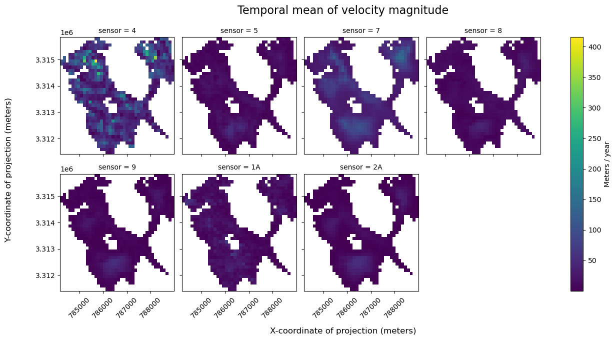
It’s important to keep in mind that in addition to having different spectral properties and imaging resolutions, the sensors included in the ITS_LIVE dataset have been active during different, and sometimes overlapping periods of time. There is additional discussion of inter-sensor bias in the ITS_LIVE Known Issues documentation.
B. Examine velocity variability#
1) Histograms and summary statistics#
First, we plot histogram of the v, vx and vy variables to examine their distrubtions. To construct these plots, we use a combination of xarray plotting functionality and matplotlib object-oriented plotting. In addition, we use xr.reduce() and scipy.stats.skew() to calculate the skew of each variable (inset in each sub-plot).
To make things easier, write a function that calculates and hold summary statistics for each variable in a dictionary:
def calc_summary_stats(ds: xr.Dataset, variable:str):
""" I'm a function that calculates summary statistics for a given data variable and returns them as a dict to be used in a plot"""
skew = ds[f'{variable}'].reduce(func=scipy.stats.skew, nan_policy='omit', dim=['x','y','mid_date']).data
mean = ds[f'{variable}'].mean(dim=['x','y','mid_date'], skipna=True).data
median = ds[f'{variable}'].median(dim=['x','y','mid_date'], skipna=True).data
stats_dict = {'skew':skew, 'mean':mean, 'median':median}
return stats_dict
stats_vy = calc_summary_stats(single_glacier_raster, 'vy')
stats_vx = calc_summary_stats(single_glacier_raster, 'vx')
stats_v = calc_summary_stats(single_glacier_raster, 'v')
fig,axs=plt.subplots(ncols=3, figsize=(20,5))
#VY
hist_y = single_glacier_raster.vy.plot.hist(ax=axs[0], bins=100)
cumulative_y = np.cumsum(hist_y[0])
axs[0].plot(hist_y[1][1:], cumulative_y, color='orange', linestyle='-', alpha=0.5)
# VY stats text
axs[0].text(x=-2000, y=2e6, s=f"Skew: {stats_vy['skew']:.3f}", fontsize=12, color='black')
axs[0].text(x=-2000, y=1.5e6, s=f"Mean: {stats_vy['mean']:.3f}", fontsize=12, color='black')
axs[0].text(x=-2000, y=1e6, s=f"Median: {stats_vy['median']:.3f}", fontsize=12, color='black')
#VX
hist_x = single_glacier_raster.vx.plot.hist(ax=axs[1], bins=100)
cumulative_x = np.cumsum(hist_x[0])
axs[1].plot(hist_x[1][1:], cumulative_x, color='orange', linestyle='-', alpha=0.5)
#VX stats text
axs[1].text(x=-2000, y=2e6, s=f"Skew: {stats_vx['skew']:.3f}", fontsize=12, color='black')
axs[1].text(x=-2000, y=1.5e6, s=f"Mean: {stats_vx['mean']:.3f}", fontsize=12, color='black')
axs[1].text(x=-2000, y=1e6, s=f"Median: {stats_vx['median']:.3f}", fontsize=12, color='black')
#V
hist_v = single_glacier_raster.v.plot.hist(ax=axs[2], bins=100)
cumulative_v = np.cumsum(hist_v[0])
axs[2].plot(hist_v[1][1:], cumulative_v, color='orange', linestyle='-', alpha=0.5)
#V stats text
axs[2].text(x=2000, y=2e6, s=f"Skew: {stats_v['skew']:.3f}", fontsize=12, color='black')
axs[2].text(x=2000, y=1.5e6, s=f"Mean: {stats_v['mean']:.3f}", fontsize=12, color='black')
axs[2].text(x=2000, y=1e6, s=f"Median: {stats_v['median']:.3f}", fontsize=12, color='black')
#Formating and labeling
axs[0].set_title('VY')
axs[1].set_title('VX')
axs[2].set_title('V)')
for i in range(len(axs)):
axs[i].set_xlabel(None)
axs[i].set_ylabel(None)
fig.supylabel('# Observations', x=0.08, fontsize=12)
fig.supxlabel('Meters / year', fontsize=12)
fig.suptitle('Histogram (blue) and cumulative distribution function (orange) of velocity components and magnitude', fontsize=16, y=1.05);
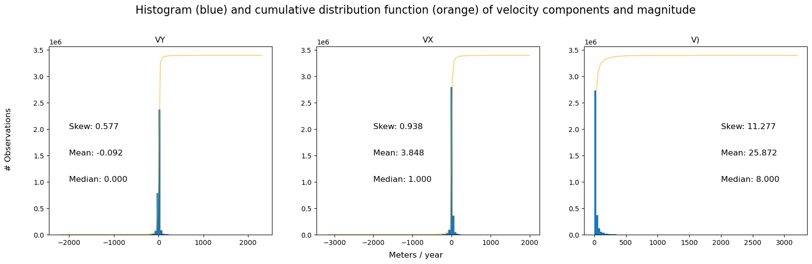
The histograms and summary statistics show that vx and vy distributions are relatively Gaussian, while v is positively skewed and Rician. This is due to the non-linear relationshipp between component and displacement vectors. In datasets such as this one where the signal to noise ratio can be low, calculating velocity magnitude on smoothed or averaged component vectors can help to suppress noise (for a bit more detail, refer to this comment). For this reason, we will usually calculate velocity magnitude after the dataset has been reduced over space or time dimensions.
2) Spatial velocity variability#
Now that we have a greater understanding of the importance of velocity component variability in shaping our understandings of velocity variability, let’s examine these variables as well as the estimated error provided in the dataset by reducing the dataset along the temporal dimension so that we can visualize the data along x and y dimensions.
#Calculate min, max for color bar
vmin_y = single_glacier_raster.vy.mean(dim=['mid_date']).min().data
vmax_y = single_glacier_raster.vy.mean(dim=['mid_date']).max().data
vmin_x = single_glacier_raster.vx.mean(dim=['mid_date']).min().data
vmax_x = single_glacier_raster.vx.mean(dim=['mid_date']).max().data
vmin = min([vmin_x, vmin_y])
vmax = max([vmax_x, vmax_y])
fig, axs = plt.subplots(ncols =2, figsize=(17,7))
x = single_glacier_raster.vx.mean(dim='mid_date').plot(ax=axs[0], vmin=vmin, vmax=vmax, cmap='RdBu_r')
y = single_glacier_raster.vy.mean(dim='mid_date').plot(ax=axs[1], vmin=vmin, vmax=vmax, cmap='RdBu_r')
axs[0].set_title('x-component velocity', fontsize=12)
axs[1].set_title('y-component velocity', fontsize=12)
fig.suptitle('Temporal mean of velocity components', fontsize=16, y=1.02)
x.colorbar.set_label('m/y', rotation=270)
y.colorbar.set_label('m/yr', rotation=270)
for i in range(len(axs)):
axs[i].set_ylabel(None)
axs[i].set_xlabel(None)
fig.supylabel('Y-coordinate of projection (meters)', x=0.08, fontsize=12)
fig.supxlabel('X-coordinate of projection (meters)', fontsize=12);
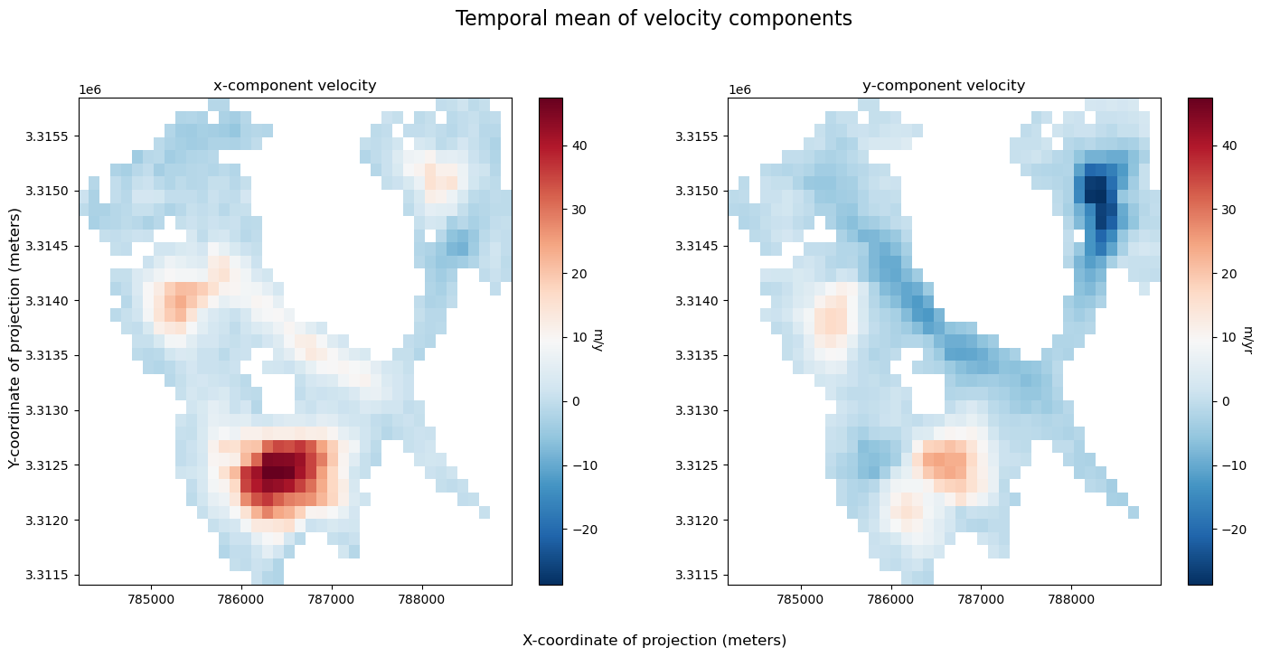
In addition to visualizing components (above), plotting velocity vectors is helpful for understanding magnitude and direction of flow:
First, calculate and visualize mean velocity magnitude over time (we will use the function defined in Part 1), and the mean estimated error over time:
ds_v = calc_v_magnitude(single_glacier_raster.mean(dim='mid_date',skipna=True))
fig, axs= plt.subplots(ncols=2, figsize=(20,7))
single_glacier_vector.plot(ax=axs[0], facecolor='none', edgecolor='red')
single_glacier_raster.mean(dim='mid_date').plot.quiver('x','y','vx','vy', ax=axs[1], angles='xy', robust=True)
single_glacier_vector.plot(ax=axs[1], facecolor='none', edgecolor='red')
a = ds_v['vmag'].plot(ax=axs[0], alpha=0.6, vmax=45, vmin=5)
a.colorbar.set_label('meter/year')
fig.supylabel('Y-coordinate of projection (meters)', x=0.08, fontsize=12)
fig.supxlabel('X-coordinate of projection (meters)', fontsize=12)
fig.suptitle('Velocity vectors (R) and magntiude of velocity (L), averaged over time', fontsize=16, y=0.98)
for i in range(len(axs)):
axs[i].set_xlabel(None)
axs[i].set_ylabel(None)
axs[i].set_title(None);
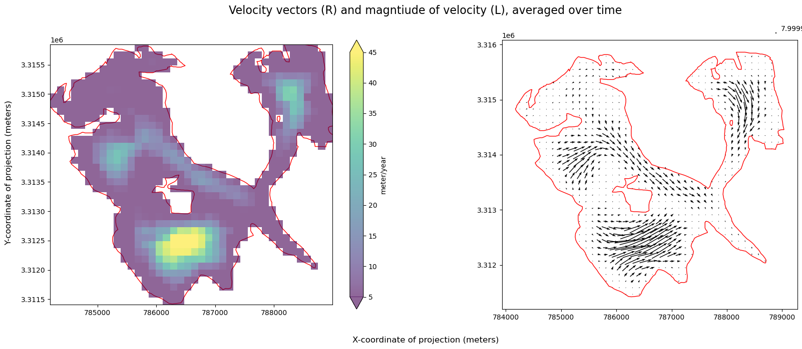
Visualize magnitude of velocity overlaid with velocity vectors next to velocity error:
fig, ax = plt.subplots(figsize=(22,6), ncols=2)
vmag = ds_v.vmag.plot(ax=ax[0], vmin=0, vmax=52,alpha=0.5)
single_glacier_raster.mean(dim='mid_date').plot.quiver('x','y','vx','vy', ax=ax[0], angles='xy', robust=True)
err = ds_v.v_error.plot(ax=ax[1], vmin=0, vmax=52)
vmag.colorbar.set_label('m/y')#, rotation=270)
err.colorbar.set_label('m/y')#, rotation=270)
for i in range(len(ax)):
ax[i].set_ylabel(None)
ax[i].set_xlabel(None)
ax[i].set_title(None)
fig.supxlabel('X-coordinate of projection (meters)', fontsize=12)
fig.supylabel('Y-coordinate of projection (meters)', x=0.08, fontsize=12)
fig.suptitle('Mean velocity magnitude over time (L), mean error over time (R)', fontsize=16, y=1.02);
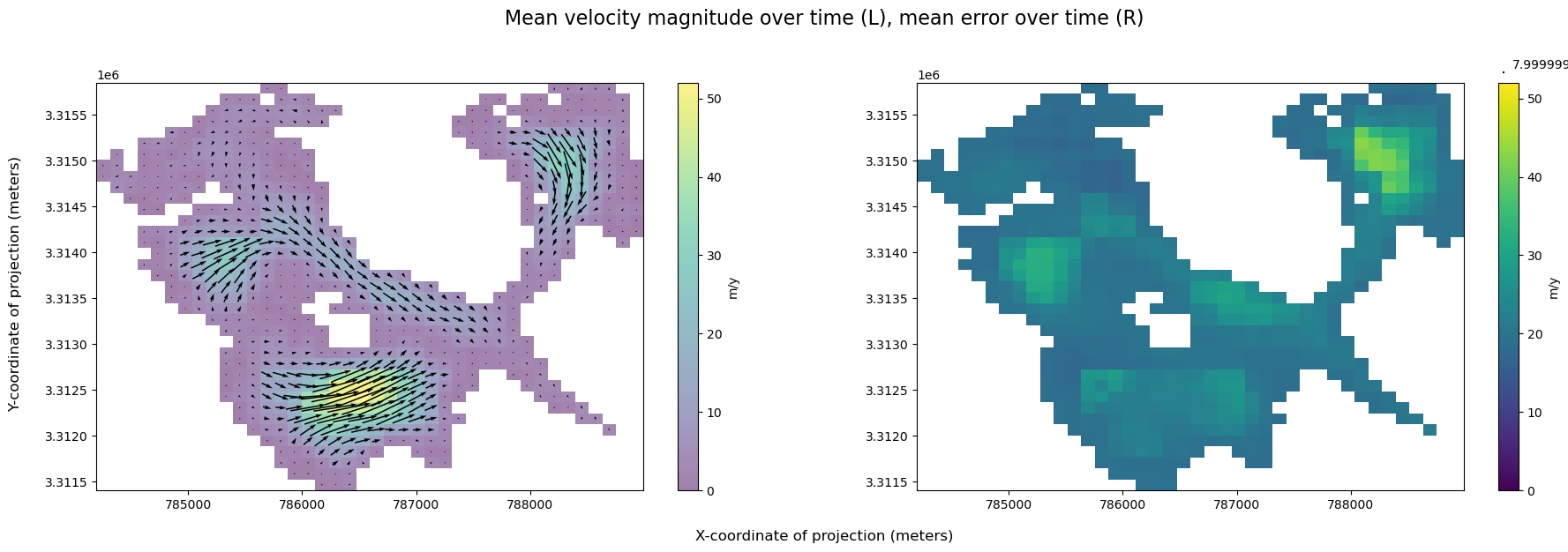
v_error is large relative to the magnitude of velocity, suggesting that this data is pretty noisy.
3) Temporal velocity variability#
Reduce over the spatial dimensions (this time we will switch it up and choose a different reduction function) and visualize variability over time:
fig, ax = plt.subplots(figsize=(20,5))
vmag_med = calc_v_magnitude(single_glacier_raster.median(dim=['x','y']))
vmag_med.plot.scatter(x='mid_date', y='vmag',ax=ax, marker='o', edgecolors='None',alpha=0.5)
fig.suptitle('Spatial median magnitude of velocity over time')
ax.set_title(None)
ax.set_ylabel('m/y')
ax.set_xlabel('Time');
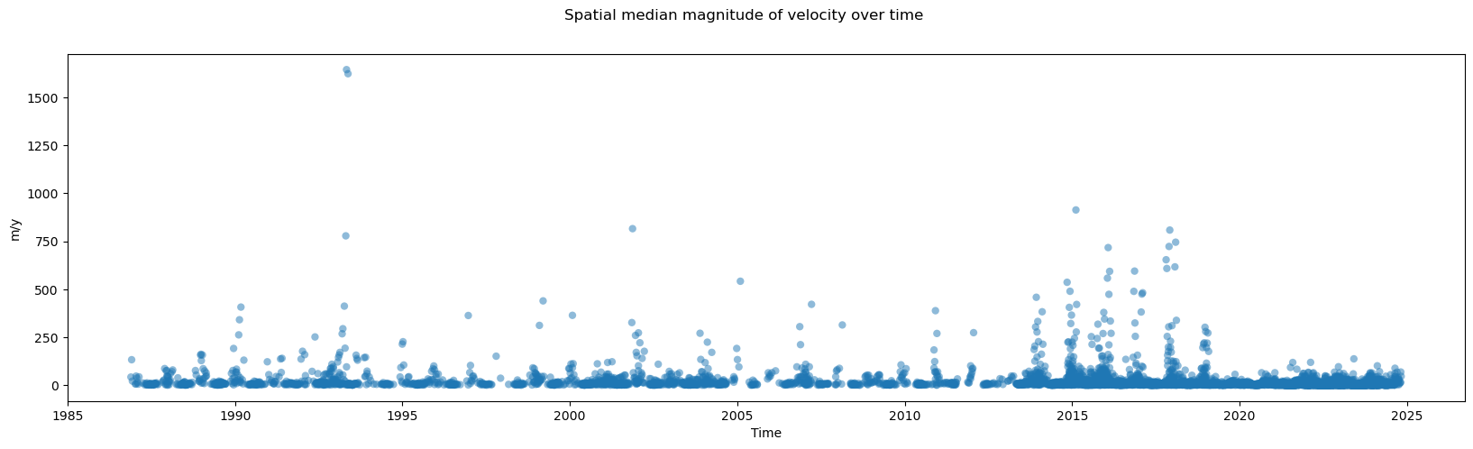
This helps get a sense of velocity variability over time, but also shows how many outliers there are, even after taking the median over the x and y dimensions. In the final section of this notebook, we explore different approaches for changing the resolution of the temporal dimension.
C. Dimensional computations#
In Part 2, we saw that the timeseries is dense in places and quite noisy. This section demonstrates different approaches for looking at a temporal signal in the dataset.
1) Temporal resampling#
Use Xarray’s resample() method to coarsen the dataset. With resample(), you can upsample or downsample the data, choosing both the resample frequency and the type of reduction.
#Coarsen dataset to monthly
resample_obj = single_glacier_raster.resample(mid_date='2ME')
#Calculate monthly median
glacier_resample_1mo = resample_obj.median(dim='mid_date')
The mid_date dimension is now much less dense:
glacier_resample_1mo
<xarray.Dataset> Size: 18MB
Dimensions: (mid_date: 230, y: 37, x: 40)
Coordinates:
mapping int64 8B 0
spatial_ref int64 8B 0
* x (x) float64 320B 7.843e+05 ... 7.889e+05
* y (y) float64 296B 3.316e+06 ... 3.311e+06
* mid_date (mid_date) datetime64[ns] 2kB 1986-09-30 ... ...
Data variables: (12/49)
M11 (mid_date, y, x) float32 1MB nan nan ... nan nan
M11_dr_to_vr_factor (mid_date) float32 920B nan nan nan ... nan nan
M12 (mid_date, y, x) float32 1MB nan nan ... nan nan
M12_dr_to_vr_factor (mid_date) float32 920B nan nan nan ... nan nan
chip_size_height (mid_date, y, x) float32 1MB nan nan ... nan nan
chip_size_width (mid_date, y, x) float32 1MB nan nan ... nan nan
... ...
vy_error_slow (mid_date) float32 920B 30.3 31.4 ... 16.65 26.8
vy_error_stationary (mid_date) float32 920B 30.2 31.45 ... 26.8
vy_stable_shift (mid_date) float32 920B 4.1 -1.0 ... -2.75 71.0
vy_stable_shift_slow (mid_date) float32 920B 4.2 -1.0 ... -2.75 71.0
vy_stable_shift_stationary (mid_date) float32 920B 4.1 -1.0 ... -2.75 71.0
cov (mid_date) float64 2kB 0.0 0.2461 ... 0.0 0.0
Attributes: (12/19)
Conventions: CF-1.8
GDAL_AREA_OR_POINT: Area
author: ITS_LIVE, a NASA MEaSUREs project (its-live.j...
autoRIFT_parameter_file: http://its-live-data.s3.amazonaws.com/autorif...
datacube_software_version: 1.0
date_created: 25-Sep-2023 22:00:23
... ...
s3: s3://its-live-data/datacubes/v2/N30E090/ITS_L...
skipped_granules: s3://its-live-data/datacubes/v2/N30E090/ITS_L...
time_standard_img1: UTC
time_standard_img2: UTC
title: ITS_LIVE datacube of image pair velocities
url: https://its-live-data.s3.amazonaws.com/datacu...- mid_date: 230
- y: 37
- x: 40
- mapping()int640
- crs_wkt :
- PROJCS["WGS 84 / UTM zone 46N",GEOGCS["WGS 84",DATUM["WGS_1984",SPHEROID["WGS 84",6378137,298.257223563]],PRIMEM["Greenwich",0],UNIT["degree",0.0174532925199433,AUTHORITY["EPSG","9122"]],AUTHORITY["EPSG","4326"]],PROJECTION["Transverse_Mercator"],PARAMETER["latitude_of_origin",0],PARAMETER["central_meridian",93],PARAMETER["scale_factor",0.9996],PARAMETER["false_easting",500000],PARAMETER["false_northing",0],UNIT["metre",1],AXIS["Easting",EAST],AXIS["Northing",NORTH],AUTHORITY["EPSG","32646"]]
- semi_major_axis :
- 6378137.0
- semi_minor_axis :
- 6356752.314245179
- inverse_flattening :
- 298.257223563
- reference_ellipsoid_name :
- WGS 84
- longitude_of_prime_meridian :
- 0.0
- prime_meridian_name :
- Greenwich
- geographic_crs_name :
- WGS 84
- horizontal_datum_name :
- World Geodetic System 1984
- projected_crs_name :
- WGS 84 / UTM zone 46N
- grid_mapping_name :
- transverse_mercator
- latitude_of_projection_origin :
- 0.0
- longitude_of_central_meridian :
- 93.0
- false_easting :
- 500000.0
- false_northing :
- 0.0
- scale_factor_at_central_meridian :
- 0.9996
- spatial_ref :
- PROJCS["WGS 84 / UTM zone 46N",GEOGCS["WGS 84",DATUM["WGS_1984",SPHEROID["WGS 84",6378137,298.257223563]],PRIMEM["Greenwich",0],UNIT["degree",0.0174532925199433,AUTHORITY["EPSG","9122"]],AUTHORITY["EPSG","4326"]],PROJECTION["Transverse_Mercator"],PARAMETER["latitude_of_origin",0],PARAMETER["central_meridian",93],PARAMETER["scale_factor",0.9996],PARAMETER["false_easting",500000],PARAMETER["false_northing",0],UNIT["metre",1],AXIS["Easting",EAST],AXIS["Northing",NORTH],AUTHORITY["EPSG","32646"]]
array(0)
- spatial_ref()int640
- GeoTransform :
- 784192.5 120.0 0.0 3315847.5 0.0 -120.0
array(0)
- x(x)float647.843e+05 7.844e+05 ... 7.889e+05
- axis :
- X
- description :
- x coordinate of projection
- long_name :
- x coordinate of projection
- standard_name :
- projection_x_coordinate
- units :
- metre
array([784252.5, 784372.5, 784492.5, 784612.5, 784732.5, 784852.5, 784972.5, 785092.5, 785212.5, 785332.5, 785452.5, 785572.5, 785692.5, 785812.5, 785932.5, 786052.5, 786172.5, 786292.5, 786412.5, 786532.5, 786652.5, 786772.5, 786892.5, 787012.5, 787132.5, 787252.5, 787372.5, 787492.5, 787612.5, 787732.5, 787852.5, 787972.5, 788092.5, 788212.5, 788332.5, 788452.5, 788572.5, 788692.5, 788812.5, 788932.5]) - y(y)float643.316e+06 3.316e+06 ... 3.311e+06
- axis :
- Y
- description :
- y coordinate of projection
- long_name :
- y coordinate of projection
- standard_name :
- projection_y_coordinate
- units :
- metre
array([3315787.5, 3315667.5, 3315547.5, 3315427.5, 3315307.5, 3315187.5, 3315067.5, 3314947.5, 3314827.5, 3314707.5, 3314587.5, 3314467.5, 3314347.5, 3314227.5, 3314107.5, 3313987.5, 3313867.5, 3313747.5, 3313627.5, 3313507.5, 3313387.5, 3313267.5, 3313147.5, 3313027.5, 3312907.5, 3312787.5, 3312667.5, 3312547.5, 3312427.5, 3312307.5, 3312187.5, 3312067.5, 3311947.5, 3311827.5, 3311707.5, 3311587.5, 3311467.5]) - mid_date(mid_date)datetime64[ns]1986-09-30 ... 2024-11-30
- description :
- midpoint of image 1 and image 2 acquisition date and time with granule's centroid longitude and latitude as microseconds
- standard_name :
- image_pair_center_date_with_time_separation
array(['1986-09-30T00:00:00.000000000', '1986-11-30T00:00:00.000000000', '1987-01-31T00:00:00.000000000', ..., '2024-07-31T00:00:00.000000000', '2024-09-30T00:00:00.000000000', '2024-11-30T00:00:00.000000000'], dtype='datetime64[ns]')
- M11(mid_date, y, x)float32nan nan nan nan ... nan nan nan nan
- description :
- conversion matrix element (1st row, 1st column) that can be multiplied with vx to give range pixel displacement dr (see Eq. A18 in https://www.mdpi.com/2072-4292/13/4/749)
- standard_name :
- conversion_matrix_element_11
- units :
- pixel/(meter/year)
array([[[nan, nan, nan, ..., nan, nan, nan], [nan, nan, nan, ..., nan, nan, nan], [nan, nan, nan, ..., nan, nan, nan], ..., [nan, nan, nan, ..., nan, nan, nan], [nan, nan, nan, ..., nan, nan, nan], [nan, nan, nan, ..., nan, nan, nan]], [[nan, nan, nan, ..., nan, nan, nan], [nan, nan, nan, ..., nan, nan, nan], [nan, nan, nan, ..., nan, nan, nan], ..., [nan, nan, nan, ..., nan, nan, nan], [nan, nan, nan, ..., nan, nan, nan], [nan, nan, nan, ..., nan, nan, nan]], [[nan, nan, nan, ..., nan, nan, nan], [nan, nan, nan, ..., nan, nan, nan], [nan, nan, nan, ..., nan, nan, nan], ..., ... ..., [nan, nan, nan, ..., nan, nan, nan], [nan, nan, nan, ..., nan, nan, nan], [nan, nan, nan, ..., nan, nan, nan]], [[nan, nan, nan, ..., nan, nan, nan], [nan, nan, nan, ..., nan, nan, nan], [nan, nan, nan, ..., nan, nan, nan], ..., [nan, nan, nan, ..., nan, nan, nan], [nan, nan, nan, ..., nan, nan, nan], [nan, nan, nan, ..., nan, nan, nan]], [[nan, nan, nan, ..., nan, nan, nan], [nan, nan, nan, ..., nan, nan, nan], [nan, nan, nan, ..., nan, nan, nan], ..., [nan, nan, nan, ..., nan, nan, nan], [nan, nan, nan, ..., nan, nan, nan], [nan, nan, nan, ..., nan, nan, nan]]], dtype=float32) - M11_dr_to_vr_factor(mid_date)float32nan nan nan nan ... nan nan nan nan
- description :
- multiplicative factor that converts slant range pixel displacement dr to slant range velocity vr
- standard_name :
- M11_dr_to_vr_factor
- units :
- meter/(year*pixel)
array([nan, nan, nan, nan, nan, nan, nan, nan, nan, nan, nan, nan, nan, nan, nan, nan, nan, nan, nan, nan, nan, nan, nan, nan, nan, nan, nan, nan, nan, nan, nan, nan, nan, nan, nan, nan, nan, nan, nan, nan, nan, nan, nan, nan, nan, nan, nan, nan, nan, nan, nan, nan, nan, nan, nan, nan, nan, nan, nan, nan, nan, nan, nan, nan, nan, nan, nan, nan, nan, nan, nan, nan, nan, nan, nan, nan, nan, nan, nan, nan, nan, nan, nan, nan, nan, nan, nan, nan, nan, nan, nan, nan, nan, nan, nan, nan, nan, nan, nan, nan, nan, nan, nan, nan, nan, nan, nan, nan, nan, nan, nan, nan, nan, nan, nan, nan, nan, nan, nan, nan, nan, nan, nan, nan, nan, nan, nan, nan, nan, nan, nan, nan, nan, nan, nan, nan, nan, nan, nan, nan, nan, nan, nan, nan, nan, nan, nan, nan, nan, nan, nan, nan, nan, nan, nan, nan, nan, nan, nan, nan, nan, nan, nan, nan, nan, nan, nan, nan, nan, nan, nan, nan, nan, nan, nan, nan, nan, nan, nan, nan, nan, nan, nan, nan, nan, nan, nan, nan, nan, nan, nan, nan, nan, nan, nan, nan, nan, nan, nan, nan, nan, nan, nan, nan, nan, nan, nan, nan, nan, nan, nan, nan, nan, nan, nan, nan, nan, nan, nan, nan, nan, nan, nan, nan, nan, nan, nan, nan, nan, nan], dtype=float32) - M12(mid_date, y, x)float32nan nan nan nan ... nan nan nan nan
- description :
- conversion matrix element (1st row, 2nd column) that can be multiplied with vy to give range pixel displacement dr (see Eq. A18 in https://www.mdpi.com/2072-4292/13/4/749)
- standard_name :
- conversion_matrix_element_12
- units :
- pixel/(meter/year)
array([[[nan, nan, nan, ..., nan, nan, nan], [nan, nan, nan, ..., nan, nan, nan], [nan, nan, nan, ..., nan, nan, nan], ..., [nan, nan, nan, ..., nan, nan, nan], [nan, nan, nan, ..., nan, nan, nan], [nan, nan, nan, ..., nan, nan, nan]], [[nan, nan, nan, ..., nan, nan, nan], [nan, nan, nan, ..., nan, nan, nan], [nan, nan, nan, ..., nan, nan, nan], ..., [nan, nan, nan, ..., nan, nan, nan], [nan, nan, nan, ..., nan, nan, nan], [nan, nan, nan, ..., nan, nan, nan]], [[nan, nan, nan, ..., nan, nan, nan], [nan, nan, nan, ..., nan, nan, nan], [nan, nan, nan, ..., nan, nan, nan], ..., ... ..., [nan, nan, nan, ..., nan, nan, nan], [nan, nan, nan, ..., nan, nan, nan], [nan, nan, nan, ..., nan, nan, nan]], [[nan, nan, nan, ..., nan, nan, nan], [nan, nan, nan, ..., nan, nan, nan], [nan, nan, nan, ..., nan, nan, nan], ..., [nan, nan, nan, ..., nan, nan, nan], [nan, nan, nan, ..., nan, nan, nan], [nan, nan, nan, ..., nan, nan, nan]], [[nan, nan, nan, ..., nan, nan, nan], [nan, nan, nan, ..., nan, nan, nan], [nan, nan, nan, ..., nan, nan, nan], ..., [nan, nan, nan, ..., nan, nan, nan], [nan, nan, nan, ..., nan, nan, nan], [nan, nan, nan, ..., nan, nan, nan]]], dtype=float32) - M12_dr_to_vr_factor(mid_date)float32nan nan nan nan ... nan nan nan nan
- description :
- multiplicative factor that converts slant range pixel displacement dr to slant range velocity vr
- standard_name :
- M12_dr_to_vr_factor
- units :
- meter/(year*pixel)
array([nan, nan, nan, nan, nan, nan, nan, nan, nan, nan, nan, nan, nan, nan, nan, nan, nan, nan, nan, nan, nan, nan, nan, nan, nan, nan, nan, nan, nan, nan, nan, nan, nan, nan, nan, nan, nan, nan, nan, nan, nan, nan, nan, nan, nan, nan, nan, nan, nan, nan, nan, nan, nan, nan, nan, nan, nan, nan, nan, nan, nan, nan, nan, nan, nan, nan, nan, nan, nan, nan, nan, nan, nan, nan, nan, nan, nan, nan, nan, nan, nan, nan, nan, nan, nan, nan, nan, nan, nan, nan, nan, nan, nan, nan, nan, nan, nan, nan, nan, nan, nan, nan, nan, nan, nan, nan, nan, nan, nan, nan, nan, nan, nan, nan, nan, nan, nan, nan, nan, nan, nan, nan, nan, nan, nan, nan, nan, nan, nan, nan, nan, nan, nan, nan, nan, nan, nan, nan, nan, nan, nan, nan, nan, nan, nan, nan, nan, nan, nan, nan, nan, nan, nan, nan, nan, nan, nan, nan, nan, nan, nan, nan, nan, nan, nan, nan, nan, nan, nan, nan, nan, nan, nan, nan, nan, nan, nan, nan, nan, nan, nan, nan, nan, nan, nan, nan, nan, nan, nan, nan, nan, nan, nan, nan, nan, nan, nan, nan, nan, nan, nan, nan, nan, nan, nan, nan, nan, nan, nan, nan, nan, nan, nan, nan, nan, nan, nan, nan, nan, nan, nan, nan, nan, nan, nan, nan, nan, nan, nan, nan], dtype=float32) - chip_size_height(mid_date, y, x)float32nan nan nan nan ... nan nan nan nan
- chip_size_coordinates :
- Optical data: chip_size_coordinates = 'image projection geometry: width = x, height = y'. Radar data: chip_size_coordinates = 'radar geometry: width = range, height = azimuth'
- description :
- height of search template (chip)
- standard_name :
- chip_size_height
- units :
- m
- y_pixel_size :
- 10.0
array([[[ nan, nan, nan, ..., nan, nan, nan], [ nan, nan, nan, ..., nan, nan, nan], [ nan, nan, nan, ..., nan, nan, nan], ..., [ nan, nan, nan, ..., nan, nan, nan], [ nan, nan, nan, ..., nan, nan, nan], [ nan, nan, nan, ..., nan, nan, nan]], [[ nan, nan, nan, ..., 480., nan, nan], [ nan, nan, nan, ..., 480., 480., nan], [ nan, nan, nan, ..., 480., 480., nan], ..., [ nan, nan, nan, ..., nan, nan, nan], [ nan, nan, nan, ..., nan, nan, nan], [ nan, nan, nan, ..., nan, nan, nan]], [[ nan, nan, nan, ..., 480., nan, nan], [ nan, nan, nan, ..., 480., 480., nan], [ nan, nan, nan, ..., 480., 480., nan], ..., ... ..., [ nan, nan, nan, ..., nan, nan, nan], [ nan, nan, nan, ..., nan, nan, nan], [ nan, nan, nan, ..., nan, nan, nan]], [[ nan, nan, nan, ..., 240., nan, nan], [ nan, nan, nan, ..., 240., 240., nan], [ nan, nan, nan, ..., 480., 360., nan], ..., [ nan, nan, nan, ..., nan, nan, nan], [ nan, nan, nan, ..., nan, nan, nan], [ nan, nan, nan, ..., nan, nan, nan]], [[ nan, nan, nan, ..., 360., nan, nan], [ nan, nan, nan, ..., 360., 480., nan], [ nan, nan, nan, ..., 360., 240., nan], ..., [ nan, nan, nan, ..., nan, nan, nan], [ nan, nan, nan, ..., nan, nan, nan], [ nan, nan, nan, ..., nan, nan, nan]]], dtype=float32) - chip_size_width(mid_date, y, x)float32nan nan nan nan ... nan nan nan nan
- chip_size_coordinates :
- Optical data: chip_size_coordinates = 'image projection geometry: width = x, height = y'. Radar data: chip_size_coordinates = 'radar geometry: width = range, height = azimuth'
- description :
- width of search template (chip)
- standard_name :
- chip_size_width
- units :
- m
- x_pixel_size :
- 10.0
array([[[ nan, nan, nan, ..., nan, nan, nan], [ nan, nan, nan, ..., nan, nan, nan], [ nan, nan, nan, ..., nan, nan, nan], ..., [ nan, nan, nan, ..., nan, nan, nan], [ nan, nan, nan, ..., nan, nan, nan], [ nan, nan, nan, ..., nan, nan, nan]], [[ nan, nan, nan, ..., 480., nan, nan], [ nan, nan, nan, ..., 480., 480., nan], [ nan, nan, nan, ..., 480., 480., nan], ..., [ nan, nan, nan, ..., nan, nan, nan], [ nan, nan, nan, ..., nan, nan, nan], [ nan, nan, nan, ..., nan, nan, nan]], [[ nan, nan, nan, ..., 480., nan, nan], [ nan, nan, nan, ..., 480., 480., nan], [ nan, nan, nan, ..., 480., 480., nan], ..., ... ..., [ nan, nan, nan, ..., nan, nan, nan], [ nan, nan, nan, ..., nan, nan, nan], [ nan, nan, nan, ..., nan, nan, nan]], [[ nan, nan, nan, ..., 240., nan, nan], [ nan, nan, nan, ..., 240., 240., nan], [ nan, nan, nan, ..., 480., 360., nan], ..., [ nan, nan, nan, ..., nan, nan, nan], [ nan, nan, nan, ..., nan, nan, nan], [ nan, nan, nan, ..., nan, nan, nan]], [[ nan, nan, nan, ..., 360., nan, nan], [ nan, nan, nan, ..., 360., 480., nan], [ nan, nan, nan, ..., 360., 240., nan], ..., [ nan, nan, nan, ..., nan, nan, nan], [ nan, nan, nan, ..., nan, nan, nan], [ nan, nan, nan, ..., nan, nan, nan]]], dtype=float32) - date_dt(mid_date)timedelta64[ns]95 days 23:56:41.586914063 ... 2...
- description :
- time separation between acquisition of image 1 and image 2
- standard_name :
- image_pair_time_separation
array([ 8294201586914063, 8294282995605472, 11059417529296873, 8294605004882810, 31104539208984378, 31104568212890625, 26266021875000000, 18662643566894531, 5529664599609378, 8985669873046873, 23500955566406252, 33177702832031252, 27648005273437495, 13823964404296878, 4838378082275387, 4147170336914063, 35941999218750000, 27647620312500000, 33177043652343747, 4838311669921877, 5529486456298824, 4147106726074216, 29030133691406252, 34559791699218747, 33177613183593747, 34560125244140625, 5529687011718747, 12441770068359378, 8294498876953121, 30413050488281252, 28339367431640625, 30412876464843747, 12441590771484378, 12441559130859378, 15206311669921873, 27647807519531247, 31103866845703126, 22809513647460936, 10368040209960936, 11059251416015621, 31104046142578121, 26265615820312504, 19353563085937500, 22118267669677734, 8985536389160157, 22118164013671873, 33177129345703121, 34559459472656252, 40088818212890625, 15206082275390621, 2764738119506837, 13823634814453126, 23500130273437495, 30412135546875000, 27647623608398441, 13823824658203126, 5529864660644531, 12442176123046873, 34561352636718747, 33178906494140625, ... 10713597363281252, 24883240869140625, 29721676464843747, 25574550292968747, 13824059985351562, 9676875805664063, 24192065917968747, 29030413183593747, 29030473828125000, 29721721289062504, 15206364404296873, 14169496508789062, 19353590771484378, 31795196044921878, 29030397363281252, 24191857617187495, 12096349365234378, 9676720898437499, 17279720507812499, 25055770605468747, 26265258544921873, 15897439160156252, 12268887670898441, 27648010546875000, 32400007910156247, 30239939355468747, 7775990112304684, 9504000000000000, 6480257739257810, 31320006591796873, 32399997363281252, 32184038232421878, 31536002636718747, 7343988134765621, 8640369799804684, 19008000000000000, 27215997363281252, 34128092285156252, 32832000000000000, 23328319042968747, 18576010546874999, 12528131835937495, 20606232568359378, 26351712597656252, 27648010546875000, 26784210937499999, 16416329589843747, 14255771923828126, 18359759399414062, 29375910351562504, 30671997363281252, 25488226757812504, 20304287402343747, 12095730395507815, 14687690185546873, 20303632177734378, 12960000000000000, 4751998022460936, 2160098052978513], dtype='timedelta64[ns]') - floatingice(mid_date, y, x)float32nan nan nan nan ... nan nan nan nan
- description :
- floating ice mask, 0 = non-floating-ice, 1 = floating-ice
- flag_meanings :
- non-ice ice
- flag_values :
- [0, 1]
- standard_name :
- floating ice mask
- url :
- https://its-live-data.s3.amazonaws.com/autorift_parameters/v001/N46_0120m_floatingice.tif
array([[[nan, nan, nan, ..., 0., nan, nan], [nan, nan, nan, ..., 0., 0., nan], [nan, nan, nan, ..., 0., 0., nan], ..., [nan, nan, nan, ..., nan, nan, nan], [nan, nan, nan, ..., nan, nan, nan], [nan, nan, nan, ..., nan, nan, nan]], [[nan, nan, nan, ..., 0., nan, nan], [nan, nan, nan, ..., 0., 0., nan], [nan, nan, nan, ..., 0., 0., nan], ..., [nan, nan, nan, ..., nan, nan, nan], [nan, nan, nan, ..., nan, nan, nan], [nan, nan, nan, ..., nan, nan, nan]], [[nan, nan, nan, ..., 0., nan, nan], [nan, nan, nan, ..., 0., 0., nan], [nan, nan, nan, ..., 0., 0., nan], ..., ... ..., [nan, nan, nan, ..., nan, nan, nan], [nan, nan, nan, ..., nan, nan, nan], [nan, nan, nan, ..., nan, nan, nan]], [[nan, nan, nan, ..., 0., nan, nan], [nan, nan, nan, ..., 0., 0., nan], [nan, nan, nan, ..., 0., 0., nan], ..., [nan, nan, nan, ..., nan, nan, nan], [nan, nan, nan, ..., nan, nan, nan], [nan, nan, nan, ..., nan, nan, nan]], [[nan, nan, nan, ..., 0., nan, nan], [nan, nan, nan, ..., 0., 0., nan], [nan, nan, nan, ..., 0., 0., nan], ..., [nan, nan, nan, ..., nan, nan, nan], [nan, nan, nan, ..., nan, nan, nan], [nan, nan, nan, ..., nan, nan, nan]]], dtype=float32) - interp_mask(mid_date, y, x)float32nan nan nan nan ... nan nan nan nan
- description :
- light interpolation mask
- flag_meanings :
- measured interpolated
- flag_values :
- [0, 1]
- standard_name :
- interpolated_value_mask
array([[[nan, nan, nan, ..., nan, nan, nan], [nan, nan, nan, ..., nan, nan, nan], [nan, nan, nan, ..., nan, nan, nan], ..., [nan, nan, nan, ..., nan, nan, nan], [nan, nan, nan, ..., nan, nan, nan], [nan, nan, nan, ..., nan, nan, nan]], [[nan, nan, nan, ..., 1., nan, nan], [nan, nan, nan, ..., 1., 1., nan], [nan, nan, nan, ..., 1., 1., nan], ..., [nan, nan, nan, ..., nan, nan, nan], [nan, nan, nan, ..., nan, nan, nan], [nan, nan, nan, ..., nan, nan, nan]], [[nan, nan, nan, ..., nan, nan, nan], [nan, nan, nan, ..., nan, nan, nan], [nan, nan, nan, ..., 1., nan, nan], ..., ... ..., [nan, nan, nan, ..., nan, nan, nan], [nan, nan, nan, ..., nan, nan, nan], [nan, nan, nan, ..., nan, nan, nan]], [[nan, nan, nan, ..., 1., nan, nan], [nan, nan, nan, ..., 1., nan, nan], [nan, nan, nan, ..., 1., 1., nan], ..., [nan, nan, nan, ..., nan, nan, nan], [nan, nan, nan, ..., nan, nan, nan], [nan, nan, nan, ..., nan, nan, nan]], [[nan, nan, nan, ..., 1., nan, nan], [nan, nan, nan, ..., nan, nan, nan], [nan, nan, nan, ..., 1., nan, nan], ..., [nan, nan, nan, ..., nan, nan, nan], [nan, nan, nan, ..., nan, nan, nan], [nan, nan, nan, ..., nan, nan, nan]]], dtype=float32) - landice(mid_date, y, x)float32nan nan nan nan ... nan nan nan nan
- description :
- land ice mask, 0 = non-land-ice, 1 = land-ice
- flag_meanings :
- non-ice ice
- flag_values :
- [0, 1]
- standard_name :
- land ice mask
- url :
- https://its-live-data.s3.amazonaws.com/autorift_parameters/v001/N46_0120m_landice.tif
array([[[nan, nan, nan, ..., 1., nan, nan], [nan, nan, nan, ..., 1., 1., nan], [nan, nan, nan, ..., 1., 1., nan], ..., [nan, nan, nan, ..., nan, nan, nan], [nan, nan, nan, ..., nan, nan, nan], [nan, nan, nan, ..., nan, nan, nan]], [[nan, nan, nan, ..., 1., nan, nan], [nan, nan, nan, ..., 1., 1., nan], [nan, nan, nan, ..., 1., 1., nan], ..., [nan, nan, nan, ..., nan, nan, nan], [nan, nan, nan, ..., nan, nan, nan], [nan, nan, nan, ..., nan, nan, nan]], [[nan, nan, nan, ..., 1., nan, nan], [nan, nan, nan, ..., 1., 1., nan], [nan, nan, nan, ..., 1., 1., nan], ..., ... ..., [nan, nan, nan, ..., nan, nan, nan], [nan, nan, nan, ..., nan, nan, nan], [nan, nan, nan, ..., nan, nan, nan]], [[nan, nan, nan, ..., 1., nan, nan], [nan, nan, nan, ..., 1., 1., nan], [nan, nan, nan, ..., 1., 1., nan], ..., [nan, nan, nan, ..., nan, nan, nan], [nan, nan, nan, ..., nan, nan, nan], [nan, nan, nan, ..., nan, nan, nan]], [[nan, nan, nan, ..., 1., nan, nan], [nan, nan, nan, ..., 1., 1., nan], [nan, nan, nan, ..., 1., 1., nan], ..., [nan, nan, nan, ..., nan, nan, nan], [nan, nan, nan, ..., nan, nan, nan], [nan, nan, nan, ..., nan, nan, nan]]], dtype=float32) - roi_valid_percentage(mid_date)float3216.2 25.0 31.7 ... 32.2 39.65 45.4
- description :
- percentage of pixels with a valid velocity estimate determined for the intersection of the full image pair footprint and the region of interest (roi) that defines where autoRIFT tried to estimate a velocity
- standard_name :
- region_of_interest_valid_pixel_percentage
array([16.2 , 25. , 31.7 , 25. , 24.85 , 37.2 , 44.7 , 28.05 , 79.2 , 13.55 , 28.1 , 39.1 , 25.5 , 15.6 , 36.95 , 22.7 , 18.3 , 37.1 , 36.8 , 28.1 , 49.9 , 41.4 , 20.5 , 44.3 , 33.9 , 28.5 , 27.4 , 35.5 , 30.050001, 29.8 , 26.900002, 27. , 20. , 17.8 , 19.7 , 40.9 , 27.1 , 26.1 , 35.5 , 42.3 , 35.4 , 49.2 , 45.1 , 36.5 , 56.3 , 30.9 , 61.55 , 58.6 , 44.699997, 25.3 , 51.15 , 35.5 , 28.8 , 52.8 , 29.05 , 20.8 , 46.5 , 21. , 17.3 , 39.05 , 28.05 , 14.55 , 29. , 33.7 , 16.4 , 26.2 , 20.2 , 16.800001, 15.9 , 14.7 , 19.1 , 27.55 , 21.400002, 26.8 , 47.15 , 32.300003, 19.2 , 45.9 , 39.4 , 9.65 , 40.5 , 26.2 , 32.2 , 48.7 , 37.5 , 30.5 , 50.1 , 34.3 , 30.2 , 42.6 , 32.5 , 27.55 , 34.8 , 29.3 , 28.1 , 44.9 , 31. , 29.8 , 59.4 , 42.6 , 28.15 , 54.25 , 36.95 , 37.95 , 39.9 , 37.9 , 27.3 , 33.35 , 28.85 , 20.7 , 25.6 , 22.3 , 26. , 32.9 , 25.75 , 19.95 , 27.2 , 13.9 , 22.7 , 37.9 , 24.9 , 22.1 , 39.5 , 27.9 , 15.1 , 36. , 26.6 , 12. , 33. , 16.7 , 18.25 , 61.9 , 20.8 , 27.3 , 79.85 , 28.9 , 28.6 , 52.45 , 26.2 , 32.6 , 31.5 , 25.4 , 35.15 , 37.8 , 30.2 , 43.050003, 50.3 , 35.45 , 27. , 46.949997, 32.95 , 24.55 , 24.3 , 19.85 , 16.4 , 25. , 21. , 14.55 , 28.75 , 23.2 , 19.5 , 34.4 , 37.8 , 48.2 , 48.6 , 33.5 , 44.7 , 52.4 , 41.8 , 29.7 , 48.1 , 42.8 , 45.4 , 46.2 , 45.2 , 42.25 , 40.9 , 35.85 , 36.55 , 41.7 , 32.3 , 27.3 , 34.45 , 32.2 , 27.6 , 51.4 , 30.7 , 32.1 , 44.65 , 35.6 , 40.7 , 49.5 , 37.3 , 37.15 , 39.9 , 40.15 , 45.2 , 45.199997, 41.1 , 52.7 , 43.75 , 49.5 , 57.6 , 67.4 , 58.9 , 61.3 , 47.85 , 46. , 52.7 , 64. , 49.4 , 37.5 , 45. , 40. , 42. , 58. , 48.95 , 36.7 , 44.55 , 40.1 , 38.8 , 57.7 , 48.4 , 36.5 , 46.9 , 47.2 , 38.3 , 32.2 , 39.65 , 45.4 ], dtype=float32) - stable_count_slow(mid_date)float645.932e+04 1.502e+04 ... 3.633e+04
- description :
- number of valid pixels over slowest 25% of ice
- standard_name :
- stable_count_slow
- units :
- count
array([59322. , 15021. , 24305. , 20905. , 23144.5, 33070.5, 32353. , 24972.5, 42573. , 30865.5, 41023. , 35462. , 39650. , 41030.5, 29982.5, 43779. , 42674. , 34729. , 35099. , 53453.5, 38065. , 47672. , 32069. , 30922. , 25455. , 26449. , 14152. , 28025. , 44664. , 37109. , 30579.5, 33417. , 27180. , 42252. , 28111. , 21551. , 37219. , 24239.5, 22551.5, 39914. , 33687. , 38254. , 22153. , 26377. , 18254.5, 53153. , 37647. , 30057. , 23181. , 41130. , 32372.5, 27434. , 42052. , 46846. , 28655.5, 33914. , 28223.5, 40350. , 30472. , 33362.5, 47668.5, 41438.5, 25816. , 15592.5, 46021. , 44671. , 24300. , 37192. , 44169. , 30152. , 23707. , 35336. , 22722.5, 30530. , 34209.5, 45046. , 35811. , 29104. , 46721. , 31303. , 18500.5, 35951. , 32455. , 33184. , 32074. , 25976. , 23207.5, 33269. , 39866. , 34696. , 24618.5, 46908.5, 34647. , 33985. , 36006. , 34751. , 20128. , 39368. , 20469. , 27604. , 28283.5, 27909. , 42142.5, 30684.5, 36587. , 31332. , 17473. , 28493. , 32617. , 43538. , 37609. , 29135. , 30727. , 27793. , 35722.5, 37130.5, 35622. , 36692. , 32534.5, 36063. , 24386. , 33969. , 31448. , 34814. , 29047.5, 28409. , 40649. , 40982. , 35297.5, 33086. , 33680.5, 32189. , 33600. , 30693.5, 42328. , 23049. , 33243. , 32330.5, 32201. , 34781. , 27134. , 36360. , 25191. , 35551.5, 26408.5, 39970. , 24507. , 37154.5, 24761. , 32289.5, 32946. , 37203. , 29296. , 38639. , 36921. , 31426. , 36837. , 35108.5, 35092.5, 42707. , 26455. , 30941. , 22543. , 38742. , 30058. , 35209.5, 30084. , 33232. , 34237. , 33479. , 29456. , 34197.5, 30379. , 30622. , 30960. , 33439. , 35045. , 38729. , 32325. , 32570. , 30505. , 34872. , 29548. , 35044. , 33072. , 31713. , 31601. , 29976. , 33233. , 32373.5, 35625. , 33940.5, 32135. , 35884. , 28092. , 30387. , 36883. , 36182.5, 33042. , 34535. , 33988.5, 32214. , 33215.5, 34789. , 29151. , 29182. , 32458.5, 32800.5, 31893. , 31563. , 32394. , 31920.5, 34549. , 31355. , 32419. , 32403. , 32863. , 32185. , 33031.5, 33439.5, 32636. , 31626. , 32585.5, 30843. , 32779. , 32408. , 31409. , 30384.5, 33028. , 36329. ]) - stable_count_stationary(mid_date)float645.727e+04 1.213e+04 ... 3.519e+04
- description :
- number of valid pixels over stationary or slow-flowing surfaces
- standard_name :
- stable_count_stationary
- units :
- count
array([57272. , 12134.5, 28755. , 31083. , 20664. , 28968.5, 31070. , 24218.5, 33026. , 31171.5, 38542. , 34821. , 33640. , 40427. , 24978.5, 33126. , 42195. , 33520. , 39460. , 51807. , 30219. , 45565. , 29679. , 28256. , 37927. , 21862. , 30112. , 28761. , 41746. , 39341. , 35560. , 33120. , 26658. , 39855. , 26156. , 28870.5, 34196. , 32797.5, 24661. , 35932. , 37782.5, 28717. , 23629.5, 44556. , 21539. , 49669. , 47823.5, 25610. , 52290.5, 38271. , 24269.5, 26798. , 42390. , 39756. , 19486. , 31435. , 48847.5, 32976. , 31719. , 29278. , 53135.5, 40345.5, 27571. , 9001. , 39386. , 44787. , 30763. , 35317. , 42683. , 47592. , 26900. , 38543. , 20191. , 29269. , 33153.5, 37234.5, 35282. , 30915. , 39017.5, 29552. , 24464.5, 34570. , 31018. , 32189. , 30210. , 24342. , 23990. , 28226. , 39553. , 43780.5, 34104. , 45257.5, 33368. , 33127. , 32390. , 38111. , 37777. , 35082.5, 16350. , 26415. , 23190. , 45528.5, 41639. , 40530. , 41340.5, 41035.5, 23224. , 26892. , 34414.5, 41628. , 36321. , 26691. , 35497. , 29912. , 29992.5, 31256. , 29859. , 40906. , 30530. , 35704. , 30100. , 35003. , 33401. , 32026. , 24552.5, 26089. , 39664.5, 41338. , 30833. , 31624. , 31670.5, 33360. , 34646. , 36482. , 36147. , 31700. , 29410. , 31662.5, 29461. , 28753. , 22256. , 33588. , 32202.5, 34964.5, 23724.5, 34225. , 35938. , 33173.5, 26200. , 34635.5, 32515. , 34426.5, 25119.5, 35954. , 38344. , 30710. , 35147. , 33165. , 33317. , 39804. , 26310. , 32117. , 31698. , 36723. , 27614. , 36390.5, 29528. , 34345. , 32715. , 34722. , 30585. , 33173. , 31080.5, 32235. , 31692. , 31758.5, 35398. , 38304.5, 33427.5, 32391. , 31315. , 32988. , 28760. , 32653. , 34326.5, 28694. , 30534. , 31610. , 32061.5, 31826. , 35376. , 32770.5, 32281. , 35631. , 30962. , 30281.5, 36868. , 34895. , 31606. , 35552. , 33086.5, 32534. , 32964. , 32818. , 30358. , 31060. , 31820.5, 32244.5, 31741. , 31757. , 32403. , 31844.5, 34471.5, 31395.5, 31903. , 32493. , 32686.5, 32253. , 32666. , 33650. , 32201. , 32596. , 33226.5, 30354. , 32416.5, 31840.5, 32050. , 30369.5, 32823.5, 35190. ]) - stable_shift_flag(mid_date)float641.0 1.0 1.0 1.0 ... 1.0 1.0 1.0 1.0
- description :
- flag for applying velocity bias correction: 0 = no correction; 1 = correction from overlapping stable surface mask (stationary or slow-flowing surfaces with velocity < 15 m/yr)(top priority); 2 = correction from slowest 25% of overlapping velocities (second priority)
- standard_name :
- stable_shift_flag
array([1., 1., 1., 1., 1., 1., 1., 1., 1., 1., 1., 1., 1., 1., 1., 1., 1., 1., 1., 1., 1., 1., 1., 1., 1., 1., 1., 1., 1., 1., 1., 1., 1., 1., 1., 1., 1., 1., 1., 1., 1., 1., 1., 1., 1., 1., 1., 1., 1., 1., 1., 1., 1., 1., 1., 1., 1., 1., 1., 1., 1., 1., 1., 1., 1., 1., 1., 1., 1., 1., 1., 1., 1., 1., 1., 1., 1., 1., 1., 1., 1., 1., 1., 1., 1., 1., 1., 1., 1., 1., 1., 1., 1., 1., 1., 1., 1., 1., 1., 1., 1., 1., 1., 1., 1., 1., 1., 1., 1., 1., 1., 1., 1., 1., 1., 1., 1., 1., 1., 1., 1., 1., 1., 1., 1., 1., 1., 1., 1., 1., 1., 1., 1., 1., 1., 1., 1., 1., 1., 1., 1., 1., 1., 1., 1., 1., 1., 1., 1., 1., 1., 1., 1., 1., 1., 1., 1., 1., 1., 1., 1., 1., 1., 1., 1., 1., 1., 1., 1., 1., 1., 1., 1., 1., 1., 1., 1., 1., 1., 1., 1., 1., 1., 1., 1., 1., 1., 1., 1., 1., 1., 1., 1., 1., 1., 1., 1., 1., 1., 1., 1., 1., 1., 1., 1., 1., 1., 1., 1., 1., 1., 1., 1., 1., 1., 1., 1., 1., 1., 1., 1., 1., 1., 1., 1., 1., 1., 1., 1., 1.]) - v(mid_date, y, x)float32nan nan nan nan ... nan nan nan nan
- description :
- velocity magnitude
- standard_name :
- land_ice_surface_velocity
- units :
- meter/year
array([[[ nan, nan, nan, ..., nan, nan, nan], [ nan, nan, nan, ..., nan, nan, nan], [ nan, nan, nan, ..., nan, nan, nan], ..., [ nan, nan, nan, ..., nan, nan, nan], [ nan, nan, nan, ..., nan, nan, nan], [ nan, nan, nan, ..., nan, nan, nan]], [[ nan, nan, nan, ..., 178. , nan, nan], [ nan, nan, nan, ..., 164. , 166. , nan], [ nan, nan, nan, ..., 99. , 93. , nan], ..., [ nan, nan, nan, ..., nan, nan, nan], [ nan, nan, nan, ..., nan, nan, nan], [ nan, nan, nan, ..., nan, nan, nan]], [[ nan, nan, nan, ..., 39.5, nan, nan], [ nan, nan, nan, ..., 50.5, 66. , nan], [ nan, nan, nan, ..., 52. , 11. , nan], ..., ... ..., [ nan, nan, nan, ..., nan, nan, nan], [ nan, nan, nan, ..., nan, nan, nan], [ nan, nan, nan, ..., nan, nan, nan]], [[ nan, nan, nan, ..., 26.5, nan, nan], [ nan, nan, nan, ..., 30. , 20. , nan], [ nan, nan, nan, ..., 28. , 18. , nan], ..., [ nan, nan, nan, ..., nan, nan, nan], [ nan, nan, nan, ..., nan, nan, nan], [ nan, nan, nan, ..., nan, nan, nan]], [[ nan, nan, nan, ..., 53.5, nan, nan], [ nan, nan, nan, ..., 25. , 15. , nan], [ nan, nan, nan, ..., 50. , 16. , nan], ..., [ nan, nan, nan, ..., nan, nan, nan], [ nan, nan, nan, ..., nan, nan, nan], [ nan, nan, nan, ..., nan, nan, nan]]], dtype=float32) - v_error(mid_date, y, x)float32nan nan nan nan ... nan nan nan nan
- description :
- velocity magnitude error
- standard_name :
- velocity_error
- units :
- meter/year
array([[[ nan, nan, nan, ..., nan, nan, nan], [ nan, nan, nan, ..., nan, nan, nan], [ nan, nan, nan, ..., nan, nan, nan], ..., [ nan, nan, nan, ..., nan, nan, nan], [ nan, nan, nan, ..., nan, nan, nan], [ nan, nan, nan, ..., nan, nan, nan]], [[ nan, nan, nan, ..., 88. , nan, nan], [ nan, nan, nan, ..., 87. , 86. , nan], [ nan, nan, nan, ..., 72. , 71. , nan], ..., [ nan, nan, nan, ..., nan, nan, nan], [ nan, nan, nan, ..., nan, nan, nan], [ nan, nan, nan, ..., nan, nan, nan]], [[ nan, nan, nan, ..., 24. , nan, nan], [ nan, nan, nan, ..., 23.5, 23. , nan], [ nan, nan, nan, ..., 22. , 22. , nan], ..., ... ..., [ nan, nan, nan, ..., nan, nan, nan], [ nan, nan, nan, ..., nan, nan, nan], [ nan, nan, nan, ..., nan, nan, nan]], [[ nan, nan, nan, ..., 14.5, nan, nan], [ nan, nan, nan, ..., 15. , 15. , nan], [ nan, nan, nan, ..., 16. , 15.5, nan], ..., [ nan, nan, nan, ..., nan, nan, nan], [ nan, nan, nan, ..., nan, nan, nan], [ nan, nan, nan, ..., nan, nan, nan]], [[ nan, nan, nan, ..., 42. , nan, nan], [ nan, nan, nan, ..., 29.5, 24. , nan], [ nan, nan, nan, ..., 34.5, 24. , nan], ..., [ nan, nan, nan, ..., nan, nan, nan], [ nan, nan, nan, ..., nan, nan, nan], [ nan, nan, nan, ..., nan, nan, nan]]], dtype=float32) - va(mid_date, y, x)float32nan nan nan nan ... nan nan nan nan
- description :
- velocity in radar azimuth direction
array([[[nan, nan, nan, ..., nan, nan, nan], [nan, nan, nan, ..., nan, nan, nan], [nan, nan, nan, ..., nan, nan, nan], ..., [nan, nan, nan, ..., nan, nan, nan], [nan, nan, nan, ..., nan, nan, nan], [nan, nan, nan, ..., nan, nan, nan]], [[nan, nan, nan, ..., nan, nan, nan], [nan, nan, nan, ..., nan, nan, nan], [nan, nan, nan, ..., nan, nan, nan], ..., [nan, nan, nan, ..., nan, nan, nan], [nan, nan, nan, ..., nan, nan, nan], [nan, nan, nan, ..., nan, nan, nan]], [[nan, nan, nan, ..., nan, nan, nan], [nan, nan, nan, ..., nan, nan, nan], [nan, nan, nan, ..., nan, nan, nan], ..., ... ..., [nan, nan, nan, ..., nan, nan, nan], [nan, nan, nan, ..., nan, nan, nan], [nan, nan, nan, ..., nan, nan, nan]], [[nan, nan, nan, ..., nan, nan, nan], [nan, nan, nan, ..., nan, nan, nan], [nan, nan, nan, ..., nan, nan, nan], ..., [nan, nan, nan, ..., nan, nan, nan], [nan, nan, nan, ..., nan, nan, nan], [nan, nan, nan, ..., nan, nan, nan]], [[nan, nan, nan, ..., nan, nan, nan], [nan, nan, nan, ..., nan, nan, nan], [nan, nan, nan, ..., nan, nan, nan], ..., [nan, nan, nan, ..., nan, nan, nan], [nan, nan, nan, ..., nan, nan, nan], [nan, nan, nan, ..., nan, nan, nan]]], dtype=float32) - va_error(mid_date)float32nan nan nan nan ... nan nan nan nan
- description :
- error for velocity in radar azimuth direction
- standard_name :
- va_error
- units :
- meter/year
array([ nan, nan, nan, nan, nan, nan, nan, nan, nan, nan, nan, nan, nan, nan, nan, nan, nan, nan, nan, nan, nan, nan, nan, nan, nan, nan, nan, nan, nan, nan, nan, nan, nan, nan, nan, nan, nan, nan, nan, nan, nan, nan, nan, nan, nan, nan, nan, nan, nan, nan, nan, nan, nan, nan, nan, nan, nan, nan, nan, nan, nan, nan, nan, nan, nan, nan, nan, nan, nan, nan, nan, nan, nan, nan, nan, nan, nan, nan, nan, nan, nan, nan, nan, nan, nan, nan, nan, nan, nan, nan, nan, nan, nan, nan, nan, nan, nan, nan, nan, nan, nan, nan, nan, nan, nan, nan, nan, nan, nan, nan, nan, nan, nan, nan, nan, nan, nan, nan, nan, nan, nan, nan, nan, nan, nan, nan, nan, nan, nan, nan, nan, nan, nan, nan, nan, nan, nan, nan, nan, nan, nan, nan, nan, nan, nan, nan, nan, nan, nan, nan, nan, nan, nan, nan, nan, nan, nan, nan, nan, nan, nan, nan, nan, nan, nan, nan, nan, nan, nan, 57.35 , 63. , 71. , 81.85 , 63.5 , nan, nan, nan, nan, nan, nan, nan, nan, nan, 77.3 , 67.45 , 47.4 , 39.85 , 61.3 , 47.25 , 66.850006, 69.4 , 53.3 , 52.7 , 72.45 , 56.6 , 75.6 , 71.850006, 51.85 , 45.15 , 66.5 , 65.1 , 68.05 , 72.899994, 50.1 , 45.1 , 63.7 , 51.4 , 63.5 , 70.3 , 53.35 , 50.85 , 58. , 59.2 , 73.25 , 73.1 , 53.95 , 57.2 , 68.85 , 46.4 , nan, nan, nan, nan, nan, nan, nan, nan, nan, nan, nan], dtype=float32) - va_error_modeled(mid_date)float32nan nan nan nan ... nan nan nan nan
- description :
- 1-sigma error calculated using a modeled error-dt relationship
- standard_name :
- va_error_modeled
- units :
- meter/year
array([ nan, nan, nan, nan, nan, nan, nan, nan, nan, nan, nan, nan, nan, nan, nan, nan, nan, nan, nan, nan, nan, nan, nan, nan, nan, nan, nan, nan, nan, nan, nan, nan, nan, nan, nan, nan, nan, nan, nan, nan, nan, nan, nan, nan, nan, nan, nan, nan, nan, nan, nan, nan, nan, nan, nan, nan, nan, nan, nan, nan, nan, nan, nan, nan, nan, nan, nan, nan, nan, nan, nan, nan, nan, nan, nan, nan, nan, nan, nan, nan, nan, nan, nan, nan, nan, nan, nan, nan, nan, nan, nan, nan, nan, nan, nan, nan, nan, nan, nan, nan, nan, nan, nan, nan, nan, nan, nan, nan, nan, nan, nan, nan, nan, nan, nan, nan, nan, nan, nan, nan, nan, nan, nan, nan, nan, nan, nan, nan, nan, nan, nan, nan, nan, nan, nan, nan, nan, nan, nan, nan, nan, nan, nan, nan, nan, nan, nan, nan, nan, nan, nan, nan, nan, nan, nan, nan, nan, nan, nan, nan, nan, nan, nan, nan, nan, nan, nan, nan, nan, 64.4, 64.4, 64.4, 64.4, 64.4, nan, nan, nan, nan, nan, nan, nan, nan, nan, 64.4, 64.4, 64.4, 64.4, 64.4, 64.4, 64.4, 64.4, 64.4, 64.4, 64.4, 64.4, 64.4, 64.4, 64.4, 64.4, 64.4, 64.4, 64.4, 64.4, 64.4, 64.4, 64.4, 64.4, 64.4, 64.4, 64.4, 64.4, 64.4, 64.4, 64.4, 64.4, 64.4, 64.4, 64.4, 64.4, nan, nan, nan, nan, nan, nan, nan, nan, nan, nan, nan], dtype=float32) - va_error_slow(mid_date)float32nan nan nan nan ... nan nan nan nan
- description :
- RMSE over slowest 25% of retrieved velocities
- standard_name :
- va_error_slow
- units :
- meter/year
array([ nan, nan, nan, nan, nan, nan, nan, nan, nan, nan, nan, nan, nan, nan, nan, nan, nan, nan, nan, nan, nan, nan, nan, nan, nan, nan, nan, nan, nan, nan, nan, nan, nan, nan, nan, nan, nan, nan, nan, nan, nan, nan, nan, nan, nan, nan, nan, nan, nan, nan, nan, nan, nan, nan, nan, nan, nan, nan, nan, nan, nan, nan, nan, nan, nan, nan, nan, nan, nan, nan, nan, nan, nan, nan, nan, nan, nan, nan, nan, nan, nan, nan, nan, nan, nan, nan, nan, nan, nan, nan, nan, nan, nan, nan, nan, nan, nan, nan, nan, nan, nan, nan, nan, nan, nan, nan, nan, nan, nan, nan, nan, nan, nan, nan, nan, nan, nan, nan, nan, nan, nan, nan, nan, nan, nan, nan, nan, nan, nan, nan, nan, nan, nan, nan, nan, nan, nan, nan, nan, nan, nan, nan, nan, nan, nan, nan, nan, nan, nan, nan, nan, nan, nan, nan, nan, nan, nan, nan, nan, nan, nan, nan, nan, nan, nan, nan, nan, nan, nan, 57.35 , 63. , 71. , 81.85 , 63.5 , nan, nan, nan, nan, nan, nan, nan, nan, nan, 77.3 , 67.45 , 47.4 , 39.85 , 61.3 , 47.25 , 66.850006, 69.4 , 53.3 , 52.7 , 72.45 , 56.6 , 75.6 , 71.850006, 51.85 , 45.15 , 66.5 , 65.1 , 68.05 , 72.899994, 50.1 , 45.1 , 63.7 , 51.4 , 63.5 , 70.3 , 53.35 , 50.85 , 58. , 59.2 , 73.25 , 73. , 53.95 , 57.2 , 68.75 , 46.4 , nan, nan, nan, nan, nan, nan, nan, nan, nan, nan, nan], dtype=float32) - va_error_stationary(mid_date)float32nan nan nan nan ... nan nan nan nan
- description :
- RMSE over stable surfaces, stationary or slow-flowing surfaces with velocity < 15 m/yr identified from an external mask
- standard_name :
- va_error_stationary
- units :
- meter/year
array([ nan, nan, nan, nan, nan, nan, nan, nan, nan, nan, nan, nan, nan, nan, nan, nan, nan, nan, nan, nan, nan, nan, nan, nan, nan, nan, nan, nan, nan, nan, nan, nan, nan, nan, nan, nan, nan, nan, nan, nan, nan, nan, nan, nan, nan, nan, nan, nan, nan, nan, nan, nan, nan, nan, nan, nan, nan, nan, nan, nan, nan, nan, nan, nan, nan, nan, nan, nan, nan, nan, nan, nan, nan, nan, nan, nan, nan, nan, nan, nan, nan, nan, nan, nan, nan, nan, nan, nan, nan, nan, nan, nan, nan, nan, nan, nan, nan, nan, nan, nan, nan, nan, nan, nan, nan, nan, nan, nan, nan, nan, nan, nan, nan, nan, nan, nan, nan, nan, nan, nan, nan, nan, nan, nan, nan, nan, nan, nan, nan, nan, nan, nan, nan, nan, nan, nan, nan, nan, nan, nan, nan, nan, nan, nan, nan, nan, nan, nan, nan, nan, nan, nan, nan, nan, nan, nan, nan, nan, nan, nan, nan, nan, nan, nan, nan, nan, nan, nan, nan, 57.35 , 63. , 71. , 81.85 , 63.5 , nan, nan, nan, nan, nan, nan, nan, nan, nan, 77.3 , 67.45 , 47.4 , 39.85 , 61.3 , 47.25 , 66.850006, 69.4 , 53.3 , 52.7 , 72.45 , 56.6 , 75.6 , 71.850006, 51.85 , 45.15 , 66.5 , 65.1 , 68.05 , 72.899994, 50.1 , 45.1 , 63.7 , 51.4 , 63.5 , 70.3 , 53.35 , 50.85 , 58. , 59.2 , 73.25 , 73.1 , 53.95 , 57.2 , 68.85 , 46.4 , nan, nan, nan, nan, nan, nan, nan, nan, nan, nan, nan], dtype=float32) - va_stable_shift(mid_date)float32nan nan nan nan ... nan nan nan nan
- description :
- applied va shift calibrated using pixels over stable or slow surfaces
- standard_name :
- va_stable_shift
- units :
- meter/year
array([ nan, nan, nan, nan, nan, nan, nan, nan, nan, nan, nan, nan, nan, nan, nan, nan, nan, nan, nan, nan, nan, nan, nan, nan, nan, nan, nan, nan, nan, nan, nan, nan, nan, nan, nan, nan, nan, nan, nan, nan, nan, nan, nan, nan, nan, nan, nan, nan, nan, nan, nan, nan, nan, nan, nan, nan, nan, nan, nan, nan, nan, nan, nan, nan, nan, nan, nan, nan, nan, nan, nan, nan, nan, nan, nan, nan, nan, nan, nan, nan, nan, nan, nan, nan, nan, nan, nan, nan, nan, nan, nan, nan, nan, nan, nan, nan, nan, nan, nan, nan, nan, nan, nan, nan, nan, nan, nan, nan, nan, nan, nan, nan, nan, nan, nan, nan, nan, nan, nan, nan, nan, nan, nan, nan, nan, nan, nan, nan, nan, nan, nan, nan, nan, nan, nan, nan, nan, nan, nan, nan, nan, nan, nan, nan, nan, nan, nan, nan, nan, nan, nan, nan, nan, nan, nan, nan, nan, nan, nan, nan, nan, nan, nan, nan, nan, nan, nan, nan, nan, -3.3, 0. , -4.1, 3.3, -7.4, nan, nan, nan, nan, nan, nan, nan, nan, nan, 0. , 0. , 0. , 0. , 0. , 0. , 0. , 0. , 0. , 0. , 0. , 0. , 0. , 0. , 0. , 0. , 0. , 0. , 0. , 0. , 0. , 0. , 0. , 0. , 0. , 0. , 0. , 0. , 0. , 0. , 0. , 0. , 0. , 0. , 0. , 0. , nan, nan, nan, nan, nan, nan, nan, nan, nan, nan, nan], dtype=float32) - va_stable_shift_slow(mid_date)float32nan nan nan nan ... nan nan nan nan
- description :
- va shift calibrated using valid pixels over slowest 25% of retrieved velocities
- standard_name :
- va_stable_shift_slow
- units :
- meter/year
array([ nan, nan, nan, nan, nan, nan, nan, nan, nan, nan, nan, nan, nan, nan, nan, nan, nan, nan, nan, nan, nan, nan, nan, nan, nan, nan, nan, nan, nan, nan, nan, nan, nan, nan, nan, nan, nan, nan, nan, nan, nan, nan, nan, nan, nan, nan, nan, nan, nan, nan, nan, nan, nan, nan, nan, nan, nan, nan, nan, nan, nan, nan, nan, nan, nan, nan, nan, nan, nan, nan, nan, nan, nan, nan, nan, nan, nan, nan, nan, nan, nan, nan, nan, nan, nan, nan, nan, nan, nan, nan, nan, nan, nan, nan, nan, nan, nan, nan, nan, nan, nan, nan, nan, nan, nan, nan, nan, nan, nan, nan, nan, nan, nan, nan, nan, nan, nan, nan, nan, nan, nan, nan, nan, nan, nan, nan, nan, nan, nan, nan, nan, nan, nan, nan, nan, nan, nan, nan, nan, nan, nan, nan, nan, nan, nan, nan, nan, nan, nan, nan, nan, nan, nan, nan, nan, nan, nan, nan, nan, nan, nan, nan, nan, nan, nan, nan, nan, nan, nan, -3.3, 0. , -4.1, 3.3, -7.4, nan, nan, nan, nan, nan, nan, nan, nan, nan, 0. , 0. , 0. , 0. , 0. , 0. , 0. , 0. , 0. , 0. , 0. , 0. , 0. , 0. , 0. , 0. , 0. , 0. , 0. , 0. , 0. , 0. , 0. , 0. , 0. , 0. , 0. , 0. , 0. , 0. , 0. , 0. , 0. , 0. , 0. , 0. , nan, nan, nan, nan, nan, nan, nan, nan, nan, nan, nan], dtype=float32) - va_stable_shift_stationary(mid_date)float32nan nan nan nan ... nan nan nan nan
- description :
- va shift calibrated using valid pixels over stable surfaces, stationary or slow-flowing surfaces with velocity < 15 m/yr identified from an external mask
- standard_name :
- va_stable_shift_stationary
- units :
- meter/year
array([ nan, nan, nan, nan, nan, nan, nan, nan, nan, nan, nan, nan, nan, nan, nan, nan, nan, nan, nan, nan, nan, nan, nan, nan, nan, nan, nan, nan, nan, nan, nan, nan, nan, nan, nan, nan, nan, nan, nan, nan, nan, nan, nan, nan, nan, nan, nan, nan, nan, nan, nan, nan, nan, nan, nan, nan, nan, nan, nan, nan, nan, nan, nan, nan, nan, nan, nan, nan, nan, nan, nan, nan, nan, nan, nan, nan, nan, nan, nan, nan, nan, nan, nan, nan, nan, nan, nan, nan, nan, nan, nan, nan, nan, nan, nan, nan, nan, nan, nan, nan, nan, nan, nan, nan, nan, nan, nan, nan, nan, nan, nan, nan, nan, nan, nan, nan, nan, nan, nan, nan, nan, nan, nan, nan, nan, nan, nan, nan, nan, nan, nan, nan, nan, nan, nan, nan, nan, nan, nan, nan, nan, nan, nan, nan, nan, nan, nan, nan, nan, nan, nan, nan, nan, nan, nan, nan, nan, nan, nan, nan, nan, nan, nan, nan, nan, nan, nan, nan, nan, -3.3, 0. , -4.1, 3.3, -7.4, nan, nan, nan, nan, nan, nan, nan, nan, nan, 0. , 0. , 0. , 0. , 0. , 0. , 0. , 0. , 0. , 0. , 0. , 0. , 0. , 0. , 0. , 0. , 0. , 0. , 0. , 0. , 0. , 0. , 0. , 0. , 0. , 0. , 0. , 0. , 0. , 0. , 0. , 0. , 0. , 0. , 0. , 0. , nan, nan, nan, nan, nan, nan, nan, nan, nan, nan, nan], dtype=float32) - vr(mid_date, y, x)float32nan nan nan nan ... nan nan nan nan
- description :
- velocity in radar range direction
array([[[nan, nan, nan, ..., nan, nan, nan], [nan, nan, nan, ..., nan, nan, nan], [nan, nan, nan, ..., nan, nan, nan], ..., [nan, nan, nan, ..., nan, nan, nan], [nan, nan, nan, ..., nan, nan, nan], [nan, nan, nan, ..., nan, nan, nan]], [[nan, nan, nan, ..., nan, nan, nan], [nan, nan, nan, ..., nan, nan, nan], [nan, nan, nan, ..., nan, nan, nan], ..., [nan, nan, nan, ..., nan, nan, nan], [nan, nan, nan, ..., nan, nan, nan], [nan, nan, nan, ..., nan, nan, nan]], [[nan, nan, nan, ..., nan, nan, nan], [nan, nan, nan, ..., nan, nan, nan], [nan, nan, nan, ..., nan, nan, nan], ..., ... ..., [nan, nan, nan, ..., nan, nan, nan], [nan, nan, nan, ..., nan, nan, nan], [nan, nan, nan, ..., nan, nan, nan]], [[nan, nan, nan, ..., nan, nan, nan], [nan, nan, nan, ..., nan, nan, nan], [nan, nan, nan, ..., nan, nan, nan], ..., [nan, nan, nan, ..., nan, nan, nan], [nan, nan, nan, ..., nan, nan, nan], [nan, nan, nan, ..., nan, nan, nan]], [[nan, nan, nan, ..., nan, nan, nan], [nan, nan, nan, ..., nan, nan, nan], [nan, nan, nan, ..., nan, nan, nan], ..., [nan, nan, nan, ..., nan, nan, nan], [nan, nan, nan, ..., nan, nan, nan], [nan, nan, nan, ..., nan, nan, nan]]], dtype=float32) - vr_error(mid_date)float32nan nan nan nan ... nan nan nan nan
- description :
- error for velocity in radar range direction
- standard_name :
- vr_error
- units :
- meter/year
array([ nan, nan, nan, nan, nan, nan, nan, nan, nan, nan, nan, nan, nan, nan, nan, nan, nan, nan, nan, nan, nan, nan, nan, nan, nan, nan, nan, nan, nan, nan, nan, nan, nan, nan, nan, nan, nan, nan, nan, nan, nan, nan, nan, nan, nan, nan, nan, nan, nan, nan, nan, nan, nan, nan, nan, nan, nan, nan, nan, nan, nan, nan, nan, nan, nan, nan, nan, nan, nan, nan, nan, nan, nan, nan, nan, nan, nan, nan, nan, nan, nan, nan, nan, nan, nan, nan, nan, nan, nan, nan, nan, nan, nan, nan, nan, nan, nan, nan, nan, nan, nan, nan, nan, nan, nan, nan, nan, nan, nan, nan, nan, nan, nan, nan, nan, nan, nan, nan, nan, nan, nan, nan, nan, nan, nan, nan, nan, nan, nan, nan, nan, nan, nan, nan, nan, nan, nan, nan, nan, nan, nan, nan, nan, nan, nan, nan, nan, nan, nan, nan, nan, nan, nan, nan, nan, nan, nan, nan, nan, nan, nan, nan, nan, nan, nan, nan, nan, nan, nan, 17.75 , 19.3 , 22.5 , 27.85 , 19.3 , nan, nan, nan, nan, nan, nan, nan, nan, nan, 25.5 , 18.85 , 12.35 , 8.95 , 15.3 , 12.15 , 20.3 , 20.7 , 14. , 15.1 , 21. , 16.4 , 21.4 , 18.1 , 12.25 , 11.85 , 19.8 , 18.45 , 21.25 , 20.349998, 12.3 , 12.9 , 18.849998, 13.1 , 19.6 , 21.25 , 15. , 14.5 , 17.2 , 17.4 , 22.65 , 21.9 , 14.25 , 14.6 , 18.75 , 11.6 , nan, nan, nan, nan, nan, nan, nan, nan, nan, nan, nan], dtype=float32) - vr_error_modeled(mid_date)float32nan nan nan nan ... nan nan nan nan
- description :
- 1-sigma error calculated using a modeled error-dt relationship
- standard_name :
- vr_error_modeled
- units :
- meter/year
array([ nan, nan, nan, nan, nan, nan, nan, nan, nan, nan, nan, nan, nan, nan, nan, nan, nan, nan, nan, nan, nan, nan, nan, nan, nan, nan, nan, nan, nan, nan, nan, nan, nan, nan, nan, nan, nan, nan, nan, nan, nan, nan, nan, nan, nan, nan, nan, nan, nan, nan, nan, nan, nan, nan, nan, nan, nan, nan, nan, nan, nan, nan, nan, nan, nan, nan, nan, nan, nan, nan, nan, nan, nan, nan, nan, nan, nan, nan, nan, nan, nan, nan, nan, nan, nan, nan, nan, nan, nan, nan, nan, nan, nan, nan, nan, nan, nan, nan, nan, nan, nan, nan, nan, nan, nan, nan, nan, nan, nan, nan, nan, nan, nan, nan, nan, nan, nan, nan, nan, nan, nan, nan, nan, nan, nan, nan, nan, nan, nan, nan, nan, nan, nan, nan, nan, nan, nan, nan, nan, nan, nan, nan, nan, nan, nan, nan, nan, nan, nan, nan, nan, nan, nan, nan, nan, nan, nan, nan, nan, nan, nan, nan, nan, nan, nan, nan, nan, nan, nan, 19.8, 19.8, 19.8, 19.8, 19.8, nan, nan, nan, nan, nan, nan, nan, nan, nan, 19.8, 19.8, 19.8, 19.8, 19.8, 19.8, 19.8, 19.8, 19.8, 19.8, 19.8, 19.8, 19.8, 19.8, 19.8, 19.8, 19.8, 19.8, 19.8, 19.8, 19.8, 19.8, 19.8, 19.8, 19.8, 19.8, 19.8, 19.8, 19.8, 19.8, 19.8, 19.8, 19.8, 19.8, 19.8, 19.8, nan, nan, nan, nan, nan, nan, nan, nan, nan, nan, nan], dtype=float32) - vr_error_slow(mid_date)float32nan nan nan nan ... nan nan nan nan
- description :
- RMSE over slowest 25% of retrieved velocities
- standard_name :
- vr_error_slow
- units :
- meter/year
array([ nan, nan, nan, nan, nan, nan, nan, nan, nan, nan, nan, nan, nan, nan, nan, nan, nan, nan, nan, nan, nan, nan, nan, nan, nan, nan, nan, nan, nan, nan, nan, nan, nan, nan, nan, nan, nan, nan, nan, nan, nan, nan, nan, nan, nan, nan, nan, nan, nan, nan, nan, nan, nan, nan, nan, nan, nan, nan, nan, nan, nan, nan, nan, nan, nan, nan, nan, nan, nan, nan, nan, nan, nan, nan, nan, nan, nan, nan, nan, nan, nan, nan, nan, nan, nan, nan, nan, nan, nan, nan, nan, nan, nan, nan, nan, nan, nan, nan, nan, nan, nan, nan, nan, nan, nan, nan, nan, nan, nan, nan, nan, nan, nan, nan, nan, nan, nan, nan, nan, nan, nan, nan, nan, nan, nan, nan, nan, nan, nan, nan, nan, nan, nan, nan, nan, nan, nan, nan, nan, nan, nan, nan, nan, nan, nan, nan, nan, nan, nan, nan, nan, nan, nan, nan, nan, nan, nan, nan, nan, nan, nan, nan, nan, nan, nan, nan, nan, nan, nan, 17.75 , 19.3 , 22.5 , 27.85 , 19.3 , nan, nan, nan, nan, nan, nan, nan, nan, nan, 25.5 , 18.85 , 12.35 , 8.95 , 15.3 , 12.15 , 20.3 , 20.7 , 14. , 15.1 , 21. , 16.4 , 21.4 , 18.1 , 12.25 , 11.85 , 19.8 , 18.45 , 21.25 , 20.349998, 12.3 , 12.9 , 18.849998, 13.1 , 19.6 , 21.25 , 15. , 14.5 , 17.2 , 17.4 , 22.65 , 21.9 , 14.25 , 14.5 , 18.7 , 11.6 , nan, nan, nan, nan, nan, nan, nan, nan, nan, nan, nan], dtype=float32) - vr_error_stationary(mid_date)float32nan nan nan nan ... nan nan nan nan
- description :
- RMSE over stable surfaces, stationary or slow-flowing surfaces with velocity < 15 m/yr identified from an external mask
- standard_name :
- vr_error_stationary
- units :
- meter/year
array([ nan, nan, nan, nan, nan, nan, nan, nan, nan, nan, nan, nan, nan, nan, nan, nan, nan, nan, nan, nan, nan, nan, nan, nan, nan, nan, nan, nan, nan, nan, nan, nan, nan, nan, nan, nan, nan, nan, nan, nan, nan, nan, nan, nan, nan, nan, nan, nan, nan, nan, nan, nan, nan, nan, nan, nan, nan, nan, nan, nan, nan, nan, nan, nan, nan, nan, nan, nan, nan, nan, nan, nan, nan, nan, nan, nan, nan, nan, nan, nan, nan, nan, nan, nan, nan, nan, nan, nan, nan, nan, nan, nan, nan, nan, nan, nan, nan, nan, nan, nan, nan, nan, nan, nan, nan, nan, nan, nan, nan, nan, nan, nan, nan, nan, nan, nan, nan, nan, nan, nan, nan, nan, nan, nan, nan, nan, nan, nan, nan, nan, nan, nan, nan, nan, nan, nan, nan, nan, nan, nan, nan, nan, nan, nan, nan, nan, nan, nan, nan, nan, nan, nan, nan, nan, nan, nan, nan, nan, nan, nan, nan, nan, nan, nan, nan, nan, nan, nan, nan, 17.75 , 19.3 , 22.5 , 27.85 , 19.3 , nan, nan, nan, nan, nan, nan, nan, nan, nan, 25.5 , 18.85 , 12.35 , 8.95 , 15.3 , 12.15 , 20.3 , 20.7 , 14. , 15.1 , 21. , 16.4 , 21.4 , 18.1 , 12.25 , 11.85 , 19.8 , 18.45 , 21.25 , 20.349998, 12.3 , 12.9 , 18.849998, 13.1 , 19.6 , 21.25 , 15. , 14.5 , 17.2 , 17.4 , 22.65 , 21.9 , 14.25 , 14.6 , 18.75 , 11.6 , nan, nan, nan, nan, nan, nan, nan, nan, nan, nan, nan], dtype=float32) - vr_stable_shift(mid_date)float32nan nan nan nan ... nan nan nan nan
- description :
- applied vr shift calibrated using pixels over stable or slow surfaces
- standard_name :
- vr_stable_shift
- units :
- meter/year
array([ nan, nan, nan, nan, nan, nan, nan, nan, nan, nan, nan, nan, nan, nan, nan, nan, nan, nan, nan, nan, nan, nan, nan, nan, nan, nan, nan, nan, nan, nan, nan, nan, nan, nan, nan, nan, nan, nan, nan, nan, nan, nan, nan, nan, nan, nan, nan, nan, nan, nan, nan, nan, nan, nan, nan, nan, nan, nan, nan, nan, nan, nan, nan, nan, nan, nan, nan, nan, nan, nan, nan, nan, nan, nan, nan, nan, nan, nan, nan, nan, nan, nan, nan, nan, nan, nan, nan, nan, nan, nan, nan, nan, nan, nan, nan, nan, nan, nan, nan, nan, nan, nan, nan, nan, nan, nan, nan, nan, nan, nan, nan, nan, nan, nan, nan, nan, nan, nan, nan, nan, nan, nan, nan, nan, nan, nan, nan, nan, nan, nan, nan, nan, nan, nan, nan, nan, nan, nan, nan, nan, nan, nan, nan, nan, nan, nan, nan, nan, nan, nan, nan, nan, nan, nan, nan, nan, nan, nan, nan, nan, nan, nan, nan, nan, nan, nan, nan, nan, nan, 0. , -2.2 , -2.2 , 2.2 , -0.2 , nan, nan, nan, nan, nan, nan, nan, nan, nan, 0. , -0.2 , 0. , 0. , -0.7 , -0.5 , 0. , 0. , 0. , 0. , 0. , 0. , 0. , 2.1 , 1.1 , -1.05, 0. , 0. , 0. , 1.4 , -1.45, 0. , 0. , 0. , 0. , 0. , 1.85, 0. , 0. , 0. , 0. , 0. , 0. , 0. , -1.85, 2.2 , nan, nan, nan, nan, nan, nan, nan, nan, nan, nan, nan], dtype=float32) - vr_stable_shift_slow(mid_date)float32nan nan nan nan ... nan nan nan nan
- description :
- vr shift calibrated using valid pixels over slowest 25% of retrieved velocities
- standard_name :
- vr_stable_shift_slow
- units :
- meter/year
array([ nan, nan, nan, nan, nan, nan, nan, nan, nan, nan, nan, nan, nan, nan, nan, nan, nan, nan, nan, nan, nan, nan, nan, nan, nan, nan, nan, nan, nan, nan, nan, nan, nan, nan, nan, nan, nan, nan, nan, nan, nan, nan, nan, nan, nan, nan, nan, nan, nan, nan, nan, nan, nan, nan, nan, nan, nan, nan, nan, nan, nan, nan, nan, nan, nan, nan, nan, nan, nan, nan, nan, nan, nan, nan, nan, nan, nan, nan, nan, nan, nan, nan, nan, nan, nan, nan, nan, nan, nan, nan, nan, nan, nan, nan, nan, nan, nan, nan, nan, nan, nan, nan, nan, nan, nan, nan, nan, nan, nan, nan, nan, nan, nan, nan, nan, nan, nan, nan, nan, nan, nan, nan, nan, nan, nan, nan, nan, nan, nan, nan, nan, nan, nan, nan, nan, nan, nan, nan, nan, nan, nan, nan, nan, nan, nan, nan, nan, nan, nan, nan, nan, nan, nan, nan, nan, nan, nan, nan, nan, nan, nan, nan, nan, nan, nan, nan, nan, nan, nan, 0. , -2.2 , -2.2 , 2.2 , -0.2 , nan, nan, nan, nan, nan, nan, nan, nan, nan, 0. , -0.2 , 0. , 0. , -0.7 , -0.5 , 0. , 0. , 0. , 0. , 0. , 0. , 0. , 2.1 , 1.1 , -1.1 , 0. , 0. , 0. , 1.4 , -1.45, 0. , 0. , 0. , 0. , 0. , 1.85, 0. , 0. , 0. , 0. , 0. , 0. , 0. , -1.85, 2.2 , nan, nan, nan, nan, nan, nan, nan, nan, nan, nan, nan], dtype=float32) - vr_stable_shift_stationary(mid_date)float32nan nan nan nan ... nan nan nan nan
- description :
- vr shift calibrated using valid pixels over stable surfaces, stationary or slow-flowing surfaces with velocity < 15 m/yr identified from an external mask
- standard_name :
- vr_stable_shift_stationary
- units :
- meter/year
array([ nan, nan, nan, nan, nan, nan, nan, nan, nan, nan, nan, nan, nan, nan, nan, nan, nan, nan, nan, nan, nan, nan, nan, nan, nan, nan, nan, nan, nan, nan, nan, nan, nan, nan, nan, nan, nan, nan, nan, nan, nan, nan, nan, nan, nan, nan, nan, nan, nan, nan, nan, nan, nan, nan, nan, nan, nan, nan, nan, nan, nan, nan, nan, nan, nan, nan, nan, nan, nan, nan, nan, nan, nan, nan, nan, nan, nan, nan, nan, nan, nan, nan, nan, nan, nan, nan, nan, nan, nan, nan, nan, nan, nan, nan, nan, nan, nan, nan, nan, nan, nan, nan, nan, nan, nan, nan, nan, nan, nan, nan, nan, nan, nan, nan, nan, nan, nan, nan, nan, nan, nan, nan, nan, nan, nan, nan, nan, nan, nan, nan, nan, nan, nan, nan, nan, nan, nan, nan, nan, nan, nan, nan, nan, nan, nan, nan, nan, nan, nan, nan, nan, nan, nan, nan, nan, nan, nan, nan, nan, nan, nan, nan, nan, nan, nan, nan, nan, nan, nan, 0. , -2.2 , -2.2 , 2.2 , -0.2 , nan, nan, nan, nan, nan, nan, nan, nan, nan, 0. , -0.2 , 0. , 0. , -0.7 , -0.5 , 0. , 0. , 0. , 0. , 0. , 0. , 0. , 2.1 , 1.1 , -1.05, 0. , 0. , 0. , 1.4 , -1.45, 0. , 0. , 0. , 0. , 0. , 1.85, 0. , 0. , 0. , 0. , 0. , 0. , 0. , -1.85, 2.2 , nan, nan, nan, nan, nan, nan, nan, nan, nan, nan, nan], dtype=float32) - vx(mid_date, y, x)float32nan nan nan nan ... nan nan nan nan
- description :
- velocity component in x direction
- standard_name :
- land_ice_surface_x_velocity
- units :
- meter/year
array([[[ nan, nan, nan, ..., nan, nan, nan], [ nan, nan, nan, ..., nan, nan, nan], [ nan, nan, nan, ..., nan, nan, nan], ..., [ nan, nan, nan, ..., nan, nan, nan], [ nan, nan, nan, ..., nan, nan, nan], [ nan, nan, nan, ..., nan, nan, nan]], [[ nan, nan, nan, ..., -161. , nan, nan], [ nan, nan, nan, ..., -146. , -143. , nan], [ nan, nan, nan, ..., -90. , -77. , nan], ..., [ nan, nan, nan, ..., nan, nan, nan], [ nan, nan, nan, ..., nan, nan, nan], [ nan, nan, nan, ..., nan, nan, nan]], [[ nan, nan, nan, ..., -30.5, nan, nan], [ nan, nan, nan, ..., -29.5, -28.5, nan], [ nan, nan, nan, ..., -31. , -4. , nan], ..., ... [ nan, nan, nan, ..., nan, nan, nan], [ nan, nan, nan, ..., nan, nan, nan], [ nan, nan, nan, ..., nan, nan, nan]], [[ nan, nan, nan, ..., -10.5, nan, nan], [ nan, nan, nan, ..., -3. , -7. , nan], [ nan, nan, nan, ..., -3. , -3.5, nan], ..., [ nan, nan, nan, ..., nan, nan, nan], [ nan, nan, nan, ..., nan, nan, nan], [ nan, nan, nan, ..., nan, nan, nan]], [[ nan, nan, nan, ..., 13.5, nan, nan], [ nan, nan, nan, ..., 0. , -3. , nan], [ nan, nan, nan, ..., 1. , -15. , nan], ..., [ nan, nan, nan, ..., nan, nan, nan], [ nan, nan, nan, ..., nan, nan, nan], [ nan, nan, nan, ..., nan, nan, nan]]], dtype=float32) - vx_error(mid_date)float3227.4 40.6 24.2 ... 5.6 9.4 17.5
- description :
- best estimate of x_velocity error: vx_error is populated according to the approach used for the velocity bias correction as indicated in "stable_shift_flag"
- standard_name :
- vx_error
- units :
- meter/year
array([ 27.4 , 40.6 , 24.2 , 29.9 , 6.95 , 7.35 , 10.1 , 25.85 , 37.5 , 30.5 , 10.6 , 6.5 , 10. , 19.45 , 54.050003 , 64.4 , 6.7 , 8. , 8. , 47.55 , 39.8 , 51. , 8. , 6.2 , 7.7 , 7.05 , 43.2 , 21.4 , 30.2 , 8.5 , 10.25 , 7.5 , 18. , 19.9 , 20.1 , 9.85 , 10.450001 , 13.5 , 32.15 , 25.5 , 8.65 , 8.6 , 11.8 , 29.5 , 26.55 , 11. , 6.85 , 7.3 , 6.2 , 16.5 , 71.350006 , 16.1 , 9.4 , 7.8 , 9.45 , 20.6 , 46.85 , 21.2 , 6.5 , 7.3500004, 10.549999 , 130.2 , 42.8 , 123.7 , 9.1 , 7.4 , 10.8 , 78.15 , 27.35 , 5.5 , 5.8 , 8.9 , 9.450001 , 33.1 , 25.75 , 55.5 , 6.7 , 6.8 , 8.25 , 6.1 , 24.25 , 13.1 , 5.9 , 7. , 6.9 , 20.1 , 26.25 , 25.2 , 6.9 , 7.95 , 9.1 , 23. , 31.5 , 40.75 , 8.8 , 6.3 , 7.7 , 10.15 , 18.5 , 32.3 , ... 6.6 , 5.8 , 5.75 , 7.3 , 51.9 , 27.7 , 31.8 , 6.25 , 6.3 , 5.6499996, 26.349998 , 32.9 , 19.7 , 8.9 , 5.6 , 5.65 , 13.25 , 14.1 , 15.200001 , 5.5 , 6.3 , 7.4 , 11.450001 , 16.5 , 8.75 , 7.7 , 6.5 , 6.7 , 20.5 , 26.7 , 19.65 , 5.7 , 6.2 , 6.2 , 10.4 , 36.3 , 20.95 , 9. , 7.3 , 8.4 , 14. , 19.1 , 6.7 , 7.5 , 6.6 , 5.9 , 9.4 , 10.700001 , 8.2 , 4.55 , 5.2 , 7.1 , 8.5 , 10.15 , 4.9 , 3.9 , 7. , 7.6 , 9.8 , 1.6 , 1.4 , 2.1 , 5.6 , 6.1 , 11.4 , 1.7 , 1.2 , 1.9 , 1.7 , 7.1 , 9.2 , 4.1 , 1.9 , 2.2 , 2.5 , 3.7 , 5.8 , 5.4 , 3.4 , 2.6 , 2.3 , 2.5 , 5.4 , 4.7 , 4. , 2.2 , 1.8 , 2.5 , 4.6 , 6. , 5.1499996, 4.2 , 5.6 , 9.4 , 17.5 ], dtype=float32) - vx_error_modeled(mid_date)float3297.0 129.2 72.7 ... 169.2 372.3
- description :
- 1-sigma error calculated using a modeled error-dt relationship
- standard_name :
- vx_error_modeled
- units :
- meter/year
array([ 97. , 129.25 , 72.7 , 97. , 25.849998, 25.849998, 30.6 , 85.35 , 145.4 , 90.05 , 34.2 , 24.2 , 29.1 , 58.2 , 169.65 , 193.9 , 22.4 , 29.1 , 24.2 , 169.65 , 145.4 , 193.9 , 27.7 , 23.3 , 24.2 , 23.3 , 145.4 , 64.6 , 97. , 26.4 , 28.5 , 26.4 , 64.6 , 64.6 , 52.9 , 29.1 , 25.849998, 35.300003, 77.899994, 72.7 , 25.849998, 30.6 , 41.6 , 107. , 90.05 , 36.4 , 24.2 , 23.3 , 20.15 , 52.9 , 290.9 , 58.2 , 34.2 , 26.4 , 30.300001, 58.2 , 155.1 , 64.6 , 23.3 , 24.2 , 32.4 , 363.55 , 145.4 , 436.3 , 32.3 , 24.3 , 24.2 , 323.15 , 61.4 , 24.2 , 21.5 , 29.85 , 26.4 , 116.3 , 106.65 , 193.9 , 23.3 , 25.3 , 28.400002, 22.849998, 90.05 , 48.5 , 26.4 , 26.4 , 25.3 , 72.7 , 97. , 83.1 , 26.4 , 24.75 , 26.4 , 33.25 , 97. , 116.3 , 32.3 , 25.3 , 24.2 , 24.75 , 72.7 , 83.1 , ... 20.8 , 25.3 , 25.3 , 29.1 , 193.9 , 145.4 , 145.4 , 27.05 , 25.3 , 23.3 , 130.85 , 116.3 , 72.7 , 34.2 , 24.2 , 25.3 , 64.6 , 77.899994, 68.649994, 27.05 , 29.1 , 32.3 , 58.2 , 54.4 , 29.45 , 25.9 , 25.3 , 32.3 , 77.6 , 129.3 , 66.5 , 23.7 , 25.9 , 23.7 , 28.8 , 116.3 , 68.4 , 31.4 , 27.1 , 31.4 , 58.300003, 83.1 , 33.2 , 27.7 , 27.7 , 27.1 , 52.9 , 56.800003, 35.3 , 25.3 , 27.7 , 31.4 , 62. , 79.25 , 44.5 , 30.5 , 29.65 , 44.7 , 54.15 , 28.8 , 24.8 , 26.6 , 98. , 77.6 , 116.3 , 25.7 , 24.8 , 25. , 25.5 , 93.1 , 80.9 , 40.5 , 29.1 , 23.6 , 24.5 , 34.5 , 43.3 , 62.1 , 38.8 , 30.5 , 29.1 , 30. , 47.7 , 56.4 , 43.8 , 27.4 , 26.2 , 31.6 , 39.6 , 66.5 , 54.8 , 39.6 , 62. , 169.2 , 372.3 ], dtype=float32) - vx_error_slow(mid_date)float3227.3 40.6 24.2 ... 5.6 9.4 17.5
- description :
- RMSE over slowest 25% of retrieved velocities
- standard_name :
- vx_error_slow
- units :
- meter/year
array([ 27.3 , 40.6 , 24.2 , 30. , 6.95 , 7.35 , 10.1 , 25.85 , 37.5 , 30.400002 , 10.6 , 6.5 , 9.9 , 19.45 , 53.949997 , 64.2 , 6.7 , 8. , 8. , 47.55 , 39.8 , 50.9 , 8. , 6.2 , 7.7 , 7.05 , 43.2 , 21.4 , 30.2 , 8.4 , 10.25 , 7.5 , 18. , 19.9 , 20.1 , 9.85 , 10.450001 , 13.5 , 32.1 , 25.5 , 8.65 , 8.6 , 11.8 , 29.55 , 26.55 , 11. , 6.85 , 7.3 , 6.2 , 16.6 , 71.25 , 16.1 , 9.5 , 7.8 , 9.45 , 20.7 , 46.85 , 21.2 , 6.5 , 7.3500004, 10.549999 , 130.5 , 42.7 , 123.7 , 9.1 , 7.4 , 10.8 , 78.100006 , 27.35 , 5.5 , 5.8 , 8.9 , 9.450001 , 33.1 , 25.75 , 55.45 , 6.7 , 6.8 , 8.25 , 6.1 , 24.2 , 13.1 , 5.9 , 7. , 6.9 , 20.1 , 26.25 , 25.1 , 6.95 , 7.95 , 9.1 , 22.95 , 31.5 , 40.7 , 8.8 , 6.3 , 7.7 , 10.15 , 18.5 , 32.3 , ... 6.6 , 5.8 , 5.75 , 7.3 , 51.9 , 27.7 , 31.8 , 6.25 , 6.3 , 5.6499996, 26.349998 , 32.9 , 19.7 , 8.9 , 5.6 , 5.65 , 13.25 , 14.1 , 15.25 , 5.5 , 6.3 , 7.4 , 11.450001 , 16.5 , 8.700001 , 7.7 , 6.5 , 6.7 , 20.5 , 26.599998 , 19.599998 , 5.7 , 6.2 , 6.2 , 10.4 , 36.2 , 20.95 , 9. , 7.3 , 8.4 , 13.950001 , 19.1 , 6.7 , 7.5 , 6.6 , 5.9 , 9.4 , 10.700001 , 8.2 , 4.55 , 5.2 , 7.1 , 8.5 , 10.15 , 4.9 , 3.9 , 7. , 7.6 , 9.85 , 1.6 , 1.4 , 2.1 , 5.6 , 6.1 , 11.4 , 1.7 , 1.2 , 1.9 , 1.7 , 7.1 , 9.2 , 4.1 , 1.9 , 2.2 , 2.5 , 3.7 , 5.8 , 5.4 , 3.4 , 2.6 , 2.3 , 2.5 , 5.4 , 4.7 , 4. , 2.2 , 1.8 , 2.5 , 4.6 , 6. , 5.1 , 4.2 , 5.6 , 9.4 , 17.5 ], dtype=float32) - vx_error_stationary(mid_date)float3227.4 40.6 24.2 ... 5.6 9.4 17.5
- description :
- RMSE over stable surfaces, stationary or slow-flowing surfaces with velocity < 15 meter/year identified from an external mask
- standard_name :
- vx_error_stationary
- units :
- meter/year
array([ 27.4 , 40.6 , 24.2 , 29.9 , 6.95 , 7.35 , 10.1 , 25.85 , 37.5 , 30.5 , 10.6 , 6.5 , 10. , 19.45 , 54.050003 , 64.4 , 6.7 , 8. , 8. , 47.55 , 39.8 , 51. , 8. , 6.2 , 7.7 , 7.05 , 43.2 , 21.4 , 30.2 , 8.5 , 10.25 , 7.5 , 18. , 19.9 , 20.1 , 9.85 , 10.450001 , 13.5 , 32.15 , 25.5 , 8.65 , 8.6 , 11.8 , 29.5 , 26.55 , 11. , 6.85 , 7.3 , 6.2 , 16.5 , 71.350006 , 16.1 , 9.4 , 7.8 , 9.45 , 20.6 , 46.85 , 21.2 , 6.5 , 7.3500004, 10.549999 , 130.2 , 42.8 , 123.7 , 9.1 , 7.4 , 10.8 , 78.15 , 27.35 , 5.5 , 5.8 , 8.9 , 9.450001 , 33.1 , 25.75 , 55.5 , 6.7 , 6.8 , 8.25 , 6.1 , 24.25 , 13.1 , 5.9 , 7. , 6.9 , 20.1 , 26.25 , 25.2 , 6.9 , 7.95 , 9.1 , 23. , 31.5 , 40.75 , 8.8 , 6.3 , 7.7 , 10.15 , 18.5 , 32.3 , ... 6.6 , 5.8 , 5.75 , 7.3 , 51.9 , 27.7 , 31.8 , 6.25 , 6.3 , 5.6499996, 26.349998 , 32.9 , 19.7 , 8.9 , 5.6 , 5.65 , 13.25 , 14.1 , 15.200001 , 5.5 , 6.3 , 7.4 , 11.450001 , 16.5 , 8.75 , 7.7 , 6.5 , 6.7 , 20.5 , 26.7 , 19.65 , 5.7 , 6.2 , 6.2 , 10.4 , 36.3 , 20.95 , 9. , 7.3 , 8.4 , 14. , 19.1 , 6.7 , 7.5 , 6.6 , 5.9 , 9.4 , 10.700001 , 8.2 , 4.55 , 5.2 , 7.1 , 8.5 , 10.15 , 4.9 , 3.9 , 7. , 7.6 , 9.8 , 1.6 , 1.4 , 2.1 , 5.6 , 6.1 , 11.4 , 1.7 , 1.2 , 1.9 , 1.7 , 7.1 , 9.2 , 4.1 , 1.9 , 2.2 , 2.5 , 3.7 , 5.8 , 5.4 , 3.4 , 2.6 , 2.3 , 2.5 , 5.4 , 4.7 , 4. , 2.2 , 1.8 , 2.5 , 4.6 , 6. , 5.1499996, 4.2 , 5.6 , 9.4 , 17.5 ], dtype=float32) - vx_stable_shift(mid_date)float321.5 6.75 0.0 ... 0.8 -2.65 -8.4
- description :
- applied vx shift calibrated using pixels over stable or slow surfaces
- standard_name :
- vx_stable_shift
- units :
- meter/year
array([ 1.5 , 6.75 , 0. , -7.1 , -0.05 , 1.3499999 , 2.5 , 3.75 , 0.4 , 3.45 , -1.1 , -0.9 , -2.4 , 0.1 , 2.55 , -22.8 , 0.7 , 0. , 0. , -1.0999999 , 0. , -2.1 , 1.2 , 0. , 0.4 , 0.70000005, 1.7 , -0.3 , -0.3 , -0.1 , -1.05 , 0. , 0. , 0.4 , 0. , 1.25 , 0.5 , 1.25 , 0. , 0. , 0. , 0. , 0. , -0.35 , 2.4 , 0. , -0.6 , -1.8 , -1.1 , -2. , -0.2 , 0. , 0. , 0. , 1.15 , 1. , 0.35 , 0.8 , 1.2 , 0.2 , 0. , 7.75 , 1.8 , 4.2 , -1.8 , -1.0999999 , -2.3 , 7.5499997 , -4.5 , 0.6 , 1.3 , 0.75 , 0.65 , 0. , 0. , -0.55 , 0.3 , -0.2 , -0.75 , 0.1 , ... 0.65 , -0.9 , 0.8 , 0.4 , 0. , -1.8 , 1.95 , -0.9 , -0.9 , -0.3 , -0.3 , 0. , 1.6500001 , 0. , 0.3 , 0.8 , 0.6 , 0.2 , 3.9 , 0. , -1. , -0.8 , -1. , 0.6 , 0. , 0.55 , 0.15 , 0.8 , 0.8 , -0.1 , 1.2 , 0. , 0. , 0.3 , -0.4 , 0. , 1.1500001 , 0.6 , 0.5 , 0.35000002, 0. , -1.05 , -0.6 , -1.2 , 0. , 0.75 , -2.4 , -3.1 , -0.6 , -1.3 , -0.35000002, 0.5 , 0. , 1.9 , 4. , 2.95 , 0.5 , 0. , -3.6 , -2.7 , -1.4 , -0.6 , 0. , 0. , 0. , 0. , 0. , 0. , 0. , 0. , -0.2 , -0.1 , 0. , 0. , 0.8 , 0.8 , -2.65 , -8.4 ], dtype=float32) - vx_stable_shift_slow(mid_date)float321.5 6.8 0.0 -7.1 ... 0.8 -2.65 -8.4
- description :
- vx shift calibrated using valid pixels over slowest 25% of retrieved velocities
- standard_name :
- vx_stable_shift_slow
- units :
- meter/year
array([ 1.5 , 6.8 , 0. , -7.1 , 0. , 1.3499999 , 2.5 , 3.75 , 0.4 , 3.5 , -1. , -0.9 , -2.3 , 0.1 , 2.4 , -22.8 , 0.7 , 0.1 , 0. , -1.0999999 , 0. , -2.1 , 1.2 , 0. , 0.4 , 0.70000005, 1.7 , -0.3 , -0.3 , -0.1 , -1.1 , 0. , 0. , 0.4 , 0. , 1.2 , 0.5 , 1.25 , 0. , 0. , 0. , 0. , 0. , -0.35 , 2.4 , 0. , -0.6 , -1.7 , -1.1 , -2. , -0.2 , 0. , 0. , 0. , 1.15 , 0.9 , 0.35 , 0.8 , 1.1 , 0.2 , 0. , 8.1 , 1.8 , 4.1 , -1.8 , -1.0999999 , -2.3 , 7.5000005 , -4.5 , 0.6 , 1.3 , 0.75 , 0.65 , 0. , 0. , -0.5 , 0.3 , -0.2 , -0.75 , 0.1 , ... 0.65 , -0.9 , 0.8 , 0.4 , 0. , -1.8 , 1.95 , -0.9 , -0.9 , -0.3 , -0.3 , 0. , 1.75 , 0. , 0.3 , 0.8 , 0.6 , 0.2 , 3.9 , 0. , -1. , -0.8 , -1. , 0.6 , 0. , 0.6 , 0.15 , 0.8 , 0.8 , -0.1 , 1.2 , 0.1 , 0. , 0.3 , -0.4 , 0. , 1.1500001 , 0.6 , 0.5 , 0.35000002, 0. , -1.1 , -0.6 , -1.2 , 0. , 0.75 , -2.4 , -3.1 , -0.65 , -1.3 , -0.4 , 0.5 , 0. , 2. , 4. , 2.95 , 0.5 , 0. , -3.6 , -2.7 , -1.4 , -0.6 , 0. , 0. , 0. , 0. , 0. , 0. , 0. , 0. , -0.2 , -0.1 , 0. , 0. , 0.8 , 0.8 , -2.65 , -8.4 ], dtype=float32) - vx_stable_shift_stationary(mid_date)float321.5 6.75 0.0 ... 0.8 -2.65 -8.4
- description :
- vx shift calibrated using valid pixels over stable surfaces, stationary or slow-flowing surfaces with velocity < 15 m/yr identified from an external mask
- standard_name :
- vx_stable_shift_stationary
- units :
- meter/year
array([ 1.5 , 6.75 , 0. , -7.1 , -0.05 , 1.3499999 , 2.5 , 3.75 , 0.4 , 3.45 , -1.1 , -0.9 , -2.4 , 0.1 , 2.55 , -22.8 , 0.7 , 0. , 0. , -1.0999999 , 0. , -2.1 , 1.2 , 0. , 0.4 , 0.70000005, 1.7 , -0.3 , -0.3 , -0.1 , -1.05 , 0. , 0. , 0.4 , 0. , 1.25 , 0.5 , 1.25 , 0. , 0. , 0. , 0. , 0. , -0.35 , 2.4 , 0. , -0.6 , -1.8 , -1.1 , -2. , -0.2 , 0. , 0. , 0. , 1.15 , 1. , 0.35 , 0.8 , 1.2 , 0.2 , 0. , 7.75 , 1.8 , 4.2 , -1.8 , -1.0999999 , -2.3 , 7.5499997 , -4.5 , 0.6 , 1.3 , 0.75 , 0.65 , 0. , 0. , -0.55 , 0.3 , -0.2 , -0.75 , 0.1 , ... 0.65 , -0.9 , 0.8 , 0.4 , 0. , -1.8 , 1.95 , -0.9 , -0.9 , -0.3 , -0.3 , 0. , 1.6500001 , 0. , 0.3 , 0.8 , 0.6 , 0.2 , 3.9 , 0. , -1. , -0.8 , -1. , 0.6 , 0. , 0.55 , 0.15 , 0.8 , 0.8 , -0.1 , 1.2 , 0. , 0. , 0.3 , -0.4 , 0. , 1.1500001 , 0.6 , 0.5 , 0.35000002, 0. , -1.05 , -0.6 , -1.2 , 0. , 0.75 , -2.4 , -3.1 , -0.6 , -1.3 , -0.35000002, 0.5 , 0. , 1.9 , 4. , 2.95 , 0.5 , 0. , -3.6 , -2.7 , -1.4 , -0.6 , 0. , 0. , 0. , 0. , 0. , 0. , 0. , 0. , -0.2 , -0.1 , 0. , 0. , 0.8 , 0.8 , -2.65 , -8.4 ], dtype=float32) - vy(mid_date, y, x)float32nan nan nan nan ... nan nan nan nan
- description :
- velocity component in y direction
- standard_name :
- land_ice_surface_y_velocity
- units :
- meter/year
array([[[ nan, nan, nan, ..., nan, nan, nan], [ nan, nan, nan, ..., nan, nan, nan], [ nan, nan, nan, ..., nan, nan, nan], ..., [ nan, nan, nan, ..., nan, nan, nan], [ nan, nan, nan, ..., nan, nan, nan], [ nan, nan, nan, ..., nan, nan, nan]], [[ nan, nan, nan, ..., 77. , nan, nan], [ nan, nan, nan, ..., 76. , 85. , nan], [ nan, nan, nan, ..., 40.5, 44.5, nan], ..., [ nan, nan, nan, ..., nan, nan, nan], [ nan, nan, nan, ..., nan, nan, nan], [ nan, nan, nan, ..., nan, nan, nan]], [[ nan, nan, nan, ..., 25. , nan, nan], [ nan, nan, nan, ..., 40.5, 59. , nan], [ nan, nan, nan, ..., 41. , -2. , nan], ..., ... ..., [ nan, nan, nan, ..., nan, nan, nan], [ nan, nan, nan, ..., nan, nan, nan], [ nan, nan, nan, ..., nan, nan, nan]], [[ nan, nan, nan, ..., -19. , nan, nan], [ nan, nan, nan, ..., -24. , -10. , nan], [ nan, nan, nan, ..., -17. , -9. , nan], ..., [ nan, nan, nan, ..., nan, nan, nan], [ nan, nan, nan, ..., nan, nan, nan], [ nan, nan, nan, ..., nan, nan, nan]], [[ nan, nan, nan, ..., 50.5, nan, nan], [ nan, nan, nan, ..., 9. , 0. , nan], [ nan, nan, nan, ..., -16.5, -9. , nan], ..., [ nan, nan, nan, ..., nan, nan, nan], [ nan, nan, nan, ..., nan, nan, nan], [ nan, nan, nan, ..., nan, nan, nan]]], dtype=float32) - vy_error(mid_date)float3230.2 31.45 23.8 ... 8.0 16.65 26.8
- description :
- best estimate of y_velocity error: vy_error is populated according to the approach used for the velocity bias correction as indicated in "stable_shift_flag"
- standard_name :
- vy_error
- units :
- meter/year
array([ 30.2 , 31.45 , 23.8 , 28.5 , 6.85 , 6.1 , 8.9 , 26. , 41.3 , 27.25 , 10.7 , 6.7 , 9.3 , 21.349998 , 43.050003 , 56.9 , 7.4 , 8. , 8. , 44.65 , 34.15 , 53.8 , 7.5 , 5.9 , 7.6 , 9.5 , 39.8 , 26.5 , 37. , 6.9 , 8.25 , 7.5 , 22.4 , 22.5 , 19.4 , 8.35 , 9.85 , 15.4 , 33.5 , 33.4 , 18.900002 , 8.3 , 13.75 , 60.850002 , 40. , 15.7 , 19.95 , 6.5 , 7.25 , 18.9 , 58.949997 , 22.8 , 11.3 , 6.7 , 10. , 19.7 , 42.4 , 22. , 6.5 , 6.3500004, 10.4 , 106.700005 , 46.3 , 92.7 , 10.4 , 8.25 , 8.4 , 79.25 , 19.099998 , 5.9 , 5.9 , 9.5 , 9.5 , 36.2 , 28.05 , 50.95 , 6.4 , 6.2 , 9.05 , 6.25 , 21.8 , 15.6 , 7.4 , 7.6 , 7.9 , 21.1 , 25.7 , 31.8 , 6.05 , 6.6 , 7.8500004, 16.1 , 24.1 , 37.85 , 9.9 , 6. , 7.3 , 7.25 , 14.7 , 24.3 , ... 7. , 6.1 , 5.55 , 8.2 , 51.4 , 35. , 41.9 , 5.85 , 5.95 , 6.15 , 26.599998 , 30.4 , 22.95 , 9.2 , 4.55 , 5.1 , 15.95 , 16.45 , 17.15 , 4.8 , 5.2 , 6.5 , 12. , 10.1 , 5.75 , 4.8 , 4.1 , 6.2 , 19.2 , 21.25 , 16.95 , 4.6 , 4.2 , 4.1 , 8.8 , 25.6 , 16.05 , 6.6499996, 4.7 , 5.5 , 14.4 , 15. , 7.5 , 5. , 4.4 , 5.2 , 10.4 , 10.9 , 9.5 , 4.1 , 4.1 , 6. , 12.2 , 12.7 , 9.05 , 5.6 , 6.5 , 10.5 , 13.55 , 2. , 2.3 , 3.35 , 7.9 , 13.7 , 18.5 , 2.2 , 2.1 , 3.1 , 2.5 , 13.2 , 14.5 , 5.2 , 3.3 , 3.1 , 2.9 , 5.2 , 7.9 , 8. , 7.05 , 4.3 , 3.3 , 4.05 , 9.4 , 6.9 , 7.4 , 3.5 , 2.6 , 3.9 , 8.1 , 8.1 , 9.4 , 7. , 8. , 16.650002 , 26.8 ], dtype=float32) - vy_error_modeled(mid_date)float3297.0 129.2 72.7 ... 169.2 372.3
- description :
- 1-sigma error calculated using a modeled error-dt relationship
- standard_name :
- vy_error_modeled
- units :
- meter/year
array([ 97. , 129.25 , 72.7 , 97. , 25.849998, 25.849998, 30.6 , 85.35 , 145.4 , 90.05 , 34.2 , 24.2 , 29.1 , 58.2 , 169.65 , 193.9 , 22.4 , 29.1 , 24.2 , 169.65 , 145.4 , 193.9 , 27.7 , 23.3 , 24.2 , 23.3 , 145.4 , 64.6 , 97. , 26.4 , 28.5 , 26.4 , 64.6 , 64.6 , 52.9 , 29.1 , 25.849998, 35.300003, 77.899994, 72.7 , 25.849998, 30.6 , 41.6 , 107. , 90.05 , 36.4 , 24.2 , 23.3 , 20.15 , 52.9 , 290.9 , 58.2 , 34.2 , 26.4 , 30.300001, 58.2 , 155.1 , 64.6 , 23.3 , 24.2 , 32.4 , 363.55 , 145.4 , 436.3 , 32.3 , 24.3 , 24.2 , 323.15 , 61.4 , 24.2 , 21.5 , 29.85 , 26.4 , 116.3 , 106.65 , 193.9 , 23.3 , 25.3 , 28.400002, 22.849998, 90.05 , 48.5 , 26.4 , 26.4 , 25.3 , 72.7 , 97. , 83.1 , 26.4 , 24.75 , 26.4 , 33.25 , 97. , 116.3 , 32.3 , 25.3 , 24.2 , 24.75 , 72.7 , 83.1 , ... 20.8 , 25.3 , 25.3 , 29.1 , 193.9 , 145.4 , 145.4 , 27.05 , 25.3 , 23.3 , 130.85 , 116.3 , 72.7 , 34.2 , 24.2 , 25.3 , 64.6 , 77.899994, 68.649994, 27.05 , 29.1 , 32.3 , 58.2 , 54.4 , 29.45 , 25.9 , 25.3 , 32.3 , 77.6 , 129.3 , 66.5 , 23.7 , 25.9 , 23.7 , 34.2 , 116.3 , 68.4 , 32.3 , 27.1 , 31.4 , 58.300003, 83.1 , 33.2 , 27.7 , 27.7 , 27.1 , 52.9 , 56.800003, 41.6 , 25.3 , 27.7 , 33.2 , 62. , 79.25 , 46.5 , 32.1 , 30.6 , 50.6 , 54.550003, 29.1 , 24.8 , 26.6 , 98. , 77.6 , 116.3 , 25.7 , 24.8 , 25. , 25.5 , 93.1 , 80.9 , 42.3 , 29.5 , 23.6 , 24.5 , 34.5 , 43.3 , 62.1 , 39.05 , 30.5 , 29.1 , 30. , 49. , 56.4 , 43.8 , 27.4 , 26.2 , 31.6 , 39.6 , 66.5 , 54.8 , 39.6 , 62. , 169.2 , 372.3 ], dtype=float32) - vy_error_slow(mid_date)float3230.3 31.4 23.8 ... 7.95 16.65 26.8
- description :
- RMSE over slowest 25% of retrieved velocities
- standard_name :
- vy_error_slow
- units :
- meter/year
array([ 30.3 , 31.400002 , 23.8 , 28.5 , 6.85 , 6.1 , 8.9 , 26. , 41.3 , 27.2 , 10.7 , 6.7 , 9.3 , 21.4 , 43.050003 , 57. , 7.4 , 8. , 8. , 44.65 , 34.15 , 53.7 , 7.5 , 5.9 , 7.6 , 9.5 , 39.7 , 26.5 , 37.050003 , 6.9 , 8.25 , 7.5 , 22.4 , 22.5 , 19.4 , 8.35 , 9.9 , 15.4 , 33.5 , 33.4 , 18.900002 , 8.3 , 13.75 , 60.850002 , 40.05 , 15.7 , 19.85 , 6.5 , 7.2 , 18.9 , 58.9 , 22.8 , 11.3 , 6.7 , 10. , 19.7 , 42.4 , 22. , 6.5 , 6.3500004, 10.4 , 106.55 , 46.3 , 92.7 , 10.4 , 8.25 , 8.3 , 79.25 , 19.099998 , 5.9 , 5.9 , 9.5 , 9.5 , 36.3 , 28.05 , 50.95 , 6.4 , 6.2 , 9.05 , 6.25 , 21.8 , 15.6 , 7.4 , 7.6 , 7.9 , 21.2 , 25.75 , 31.8 , 6.05 , 6.6 , 7.8500004, 16.1 , 24.1 , 37.85 , 9.9 , 6. , 7.3 , 7.25 , 14.7 , 24.3 , ... 7. , 6.1 , 5.55 , 8.2 , 51.5 , 35. , 41.9 , 5.85 , 5.95 , 6.15 , 26.599998 , 30.4 , 22.95 , 9.2 , 4.55 , 5.1 , 15.95 , 16.45 , 17.15 , 4.8500004, 5.2 , 6.5 , 12. , 10.1 , 5.75 , 4.8 , 4.1 , 6.2 , 19.2 , 21.2 , 16.95 , 4.6 , 4.2 , 4.1 , 8.8 , 25.6 , 16.05 , 6.6499996, 4.7 , 5.5 , 14.4 , 15. , 7.5 , 5. , 4.4 , 5.1 , 10.3 , 10.9 , 9.5 , 4.1 , 4.1 , 6. , 12.2 , 12.7 , 9.05 , 5.6 , 6.5 , 10.5 , 13.55 , 2. , 2.3 , 3.35 , 7.9 , 13.7 , 18.5 , 2.2 , 2.1 , 3.1 , 2.5 , 13.2 , 14.6 , 5.2 , 3.3 , 3.1 , 2.9 , 5.1 , 7.9 , 8. , 7.05 , 4.3 , 3.3 , 4.05 , 9.4 , 6.9 , 7.4 , 3.5 , 2.6 , 3.9 , 8.1 , 8.1 , 9.4 , 7. , 7.95 , 16.650002 , 26.8 ], dtype=float32) - vy_error_stationary(mid_date)float3230.2 31.45 23.8 ... 8.0 16.65 26.8
- description :
- RMSE over stable surfaces, stationary or slow-flowing surfaces with velocity < 15 meter/year identified from an external mask
- standard_name :
- vy_error_stationary
- units :
- meter/year
array([ 30.2 , 31.45 , 23.8 , 28.5 , 6.85 , 6.1 , 8.9 , 26. , 41.3 , 27.25 , 10.7 , 6.7 , 9.3 , 21.349998 , 43.050003 , 56.9 , 7.4 , 8. , 8. , 44.65 , 34.15 , 53.8 , 7.5 , 5.9 , 7.6 , 9.5 , 39.8 , 26.5 , 37. , 6.9 , 8.25 , 7.5 , 22.4 , 22.5 , 19.4 , 8.35 , 9.85 , 15.4 , 33.5 , 33.4 , 18.900002 , 8.3 , 13.75 , 60.850002 , 40. , 15.7 , 19.95 , 6.5 , 7.25 , 18.9 , 58.949997 , 22.8 , 11.3 , 6.7 , 10. , 19.7 , 42.4 , 22. , 6.5 , 6.3500004, 10.4 , 106.700005 , 46.3 , 92.7 , 10.4 , 8.25 , 8.4 , 79.25 , 19.099998 , 5.9 , 5.9 , 9.5 , 9.5 , 36.2 , 28.05 , 50.95 , 6.4 , 6.2 , 9.05 , 6.25 , 21.8 , 15.6 , 7.4 , 7.6 , 7.9 , 21.1 , 25.7 , 31.8 , 6.05 , 6.6 , 7.8500004, 16.1 , 24.1 , 37.85 , 9.9 , 6. , 7.3 , 7.25 , 14.7 , 24.3 , ... 7. , 6.1 , 5.55 , 8.2 , 51.4 , 35. , 41.9 , 5.85 , 5.95 , 6.15 , 26.599998 , 30.4 , 22.95 , 9.2 , 4.55 , 5.1 , 15.95 , 16.45 , 17.15 , 4.8 , 5.2 , 6.5 , 12. , 10.1 , 5.75 , 4.8 , 4.1 , 6.2 , 19.2 , 21.25 , 16.95 , 4.6 , 4.2 , 4.1 , 8.8 , 25.6 , 16.05 , 6.6499996, 4.7 , 5.5 , 14.4 , 15. , 7.5 , 5. , 4.4 , 5.2 , 10.4 , 10.9 , 9.5 , 4.1 , 4.1 , 6. , 12.2 , 12.7 , 9.05 , 5.6 , 6.5 , 10.5 , 13.55 , 2. , 2.3 , 3.35 , 7.9 , 13.7 , 18.5 , 2.2 , 2.1 , 3.1 , 2.5 , 13.2 , 14.5 , 5.2 , 3.3 , 3.1 , 2.9 , 5.2 , 7.9 , 8. , 7.05 , 4.3 , 3.3 , 4.05 , 9.4 , 6.9 , 7.4 , 3.5 , 2.6 , 3.9 , 8.1 , 8.1 , 9.4 , 7. , 8. , 16.650002 , 26.8 ], dtype=float32) - vy_stable_shift(mid_date)float324.1 -1.0 4.8 ... -2.2 -2.75 71.0
- description :
- applied vy shift calibrated using pixels over stable or slow surfaces
- standard_name :
- vy_stable_shift
- units :
- meter/year
array([ 4.09999990e+00, -1.00000000e+00, 4.80000019e+00, -8.99999976e-01, -4.00000006e-01, -1.20000005e+00, -1.70000005e+00, -4.49999988e-01, 0.00000000e+00, -2.00000000e+00, -2.00000003e-01, 1.00000001e-01, 1.60000002e+00, 1.10000002e+00, 3.40000010e+00, 2.09999990e+00, 8.99999976e-01, 0.00000000e+00, 0.00000000e+00, 1.25000000e+00, -6.84999990e+00, 2.70000005e+00, -1.79999995e+00, 0.00000000e+00, 0.00000000e+00, -2.50000000e+00, 0.00000000e+00, -2.00000003e-01, -1.68500004e+01, 0.00000000e+00, 6.00000024e-01, 8.00000012e-01, 1.50000000e+00, 0.00000000e+00, -1.00000000e+00, -9.50000048e-01, -5.00000007e-02, 0.00000000e+00, 0.00000000e+00, 0.00000000e+00, 0.00000000e+00, 0.00000000e+00, -5.00000007e-02, -2.50000000e-01, 6.99999988e-01, -2.00000003e-01, -5.00000000e-01, 0.00000000e+00, 1.50000006e-01, -2.40000010e+00, 0.00000000e+00, 2.00000003e-01, 1.00000001e-01, 5.00000000e-01, 4.50000018e-01, 1.89999998e+00, 0.00000000e+00, 1.50000000e+00, -1.00000001e-01, 0.00000000e+00, -1.10000002e+00, 1.45000000e+01, 0.00000000e+00, 1.64999998e+00, 1.10000002e+00, 1.60000002e+00, 3.29999995e+00, -9.85000038e+00, 7.94999981e+00, 1.20000005e+00, 0.00000000e+00, -1.60000002e+00, -2.59999990e+00, 1.10000002e+00, 0.00000000e+00, 2.05000019e+00, 0.00000000e+00, 2.00000003e-01, 1.20000005e+00, -1.00000000e+00, ... 2.00000000e+00, 4.69999981e+00, 0.00000000e+00, -3.00000012e-01, -2.29999995e+00, -9.49999988e-01, -1.00000001e-01, 1.00000000e+00, 6.00000024e-01, 3.00000012e-01, 3.00000012e-01, -4.80000019e+00, 7.50000000e-01, 6.55000019e+00, -1.00000001e-01, 0.00000000e+00, 1.00000001e-01, -1.00000001e-01, -6.00000024e-01, 1.65000010e+00, 5.50000012e-01, 2.00000003e-01, 0.00000000e+00, -2.50000000e+00, 0.00000000e+00, 1.00000001e-01, -3.50000024e-01, -4.00000006e-01, 1.00000000e+00, -8.99999976e-01, -4.00000006e-01, 2.00000003e-01, -9.49999988e-01, -1.00000000e+00, -1.20000005e+00, -1.60000002e+00, 0.00000000e+00, 2.15000010e+00, -1.70000005e+00, -2.25000000e+00, -2.00000000e+00, -2.00000003e-01, 0.00000000e+00, 1.10000002e+00, 2.09999990e+00, 1.40000010e+00, 0.00000000e+00, 6.99999988e-01, 8.99999976e-01, 1.00000001e-01, -5.00000000e-01, -5.00000000e-01, -6.99999988e-01, -8.99999976e-01, -7.50000000e-01, 8.99999976e-01, 4.30000019e+00, 5.30000019e+00, 7.00000000e+00, 4.05000019e+00, 2.40000010e+00, 1.00000000e+00, 0.00000000e+00, 0.00000000e+00, 1.00000001e-01, 6.99999988e-01, 0.00000000e+00, 6.00000024e-01, 0.00000000e+00, 0.00000000e+00, 0.00000000e+00, 0.00000000e+00, -3.00000012e-01, 0.00000000e+00, -3.09999990e+00, -2.20000005e+00, -2.75000000e+00, 7.10000000e+01], dtype=float32) - vy_stable_shift_slow(mid_date)float324.2 -1.0 4.8 ... -2.2 -2.75 71.0
- description :
- vy shift calibrated using valid pixels over slowest 25% of retrieved velocities
- standard_name :
- vy_stable_shift_slow
- units :
- meter/year
array([ 4.19999981e+00, -1.00000000e+00, 4.80000019e+00, -8.99999976e-01, -4.00000006e-01, -1.20000005e+00, -1.70000005e+00, -4.49999988e-01, 0.00000000e+00, -1.95000005e+00, -2.00000003e-01, 1.00000001e-01, 1.60000002e+00, 1.10000002e+00, 3.40000010e+00, 2.09999990e+00, 8.99999976e-01, 0.00000000e+00, 0.00000000e+00, 1.20000005e+00, -6.84999990e+00, 2.70000005e+00, -1.79999995e+00, 0.00000000e+00, 0.00000000e+00, -2.50000000e+00, 0.00000000e+00, -2.00000003e-01, -1.69000015e+01, 0.00000000e+00, 6.00000024e-01, 8.00000012e-01, 1.50000000e+00, 0.00000000e+00, -1.00000000e+00, -9.50000048e-01, -1.00000001e-01, 0.00000000e+00, 0.00000000e+00, 0.00000000e+00, 0.00000000e+00, 0.00000000e+00, -5.00000007e-02, -2.50000000e-01, 6.99999988e-01, -2.00000003e-01, -5.50000012e-01, 0.00000000e+00, 1.50000006e-01, -2.40000010e+00, 0.00000000e+00, 2.00000003e-01, 1.00000001e-01, 5.00000000e-01, 4.50000018e-01, 1.89999998e+00, 0.00000000e+00, 1.50000000e+00, -1.00000001e-01, 0.00000000e+00, -1.10000002e+00, 1.43999996e+01, 0.00000000e+00, 1.70000005e+00, 1.10000002e+00, 1.60000002e+00, 3.29999995e+00, -9.89999962e+00, 8.00000000e+00, 1.20000005e+00, 0.00000000e+00, -1.64999998e+00, -2.59999990e+00, 1.00000000e+00, 0.00000000e+00, 2.09999990e+00, 0.00000000e+00, 2.00000003e-01, 1.20000005e+00, -1.00000000e+00, ... 2.00000000e+00, 4.75000000e+00, 0.00000000e+00, -3.00000012e-01, -2.29999995e+00, -9.49999988e-01, -1.00000001e-01, 1.00000000e+00, 6.00000024e-01, 3.00000012e-01, 3.00000012e-01, -4.80000019e+00, 7.50000000e-01, 6.60000038e+00, 0.00000000e+00, 0.00000000e+00, 1.00000001e-01, -1.00000001e-01, -6.00000024e-01, 1.70000005e+00, 5.50000012e-01, 2.00000003e-01, 0.00000000e+00, -2.50000000e+00, 0.00000000e+00, 1.50000006e-01, -3.50000024e-01, -4.00000006e-01, 1.00000000e+00, -8.99999976e-01, -4.00000006e-01, 2.00000003e-01, -9.49999988e-01, -1.10000002e+00, -1.29999995e+00, -1.60000002e+00, 0.00000000e+00, 2.20000005e+00, -1.70000005e+00, -2.25000000e+00, -2.09999990e+00, -1.50000006e-01, 0.00000000e+00, 1.10000002e+00, 2.09999990e+00, 1.40000010e+00, 0.00000000e+00, 6.99999988e-01, 8.99999976e-01, 1.00000001e-01, -5.00000000e-01, -5.00000000e-01, -6.99999988e-01, -8.99999976e-01, -7.50000000e-01, 8.99999976e-01, 4.30000019e+00, 5.30000019e+00, 7.00000000e+00, 4.05000019e+00, 2.40000010e+00, 1.00000000e+00, 0.00000000e+00, 0.00000000e+00, 1.00000001e-01, 6.99999988e-01, 0.00000000e+00, 6.00000024e-01, 0.00000000e+00, 0.00000000e+00, 0.00000000e+00, 0.00000000e+00, -3.00000012e-01, 0.00000000e+00, -3.09999990e+00, -2.20000005e+00, -2.75000000e+00, 7.10000000e+01], dtype=float32) - vy_stable_shift_stationary(mid_date)float324.1 -1.0 4.8 ... -2.2 -2.75 71.0
- description :
- vy shift calibrated using valid pixels over stable surfaces, stationary or slow-flowing surfaces with velocity < 15 m/yr identified from an external mask
- standard_name :
- vy_stable_shift_stationary
- units :
- meter/year
array([ 4.09999990e+00, -1.00000000e+00, 4.80000019e+00, -8.99999976e-01, -4.00000006e-01, -1.20000005e+00, -1.70000005e+00, -4.49999988e-01, 0.00000000e+00, -2.00000000e+00, -2.00000003e-01, 1.00000001e-01, 1.60000002e+00, 1.10000002e+00, 3.40000010e+00, 2.09999990e+00, 8.99999976e-01, 0.00000000e+00, 0.00000000e+00, 1.25000000e+00, -6.84999990e+00, 2.70000005e+00, -1.79999995e+00, 0.00000000e+00, 0.00000000e+00, -2.50000000e+00, 0.00000000e+00, -2.00000003e-01, -1.68500004e+01, 0.00000000e+00, 6.00000024e-01, 8.00000012e-01, 1.50000000e+00, 0.00000000e+00, -1.00000000e+00, -9.50000048e-01, -5.00000007e-02, 0.00000000e+00, 0.00000000e+00, 0.00000000e+00, 0.00000000e+00, 0.00000000e+00, -5.00000007e-02, -2.50000000e-01, 6.99999988e-01, -2.00000003e-01, -5.00000000e-01, 0.00000000e+00, 1.50000006e-01, -2.40000010e+00, 0.00000000e+00, 2.00000003e-01, 1.00000001e-01, 5.00000000e-01, 4.50000018e-01, 1.89999998e+00, 0.00000000e+00, 1.50000000e+00, -1.00000001e-01, 0.00000000e+00, -1.10000002e+00, 1.45000000e+01, 0.00000000e+00, 1.64999998e+00, 1.10000002e+00, 1.60000002e+00, 3.29999995e+00, -9.85000038e+00, 7.94999981e+00, 1.20000005e+00, 0.00000000e+00, -1.60000002e+00, -2.59999990e+00, 1.10000002e+00, 0.00000000e+00, 2.05000019e+00, 0.00000000e+00, 2.00000003e-01, 1.20000005e+00, -1.00000000e+00, ... 2.00000000e+00, 4.69999981e+00, 0.00000000e+00, -3.00000012e-01, -2.29999995e+00, -9.49999988e-01, -1.00000001e-01, 1.00000000e+00, 6.00000024e-01, 3.00000012e-01, 3.00000012e-01, -4.80000019e+00, 7.50000000e-01, 6.55000019e+00, -1.00000001e-01, 0.00000000e+00, 1.00000001e-01, -1.00000001e-01, -6.00000024e-01, 1.65000010e+00, 5.50000012e-01, 2.00000003e-01, 0.00000000e+00, -2.50000000e+00, 0.00000000e+00, 1.00000001e-01, -3.50000024e-01, -4.00000006e-01, 1.00000000e+00, -8.99999976e-01, -4.00000006e-01, 2.00000003e-01, -9.49999988e-01, -1.00000000e+00, -1.20000005e+00, -1.60000002e+00, 0.00000000e+00, 2.15000010e+00, -1.70000005e+00, -2.25000000e+00, -2.00000000e+00, -2.00000003e-01, 0.00000000e+00, 1.10000002e+00, 2.09999990e+00, 1.40000010e+00, 0.00000000e+00, 6.99999988e-01, 8.99999976e-01, 1.00000001e-01, -5.00000000e-01, -5.00000000e-01, -6.99999988e-01, -8.99999976e-01, -7.50000000e-01, 8.99999976e-01, 4.30000019e+00, 5.30000019e+00, 7.00000000e+00, 4.05000019e+00, 2.40000010e+00, 1.00000000e+00, 0.00000000e+00, 0.00000000e+00, 1.00000001e-01, 6.99999988e-01, 0.00000000e+00, 6.00000024e-01, 0.00000000e+00, 0.00000000e+00, 0.00000000e+00, 0.00000000e+00, -3.00000012e-01, 0.00000000e+00, -3.09999990e+00, -2.20000005e+00, -2.75000000e+00, 7.10000000e+01], dtype=float32) - cov(mid_date)float640.0 0.2461 0.0 0.0 ... 0.0 0.0 0.0
array([0. , 0.24611033, 0. , 0. , 0.24540311, 0.54384724, 0.08628006, 0.145686 , 0.96605375, 0. , 0. , 0.31683168, 0. , 0. , 0.21499293, 0. , 0. , 0.08910891, 0.0466761 , 0.04384724, 0.64639321, 0.1980198 , 0. , 0.39886846, 0.07355021, 0.07850071, 0. , 0. , 0. , 0. , 0. , 0. , 0. , 0. , 0. , 0.07496464, 0. , 0.0572843 , 0.39250354, 0.19377652, 0.5990099 , 0.64922207, 0.53253182, 0.38118812, 0.84087694, 0.01697313, 0.77157001, 0.82602546, 0.09547383, 0. , 0.04738331, 0.01980198, 0.34653465, 0.55445545, 0.06223479, 0.24611033, 0.6301273 , 0. , 0.02970297, 0.37906648, 0. , 0. , 0.02970297, 0.16195191, 0.02404526, 0.07072136, 0. , 0.02263083, 0. , 0. , 0. , 0.02545969, 0. , 0. , 0.18528996, 0.01838755, 0. , 0.35077793, 0.06435644, 0. , 0.02050919, 0. , 0. , 0.34653465, 0.04101839, 0.20084866, 0.25884017, 0.1824611 , 0.23479491, 0.23196605, 0.07355021, 0. , 0.12164074, 0. , 0. , 0.27722772, 0.02263083, 0. , 0.42149929, 0.16265912, ... 0. , 0. , 0. , 0. , 0. , 0. , 0. , 0. , 0. , 0. , 0. , 0. , 0. , 0. , 0. , 0. , 0. , 0. , 0. , 0. , 0. , 0. , 0. , 0. , 0. , 0. , 0. , 0. , 0. , 0. , 0. , 0. , 0.02545969, 0.00424328, 0.30056577, 0.00707214, 0. , 0.08769448, 0.00707214, 0. , 0.19943423, 0.00707214, 0.02970297, 0.07920792, 0.03677511, 0.05445545, 0.06930693, 0.00282885, 0. , 0. , 0. , 0. , 0. , 0. , 0. , 0. , 0. , 0. , 0. , 0. , 0. , 0. , 0. , 0. , 0. , 0. , 0. , 0. , 0. , 0. , 0. , 0. , 0. , 0. , 0. , 0. , 0. , 0. , 0. , 0. , 0. , 0. , 0. , 0. , 0. , 0. , 0. , 0. , 0. , 0. , 0. , 0. , 0. , 0. , 0. , 0. , 0. , 0. , 0. , 0. ])
- xPandasIndex
PandasIndex(Index([784252.5, 784372.5, 784492.5, 784612.5, 784732.5, 784852.5, 784972.5, 785092.5, 785212.5, 785332.5, 785452.5, 785572.5, 785692.5, 785812.5, 785932.5, 786052.5, 786172.5, 786292.5, 786412.5, 786532.5, 786652.5, 786772.5, 786892.5, 787012.5, 787132.5, 787252.5, 787372.5, 787492.5, 787612.5, 787732.5, 787852.5, 787972.5, 788092.5, 788212.5, 788332.5, 788452.5, 788572.5, 788692.5, 788812.5, 788932.5], dtype='float64', name='x')) - yPandasIndex
PandasIndex(Index([3315787.5, 3315667.5, 3315547.5, 3315427.5, 3315307.5, 3315187.5, 3315067.5, 3314947.5, 3314827.5, 3314707.5, 3314587.5, 3314467.5, 3314347.5, 3314227.5, 3314107.5, 3313987.5, 3313867.5, 3313747.5, 3313627.5, 3313507.5, 3313387.5, 3313267.5, 3313147.5, 3313027.5, 3312907.5, 3312787.5, 3312667.5, 3312547.5, 3312427.5, 3312307.5, 3312187.5, 3312067.5, 3311947.5, 3311827.5, 3311707.5, 3311587.5, 3311467.5], dtype='float64', name='y')) - mid_datePandasIndex
PandasIndex(DatetimeIndex(['1986-09-30', '1986-11-30', '1987-01-31', '1987-03-31', '1987-05-31', '1987-07-31', '1987-09-30', '1987-11-30', '1988-01-31', '1988-03-31', ... '2023-05-31', '2023-07-31', '2023-09-30', '2023-11-30', '2024-01-31', '2024-03-31', '2024-05-31', '2024-07-31', '2024-09-30', '2024-11-30'], dtype='datetime64[ns]', name='mid_date', length=230, freq='2ME'))
- Conventions :
- CF-1.8
- GDAL_AREA_OR_POINT :
- Area
- author :
- ITS_LIVE, a NASA MEaSUREs project (its-live.jpl.nasa.gov)
- autoRIFT_parameter_file :
- http://its-live-data.s3.amazonaws.com/autorift_parameters/v001/autorift_landice_0120m.shp
- datacube_software_version :
- 1.0
- date_created :
- 25-Sep-2023 22:00:23
- date_updated :
- 13-Nov-2024 00:08:07
- geo_polygon :
- [[95.06959008486952, 29.814255053135895], [95.32812062059084, 29.809951334550703], [95.58659184122865, 29.80514261876954], [95.84499718862224, 29.7998293459177], [96.10333011481168, 29.79401200205343], [96.11032804508507, 30.019297601073085], [96.11740568350054, 30.244573983323825], [96.12456379063154, 30.469841094022847], [96.1318031397002, 30.695098878594504], [95.87110827645229, 30.70112924501256], [95.61033817656023, 30.7066371044805], [95.34949964126946, 30.711621947056347], [95.08859948278467, 30.716083310981194], [95.08376623410525, 30.49063893600811], [95.07898726183609, 30.26518607254204], [95.0742620484426, 30.039724763743482], [95.06959008486952, 29.814255053135895]]
- institution :
- NASA Jet Propulsion Laboratory (JPL), California Institute of Technology
- latitude :
- 30.26
- longitude :
- 95.6
- proj_polygon :
- [[700000, 3300000], [725000.0, 3300000.0], [750000.0, 3300000.0], [775000.0, 3300000.0], [800000, 3300000], [800000.0, 3325000.0], [800000.0, 3350000.0], [800000.0, 3375000.0], [800000, 3400000], [775000.0, 3400000.0], [750000.0, 3400000.0], [725000.0, 3400000.0], [700000, 3400000], [700000.0, 3375000.0], [700000.0, 3350000.0], [700000.0, 3325000.0], [700000, 3300000]]
- projection :
- 32646
- s3 :
- s3://its-live-data/datacubes/v2/N30E090/ITS_LIVE_vel_EPSG32646_G0120_X750000_Y3350000.zarr
- skipped_granules :
- s3://its-live-data/datacubes/v2/N30E090/ITS_LIVE_vel_EPSG32646_G0120_X750000_Y3350000.json
- time_standard_img1 :
- UTC
- time_standard_img2 :
- UTC
- title :
- ITS_LIVE datacube of image pair velocities
- url :
- https://its-live-data.s3.amazonaws.com/datacubes/v2/N30E090/ITS_LIVE_vel_EPSG32646_G0120_X750000_Y3350000.zarr
Compare the 2-month resampled median time series to the full time series we plotted at the end of Part 2:
fig, ax = plt.subplots(figsize=(20,5))
#Calculate magnitude of velocity after the temporal reduction
vmag_1mo = calc_v_magnitude(glacier_resample_1mo)
#Calculate spatial median
vmag_1mo['vmag'].median(dim=['x','y']).plot(ax=ax)
#Plot full time series (spatial median) magnitude of velocity
vmag_med.plot.scatter(x='mid_date', y='vmag',ax=ax, marker='o', edgecolors='None',alpha=0.5, color='orange');
#Labels and formatting
fig.suptitle('2-month median magnitude of velocity (blue), full time series (orange)', fontsize=16)
ax.set_title(None)
ax.set_ylabel('m/y')
ax.set_xlabel('Time')
ax.set_ylim(0, 750);
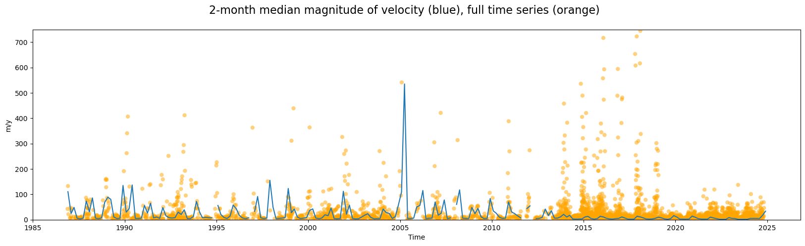
We can make a few observations:
Computing two-month median velocities makes it easier to see a somewhat periodic velocity signal
As expected, the median is highly sensitive to the density of observations; as such, it displays greater amplitude during periods with sparser observations. When the density of observations increases significantly in 2014, the amplitude of variability of the 2-month median curve decreases dramatically.
2) Grouped analysis by season#
Xarray’s groupby() functionality allows us to segment the dataset into different groups along given dimensions. Here, we use that to analyze seasonal velocity variability patterns:
seasons_gb = single_glacier_raster.groupby(single_glacier_raster.mid_date.dt.season).median()
#add attrs to gb object
seasons_gb.attrs = single_glacier_raster.attrs
#Reorder seasons
seasons_gb=seasons_gb.reindex({'season':['DJF','MAM','JJA','SON']})
seasons_gb
<xarray.Dataset> Size: 309kB
Dimensions: (x: 40, y: 37, season: 4)
Coordinates:
* x (x) float64 320B 7.843e+05 ... 7.889e+05
* y (y) float64 296B 3.316e+06 ... 3.311e+06
* season (season) <U3 48B 'DJF' 'MAM' 'JJA' 'SON'
mapping int64 8B 0
spatial_ref int64 8B 0
Data variables: (12/49)
M11 (season, y, x) float32 24kB nan nan ... nan nan
M11_dr_to_vr_factor (season) float32 16B nan nan nan nan
M12 (season, y, x) float32 24kB nan nan ... nan nan
M12_dr_to_vr_factor (season) float32 16B nan nan nan nan
chip_size_height (season, y, x) float32 24kB nan nan ... nan nan
chip_size_width (season, y, x) float32 24kB nan nan ... nan nan
... ...
vy_error_slow (season) float32 16B 8.2 4.8 4.2 9.1
vy_error_stationary (season) float32 16B 8.2 4.8 4.2 9.1
vy_stable_shift (season) float32 16B 0.1 0.0 0.0 0.5
vy_stable_shift_slow (season) float32 16B 0.1 0.0 0.0 0.5
vy_stable_shift_stationary (season) float32 16B 0.1 0.0 0.0 0.5
cov (season) float64 32B 0.0 0.0 0.0 0.0
Attributes: (12/19)
Conventions: CF-1.8
GDAL_AREA_OR_POINT: Area
author: ITS_LIVE, a NASA MEaSUREs project (its-live.j...
autoRIFT_parameter_file: http://its-live-data.s3.amazonaws.com/autorif...
datacube_software_version: 1.0
date_created: 25-Sep-2023 22:00:23
... ...
s3: s3://its-live-data/datacubes/v2/N30E090/ITS_L...
skipped_granules: s3://its-live-data/datacubes/v2/N30E090/ITS_L...
time_standard_img1: UTC
time_standard_img2: UTC
title: ITS_LIVE datacube of image pair velocities
url: https://its-live-data.s3.amazonaws.com/datacu...- x: 40
- y: 37
- season: 4
- x(x)float647.843e+05 7.844e+05 ... 7.889e+05
- axis :
- X
- description :
- x coordinate of projection
- long_name :
- x coordinate of projection
- standard_name :
- projection_x_coordinate
- units :
- metre
array([784252.5, 784372.5, 784492.5, 784612.5, 784732.5, 784852.5, 784972.5, 785092.5, 785212.5, 785332.5, 785452.5, 785572.5, 785692.5, 785812.5, 785932.5, 786052.5, 786172.5, 786292.5, 786412.5, 786532.5, 786652.5, 786772.5, 786892.5, 787012.5, 787132.5, 787252.5, 787372.5, 787492.5, 787612.5, 787732.5, 787852.5, 787972.5, 788092.5, 788212.5, 788332.5, 788452.5, 788572.5, 788692.5, 788812.5, 788932.5]) - y(y)float643.316e+06 3.316e+06 ... 3.311e+06
- axis :
- Y
- description :
- y coordinate of projection
- long_name :
- y coordinate of projection
- standard_name :
- projection_y_coordinate
- units :
- metre
array([3315787.5, 3315667.5, 3315547.5, 3315427.5, 3315307.5, 3315187.5, 3315067.5, 3314947.5, 3314827.5, 3314707.5, 3314587.5, 3314467.5, 3314347.5, 3314227.5, 3314107.5, 3313987.5, 3313867.5, 3313747.5, 3313627.5, 3313507.5, 3313387.5, 3313267.5, 3313147.5, 3313027.5, 3312907.5, 3312787.5, 3312667.5, 3312547.5, 3312427.5, 3312307.5, 3312187.5, 3312067.5, 3311947.5, 3311827.5, 3311707.5, 3311587.5, 3311467.5]) - season(season)<U3'DJF' 'MAM' 'JJA' 'SON'
- description :
- midpoint of image 1 and image 2 acquisition date and time with granule's centroid longitude and latitude as microseconds
- standard_name :
- image_pair_center_date_with_time_separation
array(['DJF', 'MAM', 'JJA', 'SON'], dtype='<U3')
- mapping()int640
- crs_wkt :
- PROJCS["WGS 84 / UTM zone 46N",GEOGCS["WGS 84",DATUM["WGS_1984",SPHEROID["WGS 84",6378137,298.257223563]],PRIMEM["Greenwich",0],UNIT["degree",0.0174532925199433,AUTHORITY["EPSG","9122"]],AUTHORITY["EPSG","4326"]],PROJECTION["Transverse_Mercator"],PARAMETER["latitude_of_origin",0],PARAMETER["central_meridian",93],PARAMETER["scale_factor",0.9996],PARAMETER["false_easting",500000],PARAMETER["false_northing",0],UNIT["metre",1],AXIS["Easting",EAST],AXIS["Northing",NORTH],AUTHORITY["EPSG","32646"]]
- semi_major_axis :
- 6378137.0
- semi_minor_axis :
- 6356752.314245179
- inverse_flattening :
- 298.257223563
- reference_ellipsoid_name :
- WGS 84
- longitude_of_prime_meridian :
- 0.0
- prime_meridian_name :
- Greenwich
- geographic_crs_name :
- WGS 84
- horizontal_datum_name :
- World Geodetic System 1984
- projected_crs_name :
- WGS 84 / UTM zone 46N
- grid_mapping_name :
- transverse_mercator
- latitude_of_projection_origin :
- 0.0
- longitude_of_central_meridian :
- 93.0
- false_easting :
- 500000.0
- false_northing :
- 0.0
- scale_factor_at_central_meridian :
- 0.9996
- spatial_ref :
- PROJCS["WGS 84 / UTM zone 46N",GEOGCS["WGS 84",DATUM["WGS_1984",SPHEROID["WGS 84",6378137,298.257223563]],PRIMEM["Greenwich",0],UNIT["degree",0.0174532925199433,AUTHORITY["EPSG","9122"]],AUTHORITY["EPSG","4326"]],PROJECTION["Transverse_Mercator"],PARAMETER["latitude_of_origin",0],PARAMETER["central_meridian",93],PARAMETER["scale_factor",0.9996],PARAMETER["false_easting",500000],PARAMETER["false_northing",0],UNIT["metre",1],AXIS["Easting",EAST],AXIS["Northing",NORTH],AUTHORITY["EPSG","32646"]]
array(0)
- spatial_ref()int640
- GeoTransform :
- 784192.5 120.0 0.0 3315847.5 0.0 -120.0
array(0)
- M11(season, y, x)float32nan nan nan nan ... nan nan nan nan
- description :
- conversion matrix element (1st row, 1st column) that can be multiplied with vx to give range pixel displacement dr (see Eq. A18 in https://www.mdpi.com/2072-4292/13/4/749)
- standard_name :
- conversion_matrix_element_11
- units :
- pixel/(meter/year)
array([[[nan, nan, nan, ..., 0., nan, nan], [nan, nan, nan, ..., 0., 0., nan], [nan, nan, nan, ..., 0., 0., nan], ..., [nan, nan, nan, ..., nan, nan, nan], [nan, nan, nan, ..., nan, nan, nan], [nan, nan, nan, ..., nan, nan, nan]], [[nan, nan, nan, ..., 0., nan, nan], [nan, nan, nan, ..., 0., 0., nan], [nan, nan, nan, ..., 0., 0., nan], ..., [nan, nan, nan, ..., nan, nan, nan], [nan, nan, nan, ..., nan, nan, nan], [nan, nan, nan, ..., nan, nan, nan]], [[nan, nan, nan, ..., 0., nan, nan], [nan, nan, nan, ..., 0., 0., nan], [nan, nan, nan, ..., 0., 0., nan], ..., [nan, nan, nan, ..., nan, nan, nan], [nan, nan, nan, ..., nan, nan, nan], [nan, nan, nan, ..., nan, nan, nan]], [[nan, nan, nan, ..., 0., nan, nan], [nan, nan, nan, ..., 0., 0., nan], [nan, nan, nan, ..., 0., 0., nan], ..., [nan, nan, nan, ..., nan, nan, nan], [nan, nan, nan, ..., nan, nan, nan], [nan, nan, nan, ..., nan, nan, nan]]], dtype=float32) - M11_dr_to_vr_factor(season)float32nan nan nan nan
- description :
- multiplicative factor that converts slant range pixel displacement dr to slant range velocity vr
- standard_name :
- M11_dr_to_vr_factor
- units :
- meter/(year*pixel)
array([nan, nan, nan, nan], dtype=float32)
- M12(season, y, x)float32nan nan nan nan ... nan nan nan nan
- description :
- conversion matrix element (1st row, 2nd column) that can be multiplied with vy to give range pixel displacement dr (see Eq. A18 in https://www.mdpi.com/2072-4292/13/4/749)
- standard_name :
- conversion_matrix_element_12
- units :
- pixel/(meter/year)
array([[[nan, nan, nan, ..., 0., nan, nan], [nan, nan, nan, ..., 0., 0., nan], [nan, nan, nan, ..., 0., 0., nan], ..., [nan, nan, nan, ..., nan, nan, nan], [nan, nan, nan, ..., nan, nan, nan], [nan, nan, nan, ..., nan, nan, nan]], [[nan, nan, nan, ..., 0., nan, nan], [nan, nan, nan, ..., 0., 0., nan], [nan, nan, nan, ..., 0., 0., nan], ..., [nan, nan, nan, ..., nan, nan, nan], [nan, nan, nan, ..., nan, nan, nan], [nan, nan, nan, ..., nan, nan, nan]], [[nan, nan, nan, ..., 0., nan, nan], [nan, nan, nan, ..., 0., 0., nan], [nan, nan, nan, ..., 0., 0., nan], ..., [nan, nan, nan, ..., nan, nan, nan], [nan, nan, nan, ..., nan, nan, nan], [nan, nan, nan, ..., nan, nan, nan]], [[nan, nan, nan, ..., 0., nan, nan], [nan, nan, nan, ..., 0., 0., nan], [nan, nan, nan, ..., 0., 0., nan], ..., [nan, nan, nan, ..., nan, nan, nan], [nan, nan, nan, ..., nan, nan, nan], [nan, nan, nan, ..., nan, nan, nan]]], dtype=float32) - M12_dr_to_vr_factor(season)float32nan nan nan nan
- description :
- multiplicative factor that converts slant range pixel displacement dr to slant range velocity vr
- standard_name :
- M12_dr_to_vr_factor
- units :
- meter/(year*pixel)
array([nan, nan, nan, nan], dtype=float32)
- chip_size_height(season, y, x)float32nan nan nan nan ... nan nan nan nan
- chip_size_coordinates :
- Optical data: chip_size_coordinates = 'image projection geometry: width = x, height = y'. Radar data: chip_size_coordinates = 'radar geometry: width = range, height = azimuth'
- description :
- height of search template (chip)
- standard_name :
- chip_size_height
- units :
- m
- y_pixel_size :
- 10.0
array([[[ nan, nan, nan, ..., 240., nan, nan], [ nan, nan, nan, ..., 240., 240., nan], [ nan, nan, nan, ..., 240., 240., nan], ..., [ nan, nan, nan, ..., nan, nan, nan], [ nan, nan, nan, ..., nan, nan, nan], [ nan, nan, nan, ..., nan, nan, nan]], [[ nan, nan, nan, ..., 240., nan, nan], [ nan, nan, nan, ..., 240., 240., nan], [ nan, nan, nan, ..., 480., 240., nan], ..., [ nan, nan, nan, ..., nan, nan, nan], [ nan, nan, nan, ..., nan, nan, nan], [ nan, nan, nan, ..., nan, nan, nan]], [[ nan, nan, nan, ..., 240., nan, nan], [ nan, nan, nan, ..., 240., 240., nan], [ nan, nan, nan, ..., 480., 240., nan], ..., [ nan, nan, nan, ..., nan, nan, nan], [ nan, nan, nan, ..., nan, nan, nan], [ nan, nan, nan, ..., nan, nan, nan]], [[ nan, nan, nan, ..., 240., nan, nan], [ nan, nan, nan, ..., 240., 240., nan], [ nan, nan, nan, ..., 480., 240., nan], ..., [ nan, nan, nan, ..., nan, nan, nan], [ nan, nan, nan, ..., nan, nan, nan], [ nan, nan, nan, ..., nan, nan, nan]]], dtype=float32) - chip_size_width(season, y, x)float32nan nan nan nan ... nan nan nan nan
- chip_size_coordinates :
- Optical data: chip_size_coordinates = 'image projection geometry: width = x, height = y'. Radar data: chip_size_coordinates = 'radar geometry: width = range, height = azimuth'
- description :
- width of search template (chip)
- standard_name :
- chip_size_width
- units :
- m
- x_pixel_size :
- 10.0
array([[[ nan, nan, nan, ..., 240., nan, nan], [ nan, nan, nan, ..., 240., 240., nan], [ nan, nan, nan, ..., 240., 240., nan], ..., [ nan, nan, nan, ..., nan, nan, nan], [ nan, nan, nan, ..., nan, nan, nan], [ nan, nan, nan, ..., nan, nan, nan]], [[ nan, nan, nan, ..., 240., nan, nan], [ nan, nan, nan, ..., 240., 240., nan], [ nan, nan, nan, ..., 480., 240., nan], ..., [ nan, nan, nan, ..., nan, nan, nan], [ nan, nan, nan, ..., nan, nan, nan], [ nan, nan, nan, ..., nan, nan, nan]], [[ nan, nan, nan, ..., 240., nan, nan], [ nan, nan, nan, ..., 240., 240., nan], [ nan, nan, nan, ..., 480., 240., nan], ..., [ nan, nan, nan, ..., nan, nan, nan], [ nan, nan, nan, ..., nan, nan, nan], [ nan, nan, nan, ..., nan, nan, nan]], [[ nan, nan, nan, ..., 240., nan, nan], [ nan, nan, nan, ..., 240., 240., nan], [ nan, nan, nan, ..., 480., 240., nan], ..., [ nan, nan, nan, ..., nan, nan, nan], [ nan, nan, nan, ..., nan, nan, nan], [ nan, nan, nan, ..., nan, nan, nan]]], dtype=float32) - date_dt(season)timedelta64[ns]164 days 23:54:22.500000 ... 215...
- description :
- time separation between acquisition of image 1 and image 2
- standard_name :
- image_pair_time_separation
array([14255662500000000, 26092618066406247, 27648121289062504, 18576217529296873], dtype='timedelta64[ns]') - floatingice(season, y, x)float32nan nan nan nan ... nan nan nan nan
- description :
- floating ice mask, 0 = non-floating-ice, 1 = floating-ice
- flag_meanings :
- non-ice ice
- flag_values :
- [0, 1]
- standard_name :
- floating ice mask
- url :
- https://its-live-data.s3.amazonaws.com/autorift_parameters/v001/N46_0120m_floatingice.tif
array([[[nan, nan, nan, ..., 0., nan, nan], [nan, nan, nan, ..., 0., 0., nan], [nan, nan, nan, ..., 0., 0., nan], ..., [nan, nan, nan, ..., nan, nan, nan], [nan, nan, nan, ..., nan, nan, nan], [nan, nan, nan, ..., nan, nan, nan]], [[nan, nan, nan, ..., 0., nan, nan], [nan, nan, nan, ..., 0., 0., nan], [nan, nan, nan, ..., 0., 0., nan], ..., [nan, nan, nan, ..., nan, nan, nan], [nan, nan, nan, ..., nan, nan, nan], [nan, nan, nan, ..., nan, nan, nan]], [[nan, nan, nan, ..., 0., nan, nan], [nan, nan, nan, ..., 0., 0., nan], [nan, nan, nan, ..., 0., 0., nan], ..., [nan, nan, nan, ..., nan, nan, nan], [nan, nan, nan, ..., nan, nan, nan], [nan, nan, nan, ..., nan, nan, nan]], [[nan, nan, nan, ..., 0., nan, nan], [nan, nan, nan, ..., 0., 0., nan], [nan, nan, nan, ..., 0., 0., nan], ..., [nan, nan, nan, ..., nan, nan, nan], [nan, nan, nan, ..., nan, nan, nan], [nan, nan, nan, ..., nan, nan, nan]]], dtype=float32) - interp_mask(season, y, x)float32nan nan nan nan ... nan nan nan nan
- description :
- light interpolation mask
- flag_meanings :
- measured interpolated
- flag_values :
- [0, 1]
- standard_name :
- interpolated_value_mask
array([[[nan, nan, nan, ..., 1., nan, nan], [nan, nan, nan, ..., 1., 1., nan], [nan, nan, nan, ..., 1., 1., nan], ..., [nan, nan, nan, ..., nan, nan, nan], [nan, nan, nan, ..., nan, nan, nan], [nan, nan, nan, ..., nan, nan, nan]], [[nan, nan, nan, ..., 1., nan, nan], [nan, nan, nan, ..., 1., 1., nan], [nan, nan, nan, ..., 1., 1., nan], ..., [nan, nan, nan, ..., nan, nan, nan], [nan, nan, nan, ..., nan, nan, nan], [nan, nan, nan, ..., nan, nan, nan]], [[nan, nan, nan, ..., 1., nan, nan], [nan, nan, nan, ..., 1., 1., nan], [nan, nan, nan, ..., 1., 1., nan], ..., [nan, nan, nan, ..., nan, nan, nan], [nan, nan, nan, ..., nan, nan, nan], [nan, nan, nan, ..., nan, nan, nan]], [[nan, nan, nan, ..., 1., nan, nan], [nan, nan, nan, ..., 1., 1., nan], [nan, nan, nan, ..., 1., 1., nan], ..., [nan, nan, nan, ..., nan, nan, nan], [nan, nan, nan, ..., nan, nan, nan], [nan, nan, nan, ..., nan, nan, nan]]], dtype=float32) - landice(season, y, x)float32nan nan nan nan ... nan nan nan nan
- description :
- land ice mask, 0 = non-land-ice, 1 = land-ice
- flag_meanings :
- non-ice ice
- flag_values :
- [0, 1]
- standard_name :
- land ice mask
- url :
- https://its-live-data.s3.amazonaws.com/autorift_parameters/v001/N46_0120m_landice.tif
array([[[nan, nan, nan, ..., 1., nan, nan], [nan, nan, nan, ..., 1., 1., nan], [nan, nan, nan, ..., 1., 1., nan], ..., [nan, nan, nan, ..., nan, nan, nan], [nan, nan, nan, ..., nan, nan, nan], [nan, nan, nan, ..., nan, nan, nan]], [[nan, nan, nan, ..., 1., nan, nan], [nan, nan, nan, ..., 1., 1., nan], [nan, nan, nan, ..., 1., 1., nan], ..., [nan, nan, nan, ..., nan, nan, nan], [nan, nan, nan, ..., nan, nan, nan], [nan, nan, nan, ..., nan, nan, nan]], [[nan, nan, nan, ..., 1., nan, nan], [nan, nan, nan, ..., 1., 1., nan], [nan, nan, nan, ..., 1., 1., nan], ..., [nan, nan, nan, ..., nan, nan, nan], [nan, nan, nan, ..., nan, nan, nan], [nan, nan, nan, ..., nan, nan, nan]], [[nan, nan, nan, ..., 1., nan, nan], [nan, nan, nan, ..., 1., 1., nan], [nan, nan, nan, ..., 1., 1., nan], ..., [nan, nan, nan, ..., nan, nan, nan], [nan, nan, nan, ..., nan, nan, nan], [nan, nan, nan, ..., nan, nan, nan]]], dtype=float32) - roi_valid_percentage(season)float3244.1 39.8 51.4 38.2
- description :
- percentage of pixels with a valid velocity estimate determined for the intersection of the full image pair footprint and the region of interest (roi) that defines where autoRIFT tried to estimate a velocity
- standard_name :
- region_of_interest_valid_pixel_percentage
array([44.1, 39.8, 51.4, 38.2], dtype=float32)
- stable_count_slow(season)float643.283e+04 3.262e+04 ... 3.227e+04
- description :
- number of valid pixels over slowest 25% of ice
- standard_name :
- stable_count_slow
- units :
- count
array([32830., 32625., 32189., 32272.])
- stable_count_stationary(season)float643.241e+04 3.256e+04 ... 3.227e+04
- description :
- number of valid pixels over stationary or slow-flowing surfaces
- standard_name :
- stable_count_stationary
- units :
- count
array([32408. , 32555.5, 32309. , 32274. ])
- stable_shift_flag(season)float641.0 1.0 1.0 1.0
- description :
- flag for applying velocity bias correction: 0 = no correction; 1 = correction from overlapping stable surface mask (stationary or slow-flowing surfaces with velocity < 15 m/yr)(top priority); 2 = correction from slowest 25% of overlapping velocities (second priority)
- standard_name :
- stable_shift_flag
array([1., 1., 1., 1.])
- v(season, y, x)float32nan nan nan nan ... nan nan nan nan
- description :
- velocity magnitude
- standard_name :
- land_ice_surface_velocity
- units :
- meter/year
array([[[nan, nan, nan, ..., 12., nan, nan], [nan, nan, nan, ..., 11., 12., nan], [nan, nan, nan, ..., 14., 14., nan], ..., [nan, nan, nan, ..., nan, nan, nan], [nan, nan, nan, ..., nan, nan, nan], [nan, nan, nan, ..., nan, nan, nan]], [[nan, nan, nan, ..., 6., nan, nan], [nan, nan, nan, ..., 6., 5., nan], [nan, nan, nan, ..., 6., 4., nan], ..., [nan, nan, nan, ..., nan, nan, nan], [nan, nan, nan, ..., nan, nan, nan], [nan, nan, nan, ..., nan, nan, nan]], [[nan, nan, nan, ..., 3., nan, nan], [nan, nan, nan, ..., 3., 3., nan], [nan, nan, nan, ..., 4., 3., nan], ..., [nan, nan, nan, ..., nan, nan, nan], [nan, nan, nan, ..., nan, nan, nan], [nan, nan, nan, ..., nan, nan, nan]], [[nan, nan, nan, ..., 10., nan, nan], [nan, nan, nan, ..., 11., 9., nan], [nan, nan, nan, ..., 12., 8., nan], ..., [nan, nan, nan, ..., nan, nan, nan], [nan, nan, nan, ..., nan, nan, nan], [nan, nan, nan, ..., nan, nan, nan]]], dtype=float32) - v_error(season, y, x)float32nan nan nan nan ... nan nan nan nan
- description :
- velocity magnitude error
- standard_name :
- velocity_error
- units :
- meter/year
array([[[nan, nan, nan, ..., 16., nan, nan], [nan, nan, nan, ..., 16., 16., nan], [nan, nan, nan, ..., 17., 16., nan], ..., [nan, nan, nan, ..., nan, nan, nan], [nan, nan, nan, ..., nan, nan, nan], [nan, nan, nan, ..., nan, nan, nan]], [[nan, nan, nan, ..., 6., nan, nan], [nan, nan, nan, ..., 5., 6., nan], [nan, nan, nan, ..., 7., 6., nan], ..., [nan, nan, nan, ..., nan, nan, nan], [nan, nan, nan, ..., nan, nan, nan], [nan, nan, nan, ..., nan, nan, nan]], [[nan, nan, nan, ..., 4., nan, nan], [nan, nan, nan, ..., 3., 3., nan], [nan, nan, nan, ..., 4., 3., nan], ..., [nan, nan, nan, ..., nan, nan, nan], [nan, nan, nan, ..., nan, nan, nan], [nan, nan, nan, ..., nan, nan, nan]], [[nan, nan, nan, ..., 12., nan, nan], [nan, nan, nan, ..., 12., 12., nan], [nan, nan, nan, ..., 13., 11., nan], ..., [nan, nan, nan, ..., nan, nan, nan], [nan, nan, nan, ..., nan, nan, nan], [nan, nan, nan, ..., nan, nan, nan]]], dtype=float32) - va(season, y, x)float32nan nan nan nan ... nan nan nan nan
- description :
- velocity in radar azimuth direction
array([[[ nan, nan, nan, ..., 0. , nan, nan], [ nan, nan, nan, ..., 9. , -7. , nan], [ nan, nan, nan, ..., -13. , 13. , nan], ..., [ nan, nan, nan, ..., nan, nan, nan], [ nan, nan, nan, ..., nan, nan, nan], [ nan, nan, nan, ..., nan, nan, nan]], [[ nan, nan, nan, ..., 1. , nan, nan], [ nan, nan, nan, ..., 33. , 26. , nan], [ nan, nan, nan, ..., 40. , 66. , nan], ..., [ nan, nan, nan, ..., nan, nan, nan], [ nan, nan, nan, ..., nan, nan, nan], [ nan, nan, nan, ..., nan, nan, nan]], [[ nan, nan, nan, ..., -13. , nan, nan], [ nan, nan, nan, ..., -11. , -21. , nan], [ nan, nan, nan, ..., 0. , 0. , nan], ..., [ nan, nan, nan, ..., nan, nan, nan], [ nan, nan, nan, ..., nan, nan, nan], [ nan, nan, nan, ..., nan, nan, nan]], [[ nan, nan, nan, ..., -2.5, nan, nan], [ nan, nan, nan, ..., -13. , -23.5, nan], [ nan, nan, nan, ..., -6.5, 6. , nan], ..., [ nan, nan, nan, ..., nan, nan, nan], [ nan, nan, nan, ..., nan, nan, nan], [ nan, nan, nan, ..., nan, nan, nan]]], dtype=float32) - va_error(season)float3260.25 72.75 50.05 59.35
- description :
- error for velocity in radar azimuth direction
- standard_name :
- va_error
- units :
- meter/year
array([60.25, 72.75, 50.05, 59.35], dtype=float32)
- va_error_modeled(season)float3264.4 64.4 64.4 64.4
- description :
- 1-sigma error calculated using a modeled error-dt relationship
- standard_name :
- va_error_modeled
- units :
- meter/year
array([64.4, 64.4, 64.4, 64.4], dtype=float32)
- va_error_slow(season)float3260.25 72.75 50.05 59.35
- description :
- RMSE over slowest 25% of retrieved velocities
- standard_name :
- va_error_slow
- units :
- meter/year
array([60.25, 72.75, 50.05, 59.35], dtype=float32)
- va_error_stationary(season)float3260.25 72.75 50.05 59.35
- description :
- RMSE over stable surfaces, stationary or slow-flowing surfaces with velocity < 15 m/yr identified from an external mask
- standard_name :
- va_error_stationary
- units :
- meter/year
array([60.25, 72.75, 50.05, 59.35], dtype=float32)
- va_stable_shift(season)float320.0 0.0 0.0 0.0
- description :
- applied va shift calibrated using pixels over stable or slow surfaces
- standard_name :
- va_stable_shift
- units :
- meter/year
array([0., 0., 0., 0.], dtype=float32)
- va_stable_shift_slow(season)float320.0 0.0 0.0 0.0
- description :
- va shift calibrated using valid pixels over slowest 25% of retrieved velocities
- standard_name :
- va_stable_shift_slow
- units :
- meter/year
array([0., 0., 0., 0.], dtype=float32)
- va_stable_shift_stationary(season)float320.0 0.0 0.0 0.0
- description :
- va shift calibrated using valid pixels over stable surfaces, stationary or slow-flowing surfaces with velocity < 15 m/yr identified from an external mask
- standard_name :
- va_stable_shift_stationary
- units :
- meter/year
array([0., 0., 0., 0.], dtype=float32)
- vr(season, y, x)float32nan nan nan nan ... nan nan nan nan
- description :
- velocity in radar range direction
array([[[ nan, nan, nan, ..., 6.5, nan, nan], [ nan, nan, nan, ..., 4. , 0. , nan], [ nan, nan, nan, ..., 2.5, 7. , nan], ..., [ nan, nan, nan, ..., nan, nan, nan], [ nan, nan, nan, ..., nan, nan, nan], [ nan, nan, nan, ..., nan, nan, nan]], [[ nan, nan, nan, ..., -9. , nan, nan], [ nan, nan, nan, ..., 0. , 0. , nan], [ nan, nan, nan, ..., 7. , 2. , nan], ..., [ nan, nan, nan, ..., nan, nan, nan], [ nan, nan, nan, ..., nan, nan, nan], [ nan, nan, nan, ..., nan, nan, nan]], [[ nan, nan, nan, ..., 6. , nan, nan], [ nan, nan, nan, ..., 7. , 3. , nan], [ nan, nan, nan, ..., 6. , 3. , nan], ..., [ nan, nan, nan, ..., nan, nan, nan], [ nan, nan, nan, ..., nan, nan, nan], [ nan, nan, nan, ..., nan, nan, nan]], [[ nan, nan, nan, ..., 0. , nan, nan], [ nan, nan, nan, ..., 4. , 1.5, nan], [ nan, nan, nan, ..., 0. , 4. , nan], ..., [ nan, nan, nan, ..., nan, nan, nan], [ nan, nan, nan, ..., nan, nan, nan], [ nan, nan, nan, ..., nan, nan, nan]]], dtype=float32) - vr_error(season)float3217.15 21.5 13.8 16.45
- description :
- error for velocity in radar range direction
- standard_name :
- vr_error
- units :
- meter/year
array([17.15, 21.5 , 13.8 , 16.45], dtype=float32)
- vr_error_modeled(season)float3219.8 19.8 19.8 19.8
- description :
- 1-sigma error calculated using a modeled error-dt relationship
- standard_name :
- vr_error_modeled
- units :
- meter/year
array([19.8, 19.8, 19.8, 19.8], dtype=float32)
- vr_error_slow(season)float3217.15 21.5 13.8 16.45
- description :
- RMSE over slowest 25% of retrieved velocities
- standard_name :
- vr_error_slow
- units :
- meter/year
array([17.15, 21.5 , 13.8 , 16.45], dtype=float32)
- vr_error_stationary(season)float3217.15 21.5 13.8 16.45
- description :
- RMSE over stable surfaces, stationary or slow-flowing surfaces with velocity < 15 m/yr identified from an external mask
- standard_name :
- vr_error_stationary
- units :
- meter/year
array([17.15, 21.5 , 13.8 , 16.45], dtype=float32)
- vr_stable_shift(season)float320.0 0.0 0.0 0.0
- description :
- applied vr shift calibrated using pixels over stable or slow surfaces
- standard_name :
- vr_stable_shift
- units :
- meter/year
array([0., 0., 0., 0.], dtype=float32)
- vr_stable_shift_slow(season)float320.0 0.0 0.0 0.0
- description :
- vr shift calibrated using valid pixels over slowest 25% of retrieved velocities
- standard_name :
- vr_stable_shift_slow
- units :
- meter/year
array([0., 0., 0., 0.], dtype=float32)
- vr_stable_shift_stationary(season)float320.0 0.0 0.0 0.0
- description :
- vr shift calibrated using valid pixels over stable surfaces, stationary or slow-flowing surfaces with velocity < 15 m/yr identified from an external mask
- standard_name :
- vr_stable_shift_stationary
- units :
- meter/year
array([0., 0., 0., 0.], dtype=float32)
- vx(season, y, x)float32nan nan nan nan ... nan nan nan nan
- description :
- velocity component in x direction
- standard_name :
- land_ice_surface_x_velocity
- units :
- meter/year
array([[[nan, nan, nan, ..., 1., nan, nan], [nan, nan, nan, ..., 0., 0., nan], [nan, nan, nan, ..., -1., -1., nan], ..., [nan, nan, nan, ..., nan, nan, nan], [nan, nan, nan, ..., nan, nan, nan], [nan, nan, nan, ..., nan, nan, nan]], [[nan, nan, nan, ..., 0., nan, nan], [nan, nan, nan, ..., 0., 0., nan], [nan, nan, nan, ..., 0., 0., nan], ..., [nan, nan, nan, ..., nan, nan, nan], [nan, nan, nan, ..., nan, nan, nan], [nan, nan, nan, ..., nan, nan, nan]], [[nan, nan, nan, ..., -1., nan, nan], [nan, nan, nan, ..., 0., 0., nan], [nan, nan, nan, ..., -1., 0., nan], ..., [nan, nan, nan, ..., nan, nan, nan], [nan, nan, nan, ..., nan, nan, nan], [nan, nan, nan, ..., nan, nan, nan]], [[nan, nan, nan, ..., -1., nan, nan], [nan, nan, nan, ..., 0., -1., nan], [nan, nan, nan, ..., -1., -2., nan], ..., [nan, nan, nan, ..., nan, nan, nan], [nan, nan, nan, ..., nan, nan, nan], [nan, nan, nan, ..., nan, nan, nan]]], dtype=float32) - vx_error(season)float325.4 3.4 3.3 6.0
- description :
- best estimate of x_velocity error: vx_error is populated according to the approach used for the velocity bias correction as indicated in "stable_shift_flag"
- standard_name :
- vx_error
- units :
- meter/year
array([5.4, 3.4, 3.3, 6. ], dtype=float32)
- vx_error_modeled(season)float3255.7 30.5 29.1 42.3
- description :
- 1-sigma error calculated using a modeled error-dt relationship
- standard_name :
- vx_error_modeled
- units :
- meter/year
array([55.7, 30.5, 29.1, 42.3], dtype=float32)
- vx_error_slow(season)float325.4 3.4 3.3 6.0
- description :
- RMSE over slowest 25% of retrieved velocities
- standard_name :
- vx_error_slow
- units :
- meter/year
array([5.4, 3.4, 3.3, 6. ], dtype=float32)
- vx_error_stationary(season)float325.4 3.4 3.3 6.0
- description :
- RMSE over stable surfaces, stationary or slow-flowing surfaces with velocity < 15 meter/year identified from an external mask
- standard_name :
- vx_error_stationary
- units :
- meter/year
array([5.4, 3.4, 3.3, 6. ], dtype=float32)
- vx_stable_shift(season)float320.0 0.0 0.0 -0.5
- description :
- applied vx shift calibrated using pixels over stable or slow surfaces
- standard_name :
- vx_stable_shift
- units :
- meter/year
array([ 0. , 0. , 0. , -0.5], dtype=float32)
- vx_stable_shift_slow(season)float320.0 0.0 0.0 -0.5
- description :
- vx shift calibrated using valid pixels over slowest 25% of retrieved velocities
- standard_name :
- vx_stable_shift_slow
- units :
- meter/year
array([ 0. , 0. , 0. , -0.5], dtype=float32)
- vx_stable_shift_stationary(season)float320.0 0.0 0.0 -0.5
- description :
- vx shift calibrated using valid pixels over stable surfaces, stationary or slow-flowing surfaces with velocity < 15 m/yr identified from an external mask
- standard_name :
- vx_stable_shift_stationary
- units :
- meter/year
array([ 0. , 0. , 0. , -0.5], dtype=float32)
- vy(season, y, x)float32nan nan nan nan ... nan nan nan nan
- description :
- velocity component in y direction
- standard_name :
- land_ice_surface_y_velocity
- units :
- meter/year
array([[[nan, nan, nan, ..., 3., nan, nan], [nan, nan, nan, ..., 3., 5., nan], [nan, nan, nan, ..., 1., 4., nan], ..., [nan, nan, nan, ..., nan, nan, nan], [nan, nan, nan, ..., nan, nan, nan], [nan, nan, nan, ..., nan, nan, nan]], [[nan, nan, nan, ..., 1., nan, nan], [nan, nan, nan, ..., 0., 0., nan], [nan, nan, nan, ..., 0., 0., nan], ..., [nan, nan, nan, ..., nan, nan, nan], [nan, nan, nan, ..., nan, nan, nan], [nan, nan, nan, ..., nan, nan, nan]], [[nan, nan, nan, ..., 0., nan, nan], [nan, nan, nan, ..., -1., 0., nan], [nan, nan, nan, ..., -1., 0., nan], ..., [nan, nan, nan, ..., nan, nan, nan], [nan, nan, nan, ..., nan, nan, nan], [nan, nan, nan, ..., nan, nan, nan]], [[nan, nan, nan, ..., -1., nan, nan], [nan, nan, nan, ..., -2., -1., nan], [nan, nan, nan, ..., -4., -1., nan], ..., [nan, nan, nan, ..., nan, nan, nan], [nan, nan, nan, ..., nan, nan, nan], [nan, nan, nan, ..., nan, nan, nan]]], dtype=float32) - vy_error(season)float328.2 4.8 4.2 9.1
- description :
- best estimate of y_velocity error: vy_error is populated according to the approach used for the velocity bias correction as indicated in "stable_shift_flag"
- standard_name :
- vy_error
- units :
- meter/year
array([8.2, 4.8, 4.2, 9.1], dtype=float32)
- vy_error_modeled(season)float3255.7 30.8 29.1 43.3
- description :
- 1-sigma error calculated using a modeled error-dt relationship
- standard_name :
- vy_error_modeled
- units :
- meter/year
array([55.7, 30.8, 29.1, 43.3], dtype=float32)
- vy_error_slow(season)float328.2 4.8 4.2 9.1
- description :
- RMSE over slowest 25% of retrieved velocities
- standard_name :
- vy_error_slow
- units :
- meter/year
array([8.2, 4.8, 4.2, 9.1], dtype=float32)
- vy_error_stationary(season)float328.2 4.8 4.2 9.1
- description :
- RMSE over stable surfaces, stationary or slow-flowing surfaces with velocity < 15 meter/year identified from an external mask
- standard_name :
- vy_error_stationary
- units :
- meter/year
array([8.2, 4.8, 4.2, 9.1], dtype=float32)
- vy_stable_shift(season)float320.1 0.0 0.0 0.5
- description :
- applied vy shift calibrated using pixels over stable or slow surfaces
- standard_name :
- vy_stable_shift
- units :
- meter/year
array([0.1, 0. , 0. , 0.5], dtype=float32)
- vy_stable_shift_slow(season)float320.1 0.0 0.0 0.5
- description :
- vy shift calibrated using valid pixels over slowest 25% of retrieved velocities
- standard_name :
- vy_stable_shift_slow
- units :
- meter/year
array([0.1, 0. , 0. , 0.5], dtype=float32)
- vy_stable_shift_stationary(season)float320.1 0.0 0.0 0.5
- description :
- vy shift calibrated using valid pixels over stable surfaces, stationary or slow-flowing surfaces with velocity < 15 m/yr identified from an external mask
- standard_name :
- vy_stable_shift_stationary
- units :
- meter/year
array([0.1, 0. , 0. , 0.5], dtype=float32)
- cov(season)float640.0 0.0 0.0 0.0
array([0., 0., 0., 0.])
- xPandasIndex
PandasIndex(Index([784252.5, 784372.5, 784492.5, 784612.5, 784732.5, 784852.5, 784972.5, 785092.5, 785212.5, 785332.5, 785452.5, 785572.5, 785692.5, 785812.5, 785932.5, 786052.5, 786172.5, 786292.5, 786412.5, 786532.5, 786652.5, 786772.5, 786892.5, 787012.5, 787132.5, 787252.5, 787372.5, 787492.5, 787612.5, 787732.5, 787852.5, 787972.5, 788092.5, 788212.5, 788332.5, 788452.5, 788572.5, 788692.5, 788812.5, 788932.5], dtype='float64', name='x')) - yPandasIndex
PandasIndex(Index([3315787.5, 3315667.5, 3315547.5, 3315427.5, 3315307.5, 3315187.5, 3315067.5, 3314947.5, 3314827.5, 3314707.5, 3314587.5, 3314467.5, 3314347.5, 3314227.5, 3314107.5, 3313987.5, 3313867.5, 3313747.5, 3313627.5, 3313507.5, 3313387.5, 3313267.5, 3313147.5, 3313027.5, 3312907.5, 3312787.5, 3312667.5, 3312547.5, 3312427.5, 3312307.5, 3312187.5, 3312067.5, 3311947.5, 3311827.5, 3311707.5, 3311587.5, 3311467.5], dtype='float64', name='y')) - seasonPandasIndex
PandasIndex(Index(['DJF', 'MAM', 'JJA', 'SON'], dtype='object', name='season'))
- Conventions :
- CF-1.8
- GDAL_AREA_OR_POINT :
- Area
- author :
- ITS_LIVE, a NASA MEaSUREs project (its-live.jpl.nasa.gov)
- autoRIFT_parameter_file :
- http://its-live-data.s3.amazonaws.com/autorift_parameters/v001/autorift_landice_0120m.shp
- datacube_software_version :
- 1.0
- date_created :
- 25-Sep-2023 22:00:23
- date_updated :
- 13-Nov-2024 00:08:07
- geo_polygon :
- [[95.06959008486952, 29.814255053135895], [95.32812062059084, 29.809951334550703], [95.58659184122865, 29.80514261876954], [95.84499718862224, 29.7998293459177], [96.10333011481168, 29.79401200205343], [96.11032804508507, 30.019297601073085], [96.11740568350054, 30.244573983323825], [96.12456379063154, 30.469841094022847], [96.1318031397002, 30.695098878594504], [95.87110827645229, 30.70112924501256], [95.61033817656023, 30.7066371044805], [95.34949964126946, 30.711621947056347], [95.08859948278467, 30.716083310981194], [95.08376623410525, 30.49063893600811], [95.07898726183609, 30.26518607254204], [95.0742620484426, 30.039724763743482], [95.06959008486952, 29.814255053135895]]
- institution :
- NASA Jet Propulsion Laboratory (JPL), California Institute of Technology
- latitude :
- 30.26
- longitude :
- 95.6
- proj_polygon :
- [[700000, 3300000], [725000.0, 3300000.0], [750000.0, 3300000.0], [775000.0, 3300000.0], [800000, 3300000], [800000.0, 3325000.0], [800000.0, 3350000.0], [800000.0, 3375000.0], [800000, 3400000], [775000.0, 3400000.0], [750000.0, 3400000.0], [725000.0, 3400000.0], [700000, 3400000], [700000.0, 3375000.0], [700000.0, 3350000.0], [700000.0, 3325000.0], [700000, 3300000]]
- projection :
- 32646
- s3 :
- s3://its-live-data/datacubes/v2/N30E090/ITS_LIVE_vel_EPSG32646_G0120_X750000_Y3350000.zarr
- skipped_granules :
- s3://its-live-data/datacubes/v2/N30E090/ITS_LIVE_vel_EPSG32646_G0120_X750000_Y3350000.json
- time_standard_img1 :
- UTC
- time_standard_img2 :
- UTC
- title :
- ITS_LIVE datacube of image pair velocities
- url :
- https://its-live-data.s3.amazonaws.com/datacubes/v2/N30E090/ITS_LIVE_vel_EPSG32646_G0120_X750000_Y3350000.zarr
This is cool; we’ve gone from our 3-d object with a very dense mid_date dimension to a 3-d object where the temporal aspect of the data is represented by 4 seasons.
In the above cell, we defined how we wanted to group our data (single_glacier_raster.mid_date.dt.season) and the reduction we wanted to apply to each group (median()). After the apply step, Xarray automatically combines the groups into a single object with a season dimension.
If you’d like to see another example of this with more detailed explanations, go here.
#Calculate magnitude on seasonal groupby object
seasons_vmag = calc_v_magnitude(seasons_gb)
Use another FacetGrid plot to visualize the seasons side-by-side:
fg = seasons_vmag.vmag.plot(
col='season',cbar_kwargs={'label':'Meters / year'}
)
fg.fig.suptitle('Seasonal median velocity magnitude', fontsize=16, y=1.05)
fg.fig.supxlabel('X-coordinate of projection (meters)', fontsize=12, y=-0.05)
fg.fig.supylabel('Y-coordinate of projection (meters)', fontsize=12, x=-0.02)
for i in range(len(fg.axs[0])):
fg.axs[0][i].set_ylabel(None)
fg.axs[0][i].set_xlabel(None)
fg.axs[0][i].tick_params(axis='x', labelrotation=45);
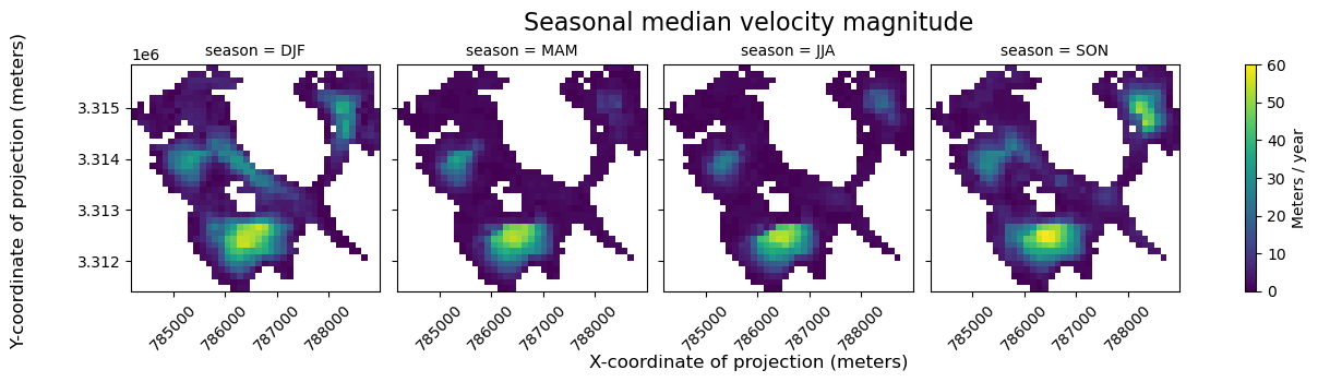
From the above FacetGrid plot, it appears that some regions of the glacier are very active (show high velocities) throughout the entire year. In other areas, it appears that glacier flow may be much more seasonal.
Conclusion
This was a deep dive in exploratory data analysis at the scale of an individual glacier. The last notebook in this chapter will demonstrate a regional-scale analysis.