Region-scale glacier analysis#
The previous notebook demonstrated using xarray to analyze surface velocity data for an individual glacier. This notebook will show how we can examine spatial variability in surface velocity within a group of glaciers. To do this we will use xarray as well as geopandas, geocube, and pandas. We will start by using .make_geocube() to rasterize a vector object in the shape of an ITS_LIVE velocity raster object. We will then use the rasterized vector to group the ITS_LIVE object by individual glaciers and then calculate summary statistics of surface velocity for each glacier. The goal in this work flow is to end up with a pandas dataframe where each row is an individual glacier and columns for various surface velocity summary statistics.
Learning goals#
Concepts#
Querying and accessing raster data from cloud object storage
Accessing and manipulating vector data
Handling coordinate reference information
Calculating and visualizing summary statistics
Techniques#
Other useful resources#
These are resources that contain additional examples and discussion of the content in this notebook and more.
How do I… this is very helpful!
Xarray High-level computational patterns discussion of concepts and associated code examples
Parallel computing with dask Xarray tutorial demonstrating wrapping of dask arrays
Software + Setup#
%xmode minimal
Exception reporting mode: Minimal
import os
import json
import urllib.request
import numpy as np
import xarray as xr
import rioxarray as rxr
import geopandas as gpd
import pandas as pd

import matplotlib.pyplot as plt

from shapely.geometry import Polygon
from shapely.geometry import Point
from geocube.api.core import make_geocube

%config InlineBackend.figure_format='retina'
import itslivetools
Accessing, reading raster data (ITS_LIVE velocity data)#
itslive_catalog = gpd.read_file('https://its-live-data.s3.amazonaws.com/datacubes/catalog_v02.json')
url = itslivetools.find_granule_by_point([95.180191, 30.645973])
url
'http://its-live-data.s3.amazonaws.com/datacubes/v2/N30E090/ITS_LIVE_vel_EPSG32646_G0120_X750000_Y3350000.zarr'
dc = itslivetools.read_in_s3(url)
dc
<xarray.Dataset>
Dimensions:                     (mid_date: 25243, y: 833, x: 833)
Coordinates:
  * mid_date                    (mid_date) datetime64[ns] 2022-06-07T04:21:44...
  * x                           (x) float64 7.001e+05 7.003e+05 ... 8e+05
  * y                           (y) float64 3.4e+06 3.4e+06 ... 3.3e+06 3.3e+06
Data variables: (12/60)
    M11                         (mid_date, y, x) float32 dask.array<chunksize=(25243, 30, 30), meta=np.ndarray>
    M11_dr_to_vr_factor         (mid_date) float32 dask.array<chunksize=(25243,), meta=np.ndarray>
    M12                         (mid_date, y, x) float32 dask.array<chunksize=(25243, 30, 30), meta=np.ndarray>
    M12_dr_to_vr_factor         (mid_date) float32 dask.array<chunksize=(25243,), meta=np.ndarray>
    acquisition_date_img1       (mid_date) datetime64[ns] dask.array<chunksize=(25243,), meta=np.ndarray>
    acquisition_date_img2       (mid_date) datetime64[ns] dask.array<chunksize=(25243,), meta=np.ndarray>
    ...                          ...
    vy_error_modeled            (mid_date) float32 dask.array<chunksize=(25243,), meta=np.ndarray>
    vy_error_slow               (mid_date) float32 dask.array<chunksize=(25243,), meta=np.ndarray>
    vy_error_stationary         (mid_date) float32 dask.array<chunksize=(25243,), meta=np.ndarray>
    vy_stable_shift             (mid_date) float32 dask.array<chunksize=(25243,), meta=np.ndarray>
    vy_stable_shift_slow        (mid_date) float32 dask.array<chunksize=(25243,), meta=np.ndarray>
    vy_stable_shift_stationary  (mid_date) float32 dask.array<chunksize=(25243,), meta=np.ndarray>
Attributes: (12/19)
    Conventions:                CF-1.8
    GDAL_AREA_OR_POINT:         Area
    author:                     ITS_LIVE, a NASA MEaSUREs project (its-live.j...
    autoRIFT_parameter_file:    http://its-live-data.s3.amazonaws.com/autorif...
    datacube_software_version:  1.0
    date_created:               25-Sep-2023 22:00:23
    ...                         ...
    s3:                         s3://its-live-data/datacubes/v2/N30E090/ITS_L...
    skipped_granules:           s3://its-live-data/datacubes/v2/N30E090/ITS_L...
    time_standard_img1:         UTC
    time_standard_img2:         UTC
    title:                      ITS_LIVE datacube of image pair velocities
url: https://its-live-data.s3.amazonaws.com/datacu...The mid_date dimension of the dc object isn’t in chronlogical order, so let’s sort by this dimension:
dc = dc.sortby('mid_date')
Create a crs object based on the projection data variable of the data cube (dc) object.
crs = f'EPSG:{dc.projection}'
crs
'EPSG:32646'
Reading vector data (glacier outlines)#
se_asia = gpd.read_parquet('rgi7_region15_south_asia_east.parquet')
se_asia.head(3)
| rgi_id | o1region | o2region | glims_id | anlys_id | subm_id | src_date | cenlon | cenlat | utm_zone | ... | zmin_m | zmax_m | zmed_m | zmean_m | slope_deg | aspect_deg | aspect_sec | dem_source | lmax_m | geometry | |
|---|---|---|---|---|---|---|---|---|---|---|---|---|---|---|---|---|---|---|---|---|---|
| 0 | RGI2000-v7.0-G-15-00001 | 15 | 15-01 | G078088E31398N | 866850 | 752 | 2002-07-10T00:00:00 | 78.087891 | 31.398046 | 44 | ... | 4662.2950 | 4699.2095 | 4669.4720 | 4671.4253 | 13.427070 | 122.267290 | 4 | COPDEM30 | 173 | POLYGON Z ((78.08905 31.39784 0.00000, 78.0889... |
| 1 | RGI2000-v7.0-G-15-00002 | 15 | 15-01 | G078125E31399N | 867227 | 752 | 2002-07-10T00:00:00 | 78.123699 | 31.397796 | 44 | ... | 4453.3584 | 4705.9920 | 4570.9473 | 4571.2770 | 22.822983 | 269.669144 | 7 | COPDEM30 | 1113 | POLYGON Z ((78.12556 31.40257 0.00000, 78.1255... |
| 2 | RGI2000-v7.0-G-15-00003 | 15 | 15-01 | G078128E31390N | 867273 | 752 | 2000-08-05T00:00:00 | 78.128510 | 31.390287 | 44 | ... | 4791.7593 | 4858.6807 | 4832.1836 | 4827.6700 | 15.626262 | 212.719681 | 6 | COPDEM30 | 327 | POLYGON Z ((78.12960 31.39093 0.00000, 78.1296... |
3 rows × 29 columns
How many glaciers are in this dataframe?
se_asia['rgi_id'].nunique()
18587
What coordinate reference system is this dataframe in?
se_asia.crs
<Geographic 2D CRS: EPSG:4326>
Name: WGS 84
Axis Info [ellipsoidal]:
- Lat[north]: Geodetic latitude (degree)
- Lon[east]: Geodetic longitude (degree)
Area of Use:
- name: World.
- bounds: (-180.0, -90.0, 180.0, 90.0)
Datum: World Geodetic System 1984 ensemble
- Ellipsoid: WGS 84
- Prime Meridian: Greenwich
The vector dataset is in WGS 84, meaning that its coordinates are in degrees latitude and longitude rather than meters N and E. We will project this dataset to match the projection of the raster dataset.
Handling projections#
Let’s project this dataframe to match the CRS of the itslive dataset
#project rgi data to match itslive
se_asia_prj = se_asia.to_crs(crs) #we know the epsg from the projection variable of the dc object
se_asia_prj.head(3)
| rgi_id | o1region | o2region | glims_id | anlys_id | subm_id | src_date | cenlon | cenlat | utm_zone | ... | zmin_m | zmax_m | zmed_m | zmean_m | slope_deg | aspect_deg | aspect_sec | dem_source | lmax_m | geometry | |
|---|---|---|---|---|---|---|---|---|---|---|---|---|---|---|---|---|---|---|---|---|---|
| 0 | RGI2000-v7.0-G-15-00001 | 15 | 15-01 | G078088E31398N | 866850 | 752 | 2002-07-10T00:00:00 | 78.087891 | 31.398046 | 44 | ... | 4662.2950 | 4699.2095 | 4669.4720 | 4671.4253 | 13.427070 | 122.267290 | 4 | COPDEM30 | 173 | POLYGON Z ((-924868.476 3571663.111 0.000, -92... |
| 1 | RGI2000-v7.0-G-15-00002 | 15 | 15-01 | G078125E31399N | 867227 | 752 | 2002-07-10T00:00:00 | 78.123699 | 31.397796 | 44 | ... | 4453.3584 | 4705.9920 | 4570.9473 | 4571.2770 | 22.822983 | 269.669144 | 7 | COPDEM30 | 1113 | POLYGON Z ((-921270.161 3571706.471 0.000, -92... |
| 2 | RGI2000-v7.0-G-15-00003 | 15 | 15-01 | G078128E31390N | 867273 | 752 | 2000-08-05T00:00:00 | 78.128510 | 31.390287 | 44 | ... | 4791.7593 | 4858.6807 | 4832.1836 | 4827.6700 | 15.626262 | 212.719681 | 6 | COPDEM30 | 327 | POLYGON Z ((-921061.745 3570342.665 0.000, -92... |
3 rows × 29 columns
se_asia_prj['rgi_id'].str.slice(18)
0        00001
1        00002
2        00003
3        00004
4        00005
         ...
18582    18583
18583    18584
18584    18585
18585    18586
18586    18587
Name: rgi_id, Length: 18587, dtype: object
Give each glacier (row) a unique integer key that is related to that glacier’s RGIId. We will use this later. Be careful that the RGI_int column is composed of integers not strings.
se_asia_prj['RGI_int'] = se_asia_prj['rgi_id'].str.slice(18,).astype(int)
se_asia_prj.RGI_int.dtype
dtype('int64')
To start with, we will look only at glaciers larger in area than 5km2. Subset the dataset to select for those glaciers
se_asia_prj = se_asia_prj.loc[se_asia_prj['area_km2'] > 5.]
se_asia_prj.head()
| rgi_id | o1region | o2region | glims_id | anlys_id | subm_id | src_date | cenlon | cenlat | utm_zone | ... | zmax_m | zmed_m | zmean_m | slope_deg | aspect_deg | aspect_sec | dem_source | lmax_m | geometry | RGI_int | |
|---|---|---|---|---|---|---|---|---|---|---|---|---|---|---|---|---|---|---|---|---|---|
| 59 | RGI2000-v7.0-G-15-00060 | 15 | 15-01 | G078577E31191N | 871719 | 752 | 2000-08-05T00:00:00 | 78.553292 | 31.174611 | 44 | ... | 6043.9136 | 5224.0610 | 5141.7990 | 17.677896 | 249.340500 | 7 | COPDEM90 | 13928 | POLYGON Z ((-880436.185 3544730.055 0.000, -88... | 60 |
| 66 | RGI2000-v7.0-G-15-00067 | 15 | 15-01 | G078523E31112N | 871438 | 752 | 2000-08-05T00:00:00 | 78.521258 | 31.116022 | 44 | ... | 5788.4610 | 4325.8790 | 4543.5195 | 18.882126 | 351.197868 | 1 | COPDEM30 | 7044 | POLYGON Z ((-888722.833 3534458.887 0.000, -88... | 67 |
| 157 | RGI2000-v7.0-G-15-00158 | 15 | 15-01 | G078843E31150N | 874200 | 752 | 2002-07-10T00:00:00 | 78.843177 | 31.150501 | 44 | ... | 5514.8880 | 5215.9690 | 5198.8105 | 12.894007 | 86.556990 | 3 | COPDEM30 | 4981 | POLYGON Z ((-856766.704 3533377.312 0.000, -85... | 158 |
| 209 | RGI2000-v7.0-G-15-00210 | 15 | 15-01 | G078779E31218N | 873926 | 752 | 2002-07-10T00:00:00 | 78.814979 | 31.218553 | 44 | ... | 6041.6123 | 5158.5570 | 5126.2070 | 12.179309 | 41.205524 | 2 | COPDEM90 | 18374 | POLYGON Z ((-869202.097 3540392.546 0.000, -86... | 210 |
| 229 | RGI2000-v7.0-G-15-00230 | 15 | 15-01 | G078544E31029N | 871696 | 752 | 2000-08-05T00:00:00 | 78.550250 | 31.038592 | 44 | ... | 6254.6704 | 5249.8203 | 5189.1060 | 20.423279 | 355.937175 | 1 | COPDEM90 | 10797 | POLYGON Z ((-884033.521 3525419.927 0.000, -88... | 230 |
5 rows × 30 columns
Next, want to subset the RGI dataset by the spatial extent of the ITS_LIVE data. First, get the bbox of the ITS_LIVE data as a vector
dc_bbox = itslivetools.get_bounds_polygon(dc)
dc_bbox.crs
<Projected CRS: EPSG:32646>
Name: WGS 84 / UTM zone 46N
Axis Info [cartesian]:
- E[east]: Easting (metre)
- N[north]: Northing (metre)
Area of Use:
- name: Between 90°E and 96°E, northern hemisphere between equator and 84°N, onshore and offshore. Bangladesh. Bhutan. China. Indonesia. Mongolia. Myanmar (Burma). Russian Federation.
- bounds: (90.0, 0.0, 96.0, 84.0)
Coordinate Operation:
- name: UTM zone 46N
- method: Transverse Mercator
Datum: World Geodetic System 1984 ensemble
- Ellipsoid: WGS 84
- Prime Meridian: Greenwich
Rasterize vector objects#
Subset RGI dataset:
To do this we will use a spatial join. Here we use an inner join but there are various methods to customize the spatial join operation. Find more info here.
rgi_sub = gpd.sjoin(se_asia_prj, dc_bbox, how='inner')
rgi_sub.head()
| rgi_id | o1region | o2region | glims_id | anlys_id | subm_id | src_date | cenlon | cenlat | utm_zone | ... | zmed_m | zmean_m | slope_deg | aspect_deg | aspect_sec | dem_source | lmax_m | geometry | RGI_int | index_right | |
|---|---|---|---|---|---|---|---|---|---|---|---|---|---|---|---|---|---|---|---|---|---|
| 11630 | RGI2000-v7.0-G-15-11631 | 15 | 15-03 | G095124E30309N | 927529 | 752 | 2003-07-24T00:00:00 | 95.106696 | 30.299816 | 46 | ... | 4881.6580 | 4866.093 | 21.731916 | 45.774250 | 2 | COPDEM90 | 19653 | POLYGON Z ((698995.535 3356459.046 0.000, 6990... | 11631 | 0 |
| 11631 | RGI2000-v7.0-G-15-11632 | 15 | 15-03 | G095138E30348N | 927618 | 752 | 2002-07-10T00:00:00 | 95.137897 | 30.347701 | 46 | ... | 5107.2480 | 5112.531 | 19.250132 | 212.500549 | 6 | COPDEM30 | 3968 | POLYGON Z ((705772.753 3360152.416 0.000, 7057... | 11632 | 0 |
| 11642 | RGI2000-v7.0-G-15-11643 | 15 | 15-03 | G095210E30329N | 927917 | 752 | 1997-08-24T00:00:00 | 95.209673 | 30.329234 | 46 | ... | 5023.0493 | 4969.326 | 23.261293 | 62.829437 | 2 | COPDEM30 | 5108 | POLYGON Z ((713890.435 3356601.497 0.000, 7138... | 11643 | 0 |
| 11672 | RGI2000-v7.0-G-15-11673 | 15 | 15-03 | G095324E30363N | 928296 | 752 | 2007-08-20T00:00:00 | 95.323927 | 30.363373 | 46 | ... | 5020.7920 | 5009.677 | 20.035536 | 43.020733 | 2 | COPDEM30 | 7190 | POLYGON Z ((720536.806 3361488.071 0.000, 7205... | 11673 | 0 |
| 11735 | RGI2000-v7.0-G-15-11736 | 15 | 15-03 | G095203E30636N | 927889 | 752 | 2002-07-10T00:00:00 | 95.203044 | 30.636060 | 46 | ... | 5383.6210 | 5355.023 | 14.739693 | 28.799190 | 2 | COPDEM30 | 4540 | POLYGON Z ((712706.746 3390103.661 0.000, 7126... | 11736 | 0 |
5 rows × 31 columns
Write crs of dc object. Event hough it is stored in the projection attribute, we want the projection to be stored as a rioxarray attribute so that it can be used in rioxarray methods.
dc = dc.rio.write_crs(crs)
rgi_sub = rgi_sub.drop('index_right', axis=1)
len(rgi_sub) # number of glaciers in the subset
28
Now, use the .make_geocube() function. This essentially takes a vector object (rgi_sub) and rasterizes it, returning an xarray object with the same structure as the object you provide for the like = argument (in our case that is dc). This example relies greatly on the zonal statistics example in the geocube documentation, which contains additional helpful details.
dc
<xarray.Dataset>
Dimensions:                     (mid_date: 25243, y: 833, x: 833)
Coordinates:
    mapping                     int64 0
  * mid_date                    (mid_date) datetime64[ns] 1986-09-11T03:31:15...
  * x                           (x) float64 7.001e+05 7.003e+05 ... 8e+05
  * y                           (y) float64 3.4e+06 3.4e+06 ... 3.3e+06 3.3e+06
Data variables: (12/59)
    M11                         (mid_date, y, x) float32 dask.array<chunksize=(25243, 30, 30), meta=np.ndarray>
    M11_dr_to_vr_factor         (mid_date) float32 dask.array<chunksize=(25243,), meta=np.ndarray>
    M12                         (mid_date, y, x) float32 dask.array<chunksize=(25243, 30, 30), meta=np.ndarray>
    M12_dr_to_vr_factor         (mid_date) float32 dask.array<chunksize=(25243,), meta=np.ndarray>
    acquisition_date_img1       (mid_date) datetime64[ns] dask.array<chunksize=(25243,), meta=np.ndarray>
    acquisition_date_img2       (mid_date) datetime64[ns] dask.array<chunksize=(25243,), meta=np.ndarray>
    ...                          ...
    vy_error_modeled            (mid_date) float32 dask.array<chunksize=(25243,), meta=np.ndarray>
    vy_error_slow               (mid_date) float32 dask.array<chunksize=(25243,), meta=np.ndarray>
    vy_error_stationary         (mid_date) float32 dask.array<chunksize=(25243,), meta=np.ndarray>
    vy_stable_shift             (mid_date) float32 dask.array<chunksize=(25243,), meta=np.ndarray>
    vy_stable_shift_slow        (mid_date) float32 dask.array<chunksize=(25243,), meta=np.ndarray>
    vy_stable_shift_stationary  (mid_date) float32 dask.array<chunksize=(25243,), meta=np.ndarray>
Attributes: (12/19)
    Conventions:                CF-1.8
    GDAL_AREA_OR_POINT:         Area
    author:                     ITS_LIVE, a NASA MEaSUREs project (its-live.j...
    autoRIFT_parameter_file:    http://its-live-data.s3.amazonaws.com/autorif...
    datacube_software_version:  1.0
    date_created:               25-Sep-2023 22:00:23
    ...                         ...
    s3:                         s3://its-live-data/datacubes/v2/N30E090/ITS_L...
    skipped_granules:           s3://its-live-data/datacubes/v2/N30E090/ITS_L...
    time_standard_img1:         UTC
    time_standard_img2:         UTC
    title:                      ITS_LIVE datacube of image pair velocities
url: https://its-live-data.s3.amazonaws.com/datacu...out_grid = make_geocube(
vector_data = rgi_sub,
measurements = ["RGI_int"],
like = dc
)
out_grid
<xarray.Dataset>
Dimensions:      (y: 833, x: 833)
Coordinates:
  * y            (y) float64 3.4e+06 3.4e+06 3.4e+06 ... 3.3e+06 3.3e+06 3.3e+06
  * x            (x) float64 7.001e+05 7.003e+05 7.004e+05 ... 7.999e+05 8e+05
    spatial_ref  int64 0
Data variables: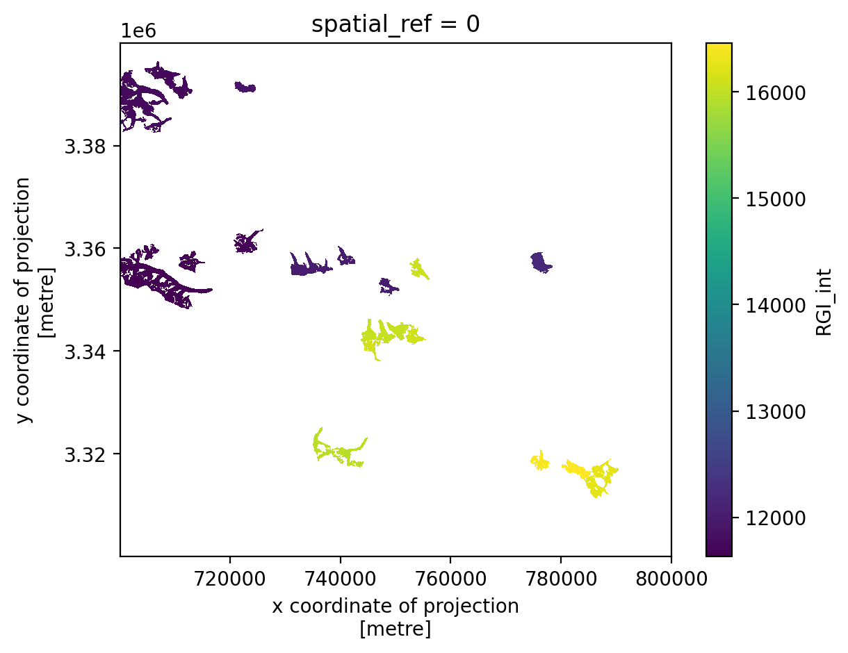
RGI_int (y, x) float64 nan nan nan nan nan nan ... nan nan nan nan nanNow each glacier in the geodataframe rgi_sub has been coded with a unique integer value that corresponds to that glacier’s Randolph Glacier Inventory ID.
out_grid.RGI_int.plot();
Before moving forward, we will take a temporal subset of the full dataset to make it a bit easier to work with. We will also compute the mean along the time dimension and calculate the magnitude of velocity using the velocity component variables.
Then, merge the rasterized vector and the dataset containing the velocity data into an xarray dataset:
dc_sub = dc.isel(mid_date=slice(400,500))
dc_sub_2d = dc_sub.mean(dim='mid_date')
dc_sub_2d['v_mag'] = np.sqrt(dc_sub_2d.vx**2+dc_sub_2d.vy**2)
Combining data#
Note
The following cell is very computationally intensive. It is executed here for the sake of demonstration but if you are running this code yourself be aware that it may not run/ may take a very long time to run. Consider taking a spatial subset of the dataset.
out_grid['v'] = (dc_sub_2d.v_mag.dims, dc_sub_2d.v_mag.values, dc_sub_2d.v_mag.attrs, dc_sub_2d.v_mag.encoding)
Assign the RGI_int object as a coordinate variable of the xarray.Dataset rather than a data_var.
out_grid = out_grid.assign_coords({'RGI_int':out_grid.RGI_int})
Grouping by RGI ID#
Now, we will use .groupby() to group the dataset by the RGI ID:
grouped_ID = out_grid.groupby('RGI_int')
<__array_function__ internals>:200: RuntimeWarning: invalid value encountered in cast
Calculating summary statistics#
Compute summary statistics for a single variable on the grouped object:
grid_mean_sp = grouped_ID.mean(dim=...).rename({'v': 'speed_mean'})
grid_median_sp = grouped_ID.median(dim=...).rename({'v': 'speed_median'})
grid_max_sp = grouped_ID.max(dim=...).rename({'v': 'speed_max'})
grid_min_sp = grouped_ID.min(dim=...).rename({'v': 'speed_min'})
Check if the data arrays (RGI_int) are equal, must be the case for xr.merge() in next step
print(grid_mean_sp.RGI_int.equals(grid_mean_sp.RGI_int))
print(grid_median_sp.RGI_int.equals(grid_median_sp.RGI_int))
print(grid_max_sp.RGI_int.equals(grid_max_sp.RGI_int))
print(grid_min_sp.RGI_int.equals(grid_min_sp.RGI_int))
True
True
True
True
Transitioning from ‘lazy’ operations to in-memory#
Merge and convert the lazy object to an in-memory equivalent using dask .compute(). Once it is in-memory, we can convert it to a pandas dataframe.
zonal_stats = xr.merge([grid_mean_sp, grid_median_sp, grid_max_sp, grid_min_sp]).compute()
zonal_stats_df = zonal_stats.to_dataframe()
zonal_stats_df = zonal_stats_df.reset_index()
zonal_stats_df = zonal_stats_df.drop(['spatial_ref'], axis=1)
zonal_stats_df
| RGI_int | speed_mean | speed_median | speed_max | speed_min | |
|---|---|---|---|---|---|
| 0 | 11631.0 | 43.229496 | 22.201803 | 357.174896 | 0.197642 |
| 1 | 11632.0 | 12.765533 | 11.598662 | 43.169296 | 0.258909 |
| 2 | 11643.0 | 18.185356 | 15.985531 | 87.176575 | 0.078567 |
| 3 | 11673.0 | 23.413357 | 17.378513 | 135.973846 | 0.225877 |
| 4 | 11736.0 | 18.280186 | 14.794738 | 117.458504 | 0.760345 |
| 5 | 11740.0 | 17.366793 | 15.020761 | 65.095032 | 1.400108 |
| 6 | 11746.0 | 17.681360 | 15.402331 | 65.298370 | 1.013794 |
| 7 | 11754.0 | 25.471052 | 19.809713 | 186.470001 | 0.552978 |
| 8 | 11759.0 | 19.896990 | 17.988567 | 91.692764 | 0.567878 |
| 9 | 11766.0 | 23.918291 | 20.536091 | 114.969078 | 1.363080 |
| 10 | 11895.0 | 12.812520 | 11.758823 | 53.096165 | 0.147059 |
| 11 | 11985.0 | 16.343838 | 14.805200 | 56.622963 | 0.124226 |
| 12 | 11994.0 | 22.481195 | 20.629883 | 61.390446 | 0.864832 |
| 13 | 11995.0 | 23.926825 | 17.536407 | 167.414978 | 0.400000 |
| 14 | 12015.0 | 18.282509 | 16.707451 | 66.150848 | 0.555556 |
| 15 | 12194.0 | 34.716423 | 27.442644 | 201.819031 | 0.903508 |
| 16 | 15962.0 | 27.554832 | 24.667400 | 163.135681 | 0.370370 |
| 17 | 15966.0 | 37.678925 | 23.696589 | 244.371765 | 0.581265 |
| 18 | 16033.0 | 24.644690 | 21.771954 | 94.401909 | 1.104536 |
| 19 | 16035.0 | 40.094566 | 31.823326 | 253.023712 | 1.788854 |
| 20 | 16036.0 | 32.543732 | 27.080856 | 122.827522 | 1.431782 |
| 21 | 16076.0 | 16.480865 | 14.312456 | 76.183197 | 0.859005 |
| 22 | 16108.0 | 21.932232 | 18.748005 | 95.795822 | 1.232693 |
| 23 | 16116.0 | 22.480335 | 18.999691 | 103.565865 | 0.500000 |
| 24 | 16255.0 | 27.704807 | 22.949593 | 110.771164 | 0.760559 |
| 25 | 16257.0 | 30.635042 | 24.937700 | 121.708672 | 0.840708 |
| 26 | 16408.0 | 29.208967 | 27.189728 | 85.190781 | 0.773067 |
| 27 | 16461.0 | 25.810692 | 24.004101 | 88.890732 | 1.607980 |
Now, make a new object (rgi_itslive) where you merge the zonal stats dataframe onto the GeoPandas.GeoDataframe object containing the RGI glacier outlines.
rgi_itslive = rgi_sub.loc[rgi_sub['area_km2'] > 5.]
rgi_itslive = pd.merge(rgi_sub, right = zonal_stats_df, how='inner', on='RGI_int')
rgi_itslive['rgi_id'].nunique()
28
Data visualization#
Now we can start to visualize the prepared dataset:
Pandas plotting#
fig, ax = plt.subplots()
sc = rgi_itslive.plot.scatter(x='speed_median',y = 'speed_mean', c = 'area_km2', ax=ax)
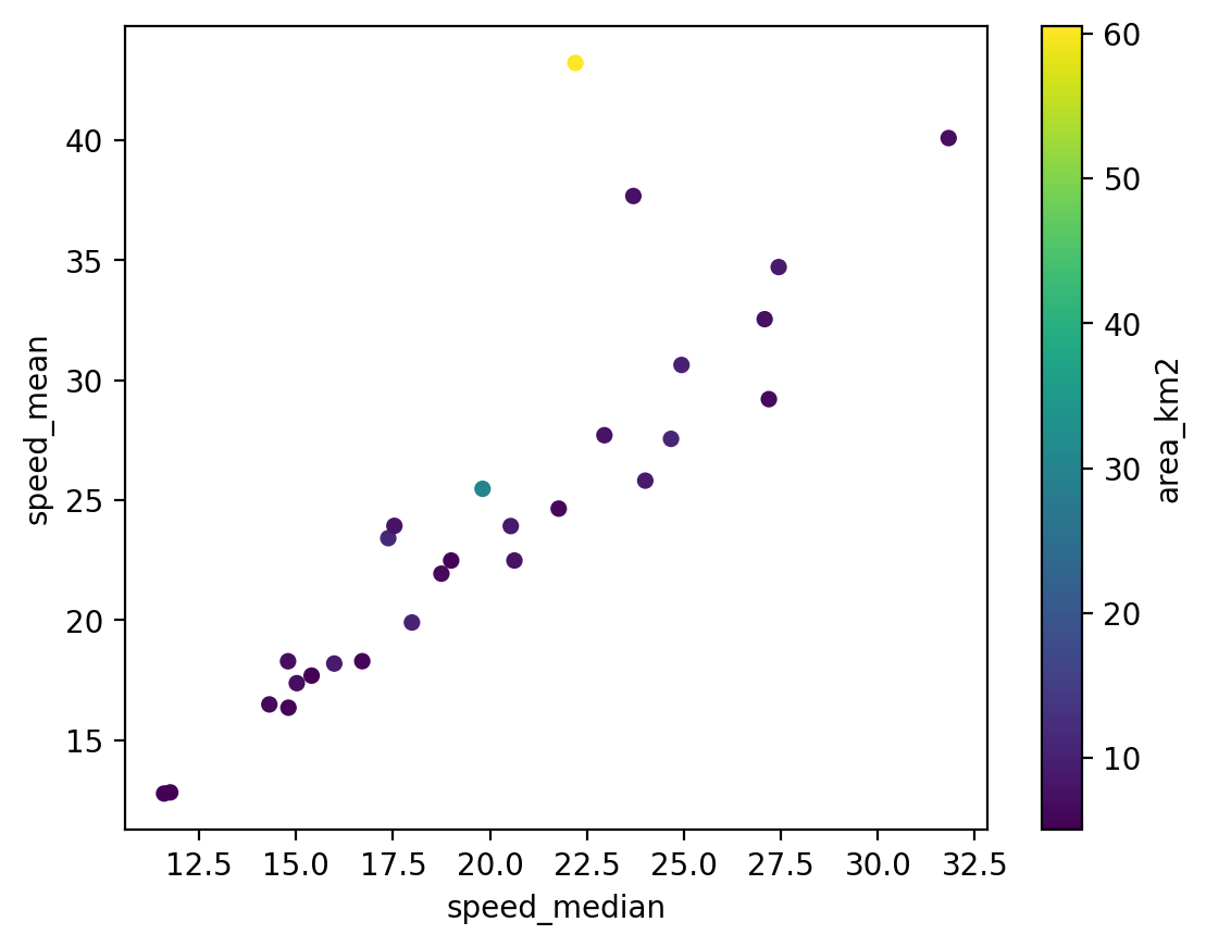
Now we have a plot but there is still more information we’d like to include. For example, the labelling could be improved to show units. Changing the x-axis and y-axis labels of the pandas dataframe plot is pretty simple:
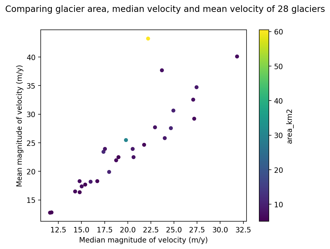
fig, ax = plt.subplots()
sc = rgi_itslive.plot.scatter(x='speed_median',y = 'speed_mean', c = 'area_km2', ax=ax)#.legend({'label':'test'})

fig.suptitle('Comparing glacier area, median velocity and mean velocity of 28 glaciers');
ax.set_ylabel('Mean magnitude of velocity (m/y)')
ax.set_xlabel('Median magnitude of velocity (m/y)');
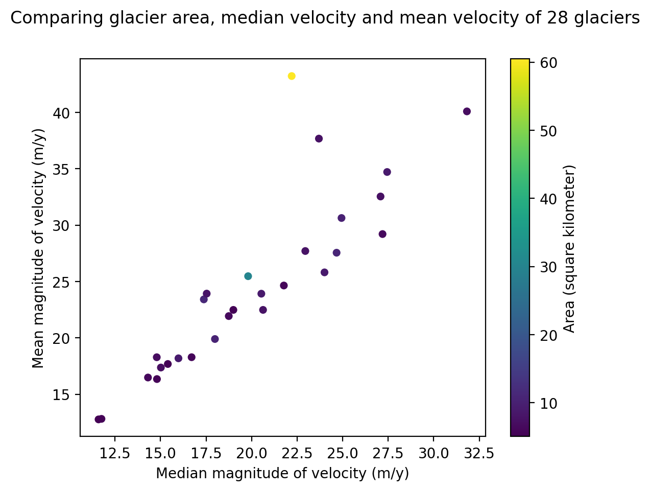
But this could still be improved. The Colormap that describes the area variable in this plot would be more descriptive if it included units. Here is one way of editing the Colormap label:
#see what axes are in your fig object
fig.get_axes()
[<Axes: xlabel='Median magnitude of velocity (m/y)', ylabel='Mean magnitude of velocity (m/y)'>,
 <Axes: label='<colorbar>', ylabel='area_km2'>]
#extract the one we are interested in (colorbar)
cax = fig.get_axes()[1]
cax
<Axes: label='<colorbar>', ylabel='area_km2'>
#modify colorbar label
cax.set_ylabel('Area (square kilometer)')
Text(1102.9030555555557, 0.5, 'Area (square kilometer)')
#all together
fig, ax = plt.subplots()
sc = rgi_itslive.plot.scatter(x='speed_median',y = 'speed_mean', c = 'area_km2', ax=ax)#.legend({'label':'test'})

fig.suptitle('Comparing glacier area, median velocity and mean velocity of 28 glaciers');
ax.set_ylabel('Mean magnitude of velocity (m/y)')
ax.set_xlabel('Median magnitude of velocity (m/y)');

cax = fig.get_axes()[1]
cax.set_ylabel('Area (square kilometer)');
Geopandas plotting#
In these plots, we are using the geometry information stored in the Geopandas.GeoDataFrame.
Static plots#
Specify the variable you’d like to observe in the plot. Set legend=True to add the colormap and pass legend_kwds as a dictionary to change the label and set other characteristics of the legend object.
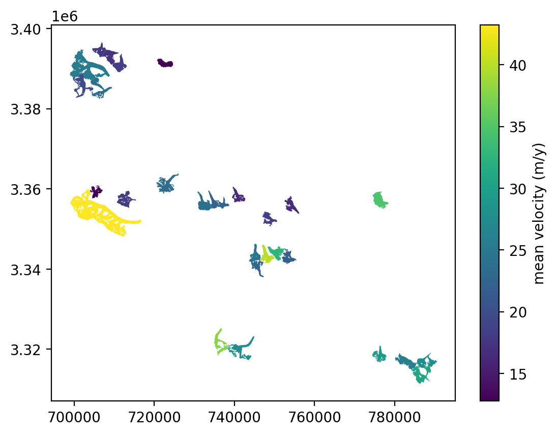
fig, ax = plt.subplots()
rgi_itslive.plot(ax=ax, column='speed_mean', legend=True,
                 legend_kwds={"label": "mean velocity (m/y)", "orientation": "vertical"},);
Interactive plots#
The geopandas.explore() method returns an interactive map of a Geopandas.GeoDataFrame - cool!
rgi_itslive.explore()
We can further customize the interactive plot:
rgi_itslive.explore('speed_median', cmap='inferno', style_kwds={'fillOpacity':0.7, 'stroke':False}, #stroke removes border around polygons, fillOpactiy sets opacity of polygons
                                                                                                   )
Awesome! We have encoded vector data onto a raster object that let’s us examine raster data for multiple spatial units simultaneously and explore a number of ways to visualize this data.