Accessing cloud-hosted ITS_LIVE data#
This notebook will demonstrate how to access cloud-hosted Inter-mission Time Series of Land Ice Velocity and Elevation (ITS_LIVE) data from AWS S3 buckets. Here, you will find examples of how to successfully access cloud-hosted data as well as some common errors and issues you may run into along the way, what they mean, and how to resolve them.
Learning goals#
Concepts#
Query and access cloud-optimized dataset from cloud object storage
Create a vector data object representing the footprint of a raster dataset
Preliminary visualization of data extent
Techniques#
Use Xarray to open Zarr datacube stored in AWS S3 bucket
Interactive data visualization with hvplot
Create Geopandas
geodataframefrom Xarrayxr.Datasetobject
Other useful resources#
These are resources that contain additional examples and discussion of the content in this notebook and more.
How do I… this is very helpful!
Xarray High-level computational patterns discussion of concepts and associated code examples
Parallel computing with dask Xarray tutorial demonstrating wrapping of dask arrays
Note
This tutorial was updated Fall 2023 to reflect changes to ITS_LIVE data urls and various software libraries
Software + Setup#
%load_ext watermark
%xmode minimal
Exception reporting mode: Minimal
import geopandas as gpd
import os
import numpy as np
import xarray as xr
import rioxarray as rxr

from shapely.geometry import Polygon
from shapely.geometry import Point
import hvplot.pandas
import hvplot.xarray

import json
import s3fs

%config InlineBackend.figure_format='retina'
%watermark
Last updated: 2024-02-20T22:53:17.102498-07:00

Python implementation: CPython
Python version       : 3.11.3
IPython version      : 8.13.2

Compiler    : GCC 11.3.0
OS          : Linux
Release     : 5.19.0-76051900-generic
Machine     : x86_64
Processor   : x86_64
CPU cores   : 16
Architecture: 64bit
%watermark --iversions
rioxarray: 0.14.1
geopandas: 0.13.0
xarray   : 2023.5.0
json     : 2.0.9
s3fs     : 2023.5.0
numpy    : 1.24.3
hvplot   : 0.8.4
ITS_LIVE data cube catalog#
The ITS_LIVE project details a number of data access options on their website. Here, we will be accessing ITS_LIVE data in the form of zarr data cubes that are stored in s3 buckets hosted by Amazon Web Services (AWS).
Let’s begin by looking at the GeoJSON data cubes catalog. Click this link to download the file. This catalog contains spatial information and properties of ITS_LIVE data cubes as well as the URL used to access each cube. Let’s take a look at the entry for a single data cube and the information that it contains:
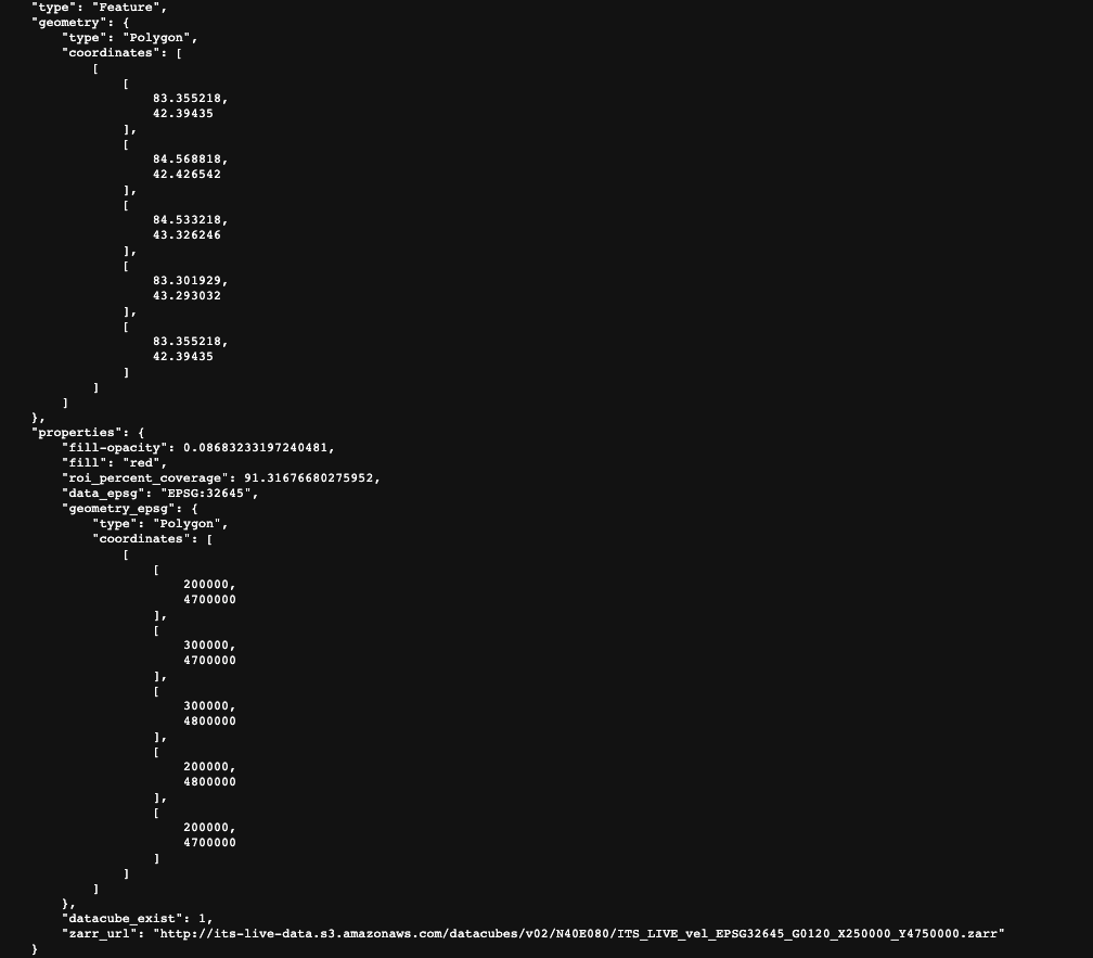
The top portion of the picture shows the spatial extent of the data cube in lat/lon units. Below that, we have properties such as the epsg code of the coordinate reference system, the spatial footprint in projected units and the url of the zarr object.
Let’s take a look at the url more in-depth:

From this link we can see that we are looking at its_live data located in an s3 bucket hosted by amazon AWS. We cans see that we’re looking in the data cube directory and what seems to be version 2. The next bit gives us information about the global location of the cube (N40E080). The actual file name ITS_LIVE_vel_EPSG32645_G0120_X250000_Y4750000.zarr tells us that we are looking at ice velocity data (its_live also has elevation data), in the CRS associated with EPSG 32645 (this code indicates UTM zone 45N). X250000_Y4750000 tells us more about the spatial footprint of the datacube within the UTM zone.
Accessing ITS_LIVE data from python#
We’ve found the url associated with the tile we want to access, let’s try to open the data cube using xarray:
url1 = 'http://its-live-data.s3.amazonaws.com/datacubes/v2/N30E090/ITS_LIVE_vel_EPSG32646_G0120_X750000_Y3350000.zarr'
dc1 = xr.open_dataset(url1)
syntax error, unexpected WORD_WORD, expecting SCAN_ATTR or SCAN_DATASET or SCAN_ERROR
context: <?xml^ version="1.0" encoding="UTF-8"?><Error><Code>PermanentRedirect</Code><Message>The bucket you are attempting to access must be addressed using the specified endpoint. Please send all future requests to this endpoint.</Message><Endpoint>its-live-data.s3-us-west-2.amazonaws.com</Endpoint><Bucket>its-live-data</Bucket><RequestId>3XZYGCPSMPFV5PCY</RequestId><HostId>jLB2uqxXYrbGGkN8zHbwzK50gl0sU9m2F/CX1pytA6nYqpxNQngEaLmXWdRr7ZKSbaWGyv+oJP8=</HostId></Error>
KeyError: [<class 'netCDF4._netCDF4.Dataset'>, ('http://its-live-data.s3.amazonaws.com/datacubes/v2/N30E090/ITS_LIVE_vel_EPSG32646_G0120_X750000_Y3350000.zarr',), 'r', (('clobber', True), ('diskless', False), ('format', 'NETCDF4'), ('persist', False)), '682a26e7-d3ba-4824-a515-2b19e004e1a1']


During handling of the above exception, another exception occurred:

OSError: [Errno -72] NetCDF: Malformed or inaccessible DAP2 DDS or DAP4 DMR response: 'http://its-live-data.s3.amazonaws.com/datacubes/v2/N30E090/ITS_LIVE_vel_EPSG32646_G0120_X750000_Y3350000.zarr'
As you can see, this doesn’t quite work. Passing the url to xr.open_dataset() without specifying a backend, xarray will expect a netcdf file. Because we’re trying to open a zarr file we need to add an additional argument to xr.open_dataset(), shown in the next code cell. You can find more information here. In the following cell, the argument chunks="auto" is passed, which introduces dask into our workflow.
dc1 = xr.open_dataset(url1, engine= 'zarr', chunks="auto")
                                   # storage_options = {'anon':True}) <-- as of Fall 2023 this no longer needed
dc1
<xarray.Dataset>
Dimensions:                     (mid_date: 25243, y: 833, x: 833)
Coordinates:
  * mid_date                    (mid_date) datetime64[ns] 2022-06-07T04:21:44...
  * x                           (x) float64 7.001e+05 7.003e+05 ... 8e+05
  * y                           (y) float64 3.4e+06 3.4e+06 ... 3.3e+06 3.3e+06
Data variables: (12/60)
    M11                         (mid_date, y, x) float32 dask.array<chunksize=(25243, 30, 30), meta=np.ndarray>
    M11_dr_to_vr_factor         (mid_date) float32 dask.array<chunksize=(25243,), meta=np.ndarray>
    M12                         (mid_date, y, x) float32 dask.array<chunksize=(25243, 30, 30), meta=np.ndarray>
    M12_dr_to_vr_factor         (mid_date) float32 dask.array<chunksize=(25243,), meta=np.ndarray>
    acquisition_date_img1       (mid_date) datetime64[ns] dask.array<chunksize=(25243,), meta=np.ndarray>
    acquisition_date_img2       (mid_date) datetime64[ns] dask.array<chunksize=(25243,), meta=np.ndarray>
    ...                          ...
    vy_error_modeled            (mid_date) float32 dask.array<chunksize=(25243,), meta=np.ndarray>
    vy_error_slow               (mid_date) float32 dask.array<chunksize=(25243,), meta=np.ndarray>
    vy_error_stationary         (mid_date) float32 dask.array<chunksize=(25243,), meta=np.ndarray>
    vy_stable_shift             (mid_date) float32 dask.array<chunksize=(25243,), meta=np.ndarray>
    vy_stable_shift_slow        (mid_date) float32 dask.array<chunksize=(25243,), meta=np.ndarray>
    vy_stable_shift_stationary  (mid_date) float32 dask.array<chunksize=(25243,), meta=np.ndarray>
Attributes: (12/19)
    Conventions:                CF-1.8
    GDAL_AREA_OR_POINT:         Area
    author:                     ITS_LIVE, a NASA MEaSUREs project (its-live.j...
    autoRIFT_parameter_file:    http://its-live-data.s3.amazonaws.com/autorif...
    datacube_software_version:  1.0
    date_created:               25-Sep-2023 22:00:23
    ...                         ...
    s3:                         s3://its-live-data/datacubes/v2/N30E090/ITS_L...
    skipped_granules:           s3://its-live-data/datacubes/v2/N30E090/ITS_L...
    time_standard_img1:         UTC
    time_standard_img2:         UTC
    title:                      ITS_LIVE datacube of image pair velocities
url: https://its-live-data.s3.amazonaws.com/datacu...- mid_date: 25243
- y: 833
- x: 833
- mid_date(mid_date)datetime64[ns]2022-06-07T04:21:44.211208960 .....
- description :
- midpoint of image 1 and image 2 acquisition date and time with granule's centroid longitude and latitude as microseconds
- standard_name :
- image_pair_center_date_with_time_separation
array(['2022-06-07T04:21:44.211208960', '2018-04-14T04:18:49.171219968', '2017-02-10T16:15:50.660901120', ..., '2013-05-20T04:08:31.155972096', '2015-10-17T04:11:05.527512064', '2015-11-10T04:11:15.457366016'], dtype='datetime64[ns]') - x(x)float647.001e+05 7.003e+05 ... 8e+05
- description :
- x coordinate of projection
- standard_name :
- projection_x_coordinate
array([700132.5, 700252.5, 700372.5, ..., 799732.5, 799852.5, 799972.5])
- y(y)float643.4e+06 3.4e+06 ... 3.3e+06 3.3e+06
- description :
- y coordinate of projection
- standard_name :
- projection_y_coordinate
array([3399907.5, 3399787.5, 3399667.5, ..., 3300307.5, 3300187.5, 3300067.5])
- M11(mid_date, y, x)float32dask.array<chunksize=(25243, 30, 30), meta=np.ndarray>
- description :
- conversion matrix element (1st row, 1st column) that can be multiplied with vx to give range pixel displacement dr (see Eq. A18 in https://www.mdpi.com/2072-4292/13/4/749)
- grid_mapping :
- mapping
- standard_name :
- conversion_matrix_element_11
- units :
- pixel/(meter/year)
Array Chunk Bytes 65.25 GiB 86.66 MiB Shape (25243, 833, 833) (25243, 30, 30) Dask graph 784 chunks in 2 graph layers Data type float32 numpy.ndarray - M11_dr_to_vr_factor(mid_date)float32dask.array<chunksize=(25243,), meta=np.ndarray>
- description :
- multiplicative factor that converts slant range pixel displacement dr to slant range velocity vr
- standard_name :
- M11_dr_to_vr_factor
- units :
- meter/(year*pixel)
Array Chunk Bytes 98.61 kiB 98.61 kiB Shape (25243,) (25243,) Dask graph 1 chunks in 2 graph layers Data type float32 numpy.ndarray - M12(mid_date, y, x)float32dask.array<chunksize=(25243, 30, 30), meta=np.ndarray>
- description :
- conversion matrix element (1st row, 2nd column) that can be multiplied with vy to give range pixel displacement dr (see Eq. A18 in https://www.mdpi.com/2072-4292/13/4/749)
- grid_mapping :
- mapping
- standard_name :
- conversion_matrix_element_12
- units :
- pixel/(meter/year)
Array Chunk Bytes 65.25 GiB 86.66 MiB Shape (25243, 833, 833) (25243, 30, 30) Dask graph 784 chunks in 2 graph layers Data type float32 numpy.ndarray - M12_dr_to_vr_factor(mid_date)float32dask.array<chunksize=(25243,), meta=np.ndarray>
- description :
- multiplicative factor that converts slant range pixel displacement dr to slant range velocity vr
- standard_name :
- M12_dr_to_vr_factor
- units :
- meter/(year*pixel)
Array Chunk Bytes 98.61 kiB 98.61 kiB Shape (25243,) (25243,) Dask graph 1 chunks in 2 graph layers Data type float32 numpy.ndarray - acquisition_date_img1(mid_date)datetime64[ns]dask.array<chunksize=(25243,), meta=np.ndarray>
- description :
- acquisition date and time of image 1
- standard_name :
- image1_acquition_date
Array Chunk Bytes 197.21 kiB 197.21 kiB Shape (25243,) (25243,) Dask graph 1 chunks in 2 graph layers Data type datetime64[ns] numpy.ndarray - acquisition_date_img2(mid_date)datetime64[ns]dask.array<chunksize=(25243,), meta=np.ndarray>
- description :
- acquisition date and time of image 2
- standard_name :
- image2_acquition_date
Array Chunk Bytes 197.21 kiB 197.21 kiB Shape (25243,) (25243,) Dask graph 1 chunks in 2 graph layers Data type datetime64[ns] numpy.ndarray - autoRIFT_software_version(mid_date)<U5dask.array<chunksize=(25243,), meta=np.ndarray>
- description :
- version of autoRIFT software
- standard_name :
- autoRIFT_software_version
Array Chunk Bytes 493.03 kiB 493.03 kiB Shape (25243,) (25243,) Dask graph 1 chunks in 2 graph layers Data type - chip_size_height(mid_date, y, x)float32dask.array<chunksize=(25243, 30, 30), meta=np.ndarray>
- chip_size_coordinates :
- Optical data: chip_size_coordinates = 'image projection geometry: width = x, height = y'. Radar data: chip_size_coordinates = 'radar geometry: width = range, height = azimuth'
- description :
- height of search template (chip)
- grid_mapping :
- mapping
- standard_name :
- chip_size_height
- units :
- m
- y_pixel_size :
- 10.0
Array Chunk Bytes 65.25 GiB 86.66 MiB Shape (25243, 833, 833) (25243, 30, 30) Dask graph 784 chunks in 2 graph layers Data type float32 numpy.ndarray - chip_size_width(mid_date, y, x)float32dask.array<chunksize=(25243, 30, 30), meta=np.ndarray>
- chip_size_coordinates :
- Optical data: chip_size_coordinates = 'image projection geometry: width = x, height = y'. Radar data: chip_size_coordinates = 'radar geometry: width = range, height = azimuth'
- description :
- width of search template (chip)
- grid_mapping :
- mapping
- standard_name :
- chip_size_width
- units :
- m
- x_pixel_size :
- 10.0
Array Chunk Bytes 65.25 GiB 86.66 MiB Shape (25243, 833, 833) (25243, 30, 30) Dask graph 784 chunks in 2 graph layers Data type float32 numpy.ndarray - date_center(mid_date)datetime64[ns]dask.array<chunksize=(25243,), meta=np.ndarray>
- description :
- midpoint of image 1 and image 2 acquisition date
- standard_name :
- image_pair_center_date
Array Chunk Bytes 197.21 kiB 197.21 kiB Shape (25243,) (25243,) Dask graph 1 chunks in 2 graph layers Data type datetime64[ns] numpy.ndarray - date_dt(mid_date)timedelta64[ns]dask.array<chunksize=(25243,), meta=np.ndarray>
- description :
- time separation between acquisition of image 1 and image 2
- standard_name :
- image_pair_time_separation
Array Chunk Bytes 197.21 kiB 197.21 kiB Shape (25243,) (25243,) Dask graph 1 chunks in 2 graph layers Data type timedelta64[ns] numpy.ndarray - floatingice(y, x)float32dask.array<chunksize=(833, 833), meta=np.ndarray>
- description :
- floating ice mask, 0 = non-floating-ice, 1 = floating-ice
- flag_meanings :
- non-ice ice
- flag_values :
- [0, 1]
- grid_mapping :
- mapping
- standard_name :
- floating ice mask
- url :
- https://its-live-data.s3.amazonaws.com/autorift_parameters/v001/N46_0120m_floatingice.tif
Array Chunk Bytes 2.65 MiB 2.65 MiB Shape (833, 833) (833, 833) Dask graph 1 chunks in 2 graph layers Data type float32 numpy.ndarray - granule_url(mid_date)<U1024dask.array<chunksize=(25243,), meta=np.ndarray>
- description :
- original granule URL
- standard_name :
- granule_url
Array Chunk Bytes 98.61 MiB 98.61 MiB Shape (25243,) (25243,) Dask graph 1 chunks in 2 graph layers Data type - interp_mask(mid_date, y, x)float32dask.array<chunksize=(25243, 30, 30), meta=np.ndarray>
- description :
- light interpolation mask
- flag_meanings :
- measured interpolated
- flag_values :
- [0, 1]
- grid_mapping :
- mapping
- standard_name :
- interpolated_value_mask
Array Chunk Bytes 65.25 GiB 86.66 MiB Shape (25243, 833, 833) (25243, 30, 30) Dask graph 784 chunks in 2 graph layers Data type float32 numpy.ndarray - landice(y, x)float32dask.array<chunksize=(833, 833), meta=np.ndarray>
- description :
- land ice mask, 0 = non-land-ice, 1 = land-ice
- flag_meanings :
- non-ice ice
- flag_values :
- [0, 1]
- grid_mapping :
- mapping
- standard_name :
- land ice mask
- url :
- https://its-live-data.s3.amazonaws.com/autorift_parameters/v001/N46_0120m_landice.tif
Array Chunk Bytes 2.65 MiB 2.65 MiB Shape (833, 833) (833, 833) Dask graph 1 chunks in 2 graph layers Data type float32 numpy.ndarray - mapping()<U1...
- GeoTransform :
- 700072.5 120.0 0 3399967.5 0 -120.0
- crs_wkt :
- PROJCS["WGS 84 / UTM zone 46N",GEOGCS["WGS 84",DATUM["WGS_1984",SPHEROID["WGS 84",6378137,298.257223563,AUTHORITY["EPSG","7030"]],AUTHORITY["EPSG","6326"]],PRIMEM["Greenwich",0,AUTHORITY["EPSG","8901"]],UNIT["degree",0.0174532925199433,AUTHORITY["EPSG","9122"]],AUTHORITY["EPSG","4326"]],PROJECTION["Transverse_Mercator"],PARAMETER["latitude_of_origin",0],PARAMETER["central_meridian",93],PARAMETER["scale_factor",0.9996],PARAMETER["false_easting",500000],PARAMETER["false_northing",0],UNIT["metre",1,AUTHORITY["EPSG","9001"]],AXIS["Easting",EAST],AXIS["Northing",NORTH],AUTHORITY["EPSG","32646"]]
- false_easting :
- 500000.0
- false_northing :
- 0.0
- grid_mapping_name :
- universal_transverse_mercator
- inverse_flattening :
- 298.257223563
- latitude_of_projection_origin :
- 0.0
- longitude_of_central_meridian :
- 93.0
- proj4text :
- +proj=utm +zone=46 +datum=WGS84 +units=m +no_defs
- scale_factor_at_central_meridian :
- 0.9996
- semi_major_axis :
- 6378137.0
- spatial_epsg :
- 32646
- spatial_ref :
- PROJCS["WGS 84 / UTM zone 46N",GEOGCS["WGS 84",DATUM["WGS_1984",SPHEROID["WGS 84",6378137,298.257223563,AUTHORITY["EPSG","7030"]],AUTHORITY["EPSG","6326"]],PRIMEM["Greenwich",0,AUTHORITY["EPSG","8901"]],UNIT["degree",0.0174532925199433,AUTHORITY["EPSG","9122"]],AUTHORITY["EPSG","4326"]],PROJECTION["Transverse_Mercator"],PARAMETER["latitude_of_origin",0],PARAMETER["central_meridian",93],PARAMETER["scale_factor",0.9996],PARAMETER["false_easting",500000],PARAMETER["false_northing",0],UNIT["metre",1,AUTHORITY["EPSG","9001"]],AXIS["Easting",EAST],AXIS["Northing",NORTH],AUTHORITY["EPSG","32646"]]
- utm_zone_number :
- 46.0
[1 values with dtype=<U1]
- mission_img1(mid_date)<U1dask.array<chunksize=(25243,), meta=np.ndarray>
- description :
- id of the mission that acquired image 1
- standard_name :
- image1_mission
Array Chunk Bytes 98.61 kiB 98.61 kiB Shape (25243,) (25243,) Dask graph 1 chunks in 2 graph layers Data type - mission_img2(mid_date)<U1dask.array<chunksize=(25243,), meta=np.ndarray>
- description :
- id of the mission that acquired image 2
- standard_name :
- image2_mission
Array Chunk Bytes 98.61 kiB 98.61 kiB Shape (25243,) (25243,) Dask graph 1 chunks in 2 graph layers Data type - roi_valid_percentage(mid_date)float32dask.array<chunksize=(25243,), meta=np.ndarray>
- description :
- percentage of pixels with a valid velocity estimate determined for the intersection of the full image pair footprint and the region of interest (roi) that defines where autoRIFT tried to estimate a velocity
- standard_name :
- region_of_interest_valid_pixel_percentage
Array Chunk Bytes 98.61 kiB 98.61 kiB Shape (25243,) (25243,) Dask graph 1 chunks in 2 graph layers Data type float32 numpy.ndarray - satellite_img1(mid_date)<U2dask.array<chunksize=(25243,), meta=np.ndarray>
- description :
- id of the satellite that acquired image 1
- standard_name :
- image1_satellite
Array Chunk Bytes 197.21 kiB 197.21 kiB Shape (25243,) (25243,) Dask graph 1 chunks in 2 graph layers Data type - satellite_img2(mid_date)<U2dask.array<chunksize=(25243,), meta=np.ndarray>
- description :
- id of the satellite that acquired image 2
- standard_name :
- image2_satellite
Array Chunk Bytes 197.21 kiB 197.21 kiB Shape (25243,) (25243,) Dask graph 1 chunks in 2 graph layers Data type - sensor_img1(mid_date)<U3dask.array<chunksize=(25243,), meta=np.ndarray>
- description :
- id of the sensor that acquired image 1
- standard_name :
- image1_sensor
Array Chunk Bytes 295.82 kiB 295.82 kiB Shape (25243,) (25243,) Dask graph 1 chunks in 2 graph layers Data type - sensor_img2(mid_date)<U3dask.array<chunksize=(25243,), meta=np.ndarray>
- description :
- id of the sensor that acquired image 2
- standard_name :
- image2_sensor
Array Chunk Bytes 295.82 kiB 295.82 kiB Shape (25243,) (25243,) Dask graph 1 chunks in 2 graph layers Data type - stable_count_slow(mid_date)uint16dask.array<chunksize=(25243,), meta=np.ndarray>
- description :
- number of valid pixels over slowest 25% of ice
- standard_name :
- stable_count_slow
- units :
- count
Array Chunk Bytes 49.30 kiB 49.30 kiB Shape (25243,) (25243,) Dask graph 1 chunks in 2 graph layers Data type uint16 numpy.ndarray - stable_count_stationary(mid_date)uint16dask.array<chunksize=(25243,), meta=np.ndarray>
- description :
- number of valid pixels over stationary or slow-flowing surfaces
- standard_name :
- stable_count_stationary
- units :
- count
Array Chunk Bytes 49.30 kiB 49.30 kiB Shape (25243,) (25243,) Dask graph 1 chunks in 2 graph layers Data type uint16 numpy.ndarray - stable_shift_flag(mid_date)uint8dask.array<chunksize=(25243,), meta=np.ndarray>
- description :
- flag for applying velocity bias correction: 0 = no correction; 1 = correction from overlapping stable surface mask (stationary or slow-flowing surfaces with velocity < 15 m/yr)(top priority); 2 = correction from slowest 25% of overlapping velocities (second priority)
- standard_name :
- stable_shift_flag
Array Chunk Bytes 24.65 kiB 24.65 kiB Shape (25243,) (25243,) Dask graph 1 chunks in 2 graph layers Data type uint8 numpy.ndarray - v(mid_date, y, x)float32dask.array<chunksize=(25243, 30, 30), meta=np.ndarray>
- description :
- velocity magnitude
- grid_mapping :
- mapping
- standard_name :
- land_ice_surface_velocity
- units :
- meter/year
Array Chunk Bytes 65.25 GiB 86.66 MiB Shape (25243, 833, 833) (25243, 30, 30) Dask graph 784 chunks in 2 graph layers Data type float32 numpy.ndarray - v_error(mid_date, y, x)float32dask.array<chunksize=(25243, 30, 30), meta=np.ndarray>
- description :
- velocity magnitude error
- grid_mapping :
- mapping
- standard_name :
- velocity_error
- units :
- meter/year
Array Chunk Bytes 65.25 GiB 86.66 MiB Shape (25243, 833, 833) (25243, 30, 30) Dask graph 784 chunks in 2 graph layers Data type float32 numpy.ndarray - va(mid_date, y, x)float32dask.array<chunksize=(25243, 30, 30), meta=np.ndarray>
- description :
- velocity in radar azimuth direction
- grid_mapping :
- mapping
Array Chunk Bytes 65.25 GiB 86.66 MiB Shape (25243, 833, 833) (25243, 30, 30) Dask graph 784 chunks in 2 graph layers Data type float32 numpy.ndarray - va_error(mid_date)float32dask.array<chunksize=(25243,), meta=np.ndarray>
- description :
- error for velocity in radar azimuth direction
- standard_name :
- va_error
- units :
- meter/year
Array Chunk Bytes 98.61 kiB 98.61 kiB Shape (25243,) (25243,) Dask graph 1 chunks in 2 graph layers Data type float32 numpy.ndarray - va_error_modeled(mid_date)float32dask.array<chunksize=(25243,), meta=np.ndarray>
- description :
- 1-sigma error calculated using a modeled error-dt relationship
- standard_name :
- va_error_modeled
- units :
- meter/year
Array Chunk Bytes 98.61 kiB 98.61 kiB Shape (25243,) (25243,) Dask graph 1 chunks in 2 graph layers Data type float32 numpy.ndarray - va_error_slow(mid_date)float32dask.array<chunksize=(25243,), meta=np.ndarray>
- description :
- RMSE over slowest 25% of retrieved velocities
- standard_name :
- va_error_slow
- units :
- meter/year
Array Chunk Bytes 98.61 kiB 98.61 kiB Shape (25243,) (25243,) Dask graph 1 chunks in 2 graph layers Data type float32 numpy.ndarray - va_error_stationary(mid_date)float32dask.array<chunksize=(25243,), meta=np.ndarray>
- description :
- RMSE over stable surfaces, stationary or slow-flowing surfaces with velocity < 15 m/yr identified from an external mask
- standard_name :
- va_error_stationary
- units :
- meter/year
Array Chunk Bytes 98.61 kiB 98.61 kiB Shape (25243,) (25243,) Dask graph 1 chunks in 2 graph layers Data type float32 numpy.ndarray - va_stable_shift(mid_date)float32dask.array<chunksize=(25243,), meta=np.ndarray>
- description :
- applied va shift calibrated using pixels over stable or slow surfaces
- standard_name :
- va_stable_shift
- units :
- meter/year
Array Chunk Bytes 98.61 kiB 98.61 kiB Shape (25243,) (25243,) Dask graph 1 chunks in 2 graph layers Data type float32 numpy.ndarray - va_stable_shift_slow(mid_date)float32dask.array<chunksize=(25243,), meta=np.ndarray>
- description :
- va shift calibrated using valid pixels over slowest 25% of retrieved velocities
- standard_name :
- va_stable_shift_slow
- units :
- meter/year
Array Chunk Bytes 98.61 kiB 98.61 kiB Shape (25243,) (25243,) Dask graph 1 chunks in 2 graph layers Data type float32 numpy.ndarray - va_stable_shift_stationary(mid_date)float32dask.array<chunksize=(25243,), meta=np.ndarray>
- description :
- va shift calibrated using valid pixels over stable surfaces, stationary or slow-flowing surfaces with velocity < 15 m/yr identified from an external mask
- standard_name :
- va_stable_shift_stationary
- units :
- meter/year
Array Chunk Bytes 98.61 kiB 98.61 kiB Shape (25243,) (25243,) Dask graph 1 chunks in 2 graph layers Data type float32 numpy.ndarray - vr(mid_date, y, x)float32dask.array<chunksize=(25243, 30, 30), meta=np.ndarray>
- description :
- velocity in radar range direction
- grid_mapping :
- mapping
Array Chunk Bytes 65.25 GiB 86.66 MiB Shape (25243, 833, 833) (25243, 30, 30) Dask graph 784 chunks in 2 graph layers Data type float32 numpy.ndarray - vr_error(mid_date)float32dask.array<chunksize=(25243,), meta=np.ndarray>
- description :
- error for velocity in radar range direction
- standard_name :
- vr_error
- units :
- meter/year
Array Chunk Bytes 98.61 kiB 98.61 kiB Shape (25243,) (25243,) Dask graph 1 chunks in 2 graph layers Data type float32 numpy.ndarray - vr_error_modeled(mid_date)float32dask.array<chunksize=(25243,), meta=np.ndarray>
- description :
- 1-sigma error calculated using a modeled error-dt relationship
- standard_name :
- vr_error_modeled
- units :
- meter/year
Array Chunk Bytes 98.61 kiB 98.61 kiB Shape (25243,) (25243,) Dask graph 1 chunks in 2 graph layers Data type float32 numpy.ndarray - vr_error_slow(mid_date)float32dask.array<chunksize=(25243,), meta=np.ndarray>
- description :
- RMSE over slowest 25% of retrieved velocities
- standard_name :
- vr_error_slow
- units :
- meter/year
Array Chunk Bytes 98.61 kiB 98.61 kiB Shape (25243,) (25243,) Dask graph 1 chunks in 2 graph layers Data type float32 numpy.ndarray - vr_error_stationary(mid_date)float32dask.array<chunksize=(25243,), meta=np.ndarray>
- description :
- RMSE over stable surfaces, stationary or slow-flowing surfaces with velocity < 15 m/yr identified from an external mask
- standard_name :
- vr_error_stationary
- units :
- meter/year
Array Chunk Bytes 98.61 kiB 98.61 kiB Shape (25243,) (25243,) Dask graph 1 chunks in 2 graph layers Data type float32 numpy.ndarray - vr_stable_shift(mid_date)float32dask.array<chunksize=(25243,), meta=np.ndarray>
- description :
- applied vr shift calibrated using pixels over stable or slow surfaces
- standard_name :
- vr_stable_shift
- units :
- meter/year
Array Chunk Bytes 98.61 kiB 98.61 kiB Shape (25243,) (25243,) Dask graph 1 chunks in 2 graph layers Data type float32 numpy.ndarray - vr_stable_shift_slow(mid_date)float32dask.array<chunksize=(25243,), meta=np.ndarray>
- description :
- vr shift calibrated using valid pixels over slowest 25% of retrieved velocities
- standard_name :
- vr_stable_shift_slow
- units :
- meter/year
Array Chunk Bytes 98.61 kiB 98.61 kiB Shape (25243,) (25243,) Dask graph 1 chunks in 2 graph layers Data type float32 numpy.ndarray - vr_stable_shift_stationary(mid_date)float32dask.array<chunksize=(25243,), meta=np.ndarray>
- description :
- vr shift calibrated using valid pixels over stable surfaces, stationary or slow-flowing surfaces with velocity < 15 m/yr identified from an external mask
- standard_name :
- vr_stable_shift_stationary
- units :
- meter/year
Array Chunk Bytes 98.61 kiB 98.61 kiB Shape (25243,) (25243,) Dask graph 1 chunks in 2 graph layers Data type float32 numpy.ndarray - vx(mid_date, y, x)float32dask.array<chunksize=(25243, 30, 30), meta=np.ndarray>
- description :
- velocity component in x direction
- grid_mapping :
- mapping
- standard_name :
- land_ice_surface_x_velocity
- units :
- meter/year
Array Chunk Bytes 65.25 GiB 86.66 MiB Shape (25243, 833, 833) (25243, 30, 30) Dask graph 784 chunks in 2 graph layers Data type float32 numpy.ndarray - vx_error(mid_date)float32dask.array<chunksize=(25243,), meta=np.ndarray>
- description :
- best estimate of x_velocity error: vx_error is populated according to the approach used for the velocity bias correction as indicated in "stable_shift_flag"
- standard_name :
- vx_error
- units :
- meter/year
Array Chunk Bytes 98.61 kiB 98.61 kiB Shape (25243,) (25243,) Dask graph 1 chunks in 2 graph layers Data type float32 numpy.ndarray - vx_error_modeled(mid_date)float32dask.array<chunksize=(25243,), meta=np.ndarray>
- description :
- 1-sigma error calculated using a modeled error-dt relationship
- standard_name :
- vx_error_modeled
- units :
- meter/year
Array Chunk Bytes 98.61 kiB 98.61 kiB Shape (25243,) (25243,) Dask graph 1 chunks in 2 graph layers Data type float32 numpy.ndarray - vx_error_slow(mid_date)float32dask.array<chunksize=(25243,), meta=np.ndarray>
- description :
- RMSE over slowest 25% of retrieved velocities
- standard_name :
- vx_error_slow
- units :
- meter/year
Array Chunk Bytes 98.61 kiB 98.61 kiB Shape (25243,) (25243,) Dask graph 1 chunks in 2 graph layers Data type float32 numpy.ndarray - vx_error_stationary(mid_date)float32dask.array<chunksize=(25243,), meta=np.ndarray>
- description :
- RMSE over stable surfaces, stationary or slow-flowing surfaces with velocity < 15 meter/year identified from an external mask
- standard_name :
- vx_error_stationary
- units :
- meter/year
Array Chunk Bytes 98.61 kiB 98.61 kiB Shape (25243,) (25243,) Dask graph 1 chunks in 2 graph layers Data type float32 numpy.ndarray - vx_stable_shift(mid_date)float32dask.array<chunksize=(25243,), meta=np.ndarray>
- description :
- applied vx shift calibrated using pixels over stable or slow surfaces
- standard_name :
- vx_stable_shift
- units :
- meter/year
Array Chunk Bytes 98.61 kiB 98.61 kiB Shape (25243,) (25243,) Dask graph 1 chunks in 2 graph layers Data type float32 numpy.ndarray - vx_stable_shift_slow(mid_date)float32dask.array<chunksize=(25243,), meta=np.ndarray>
- description :
- vx shift calibrated using valid pixels over slowest 25% of retrieved velocities
- standard_name :
- vx_stable_shift_slow
- units :
- meter/year
Array Chunk Bytes 98.61 kiB 98.61 kiB Shape (25243,) (25243,) Dask graph 1 chunks in 2 graph layers Data type float32 numpy.ndarray - vx_stable_shift_stationary(mid_date)float32dask.array<chunksize=(25243,), meta=np.ndarray>
- description :
- vx shift calibrated using valid pixels over stable surfaces, stationary or slow-flowing surfaces with velocity < 15 m/yr identified from an external mask
- standard_name :
- vx_stable_shift_stationary
- units :
- meter/year
Array Chunk Bytes 98.61 kiB 98.61 kiB Shape (25243,) (25243,) Dask graph 1 chunks in 2 graph layers Data type float32 numpy.ndarray - vy(mid_date, y, x)float32dask.array<chunksize=(25243, 30, 30), meta=np.ndarray>
- description :
- velocity component in y direction
- grid_mapping :
- mapping
- standard_name :
- land_ice_surface_y_velocity
- units :
- meter/year
Array Chunk Bytes 65.25 GiB 86.66 MiB Shape (25243, 833, 833) (25243, 30, 30) Dask graph 784 chunks in 2 graph layers Data type float32 numpy.ndarray - vy_error(mid_date)float32dask.array<chunksize=(25243,), meta=np.ndarray>
- description :
- best estimate of y_velocity error: vy_error is populated according to the approach used for the velocity bias correction as indicated in "stable_shift_flag"
- standard_name :
- vy_error
- units :
- meter/year
Array Chunk Bytes 98.61 kiB 98.61 kiB Shape (25243,) (25243,) Dask graph 1 chunks in 2 graph layers Data type float32 numpy.ndarray - vy_error_modeled(mid_date)float32dask.array<chunksize=(25243,), meta=np.ndarray>
- description :
- 1-sigma error calculated using a modeled error-dt relationship
- standard_name :
- vy_error_modeled
- units :
- meter/year
Array Chunk Bytes 98.61 kiB 98.61 kiB Shape (25243,) (25243,) Dask graph 1 chunks in 2 graph layers Data type float32 numpy.ndarray - vy_error_slow(mid_date)float32dask.array<chunksize=(25243,), meta=np.ndarray>
- description :
- RMSE over slowest 25% of retrieved velocities
- standard_name :
- vy_error_slow
- units :
- meter/year
Array Chunk Bytes 98.61 kiB 98.61 kiB Shape (25243,) (25243,) Dask graph 1 chunks in 2 graph layers Data type float32 numpy.ndarray - vy_error_stationary(mid_date)float32dask.array<chunksize=(25243,), meta=np.ndarray>
- description :
- RMSE over stable surfaces, stationary or slow-flowing surfaces with velocity < 15 meter/year identified from an external mask
- standard_name :
- vy_error_stationary
- units :
- meter/year
Array Chunk Bytes 98.61 kiB 98.61 kiB Shape (25243,) (25243,) Dask graph 1 chunks in 2 graph layers Data type float32 numpy.ndarray - vy_stable_shift(mid_date)float32dask.array<chunksize=(25243,), meta=np.ndarray>
- description :
- applied vy shift calibrated using pixels over stable or slow surfaces
- standard_name :
- vy_stable_shift
- units :
- meter/year
Array Chunk Bytes 98.61 kiB 98.61 kiB Shape (25243,) (25243,) Dask graph 1 chunks in 2 graph layers Data type float32 numpy.ndarray - vy_stable_shift_slow(mid_date)float32dask.array<chunksize=(25243,), meta=np.ndarray>
- description :
- vy shift calibrated using valid pixels over slowest 25% of retrieved velocities
- standard_name :
- vy_stable_shift_slow
- units :
- meter/year
Array Chunk Bytes 98.61 kiB 98.61 kiB Shape (25243,) (25243,) Dask graph 1 chunks in 2 graph layers Data type float32 numpy.ndarray - vy_stable_shift_stationary(mid_date)float32dask.array<chunksize=(25243,), meta=np.ndarray>
- description :
- vy shift calibrated using valid pixels over stable surfaces, stationary or slow-flowing surfaces with velocity < 15 m/yr identified from an external mask
- standard_name :
- vy_stable_shift_stationary
- units :
- meter/year
Array Chunk Bytes 98.61 kiB 98.61 kiB Shape (25243,) (25243,) Dask graph 1 chunks in 2 graph layers Data type float32 numpy.ndarray
- mid_datePandasIndex
PandasIndex(DatetimeIndex(['2022-06-07 04:21:44.211208960', '2018-04-14 04:18:49.171219968', '2017-02-10 16:15:50.660901120', '2022-04-03 04:19:01.211214080', '2021-07-22 04:16:46.210427904', '2019-03-15 04:15:44.180925952', '2002-09-15 03:59:12.379172096', '2002-12-28 03:42:16.181281024', '2021-06-29 16:16:10.210323968', '2022-03-26 16:18:35.211123968', ... '2015-03-15 04:10:27.667560960', '2012-11-25 04:08:32.642952960', '2012-12-27 04:08:58.362065920', '2017-05-27 04:10:08.145324032', '2016-12-06 04:11:32.294059776', '2013-04-18 04:08:52.932247040', '2017-05-07 04:11:30.865388288', '2013-05-20 04:08:31.155972096', '2015-10-17 04:11:05.527512064', '2015-11-10 04:11:15.457366016'], dtype='datetime64[ns]', name='mid_date', length=25243, freq=None)) - xPandasIndex
PandasIndex(Index([700132.5, 700252.5, 700372.5, 700492.5, 700612.5, 700732.5, 700852.5, 700972.5, 701092.5, 701212.5, ... 798892.5, 799012.5, 799132.5, 799252.5, 799372.5, 799492.5, 799612.5, 799732.5, 799852.5, 799972.5], dtype='float64', name='x', length=833)) - yPandasIndex
PandasIndex(Index([3399907.5, 3399787.5, 3399667.5, 3399547.5, 3399427.5, 3399307.5,
       3399187.5, 3399067.5, 3398947.5, 3398827.5,
       ...
       3301147.5, 3301027.5, 3300907.5, 3300787.5, 3300667.5, 3300547.5,
       3300427.5, 3300307.5, 3300187.5, 3300067.5],
      dtype='float64', name='y', length=833))
- Conventions :
- CF-1.8
- GDAL_AREA_OR_POINT :
- Area
- author :
- ITS_LIVE, a NASA MEaSUREs project (its-live.jpl.nasa.gov)
- autoRIFT_parameter_file :
- http://its-live-data.s3.amazonaws.com/autorift_parameters/v001/autorift_landice_0120m.shp
- datacube_software_version :
- 1.0
- date_created :
- 25-Sep-2023 22:00:23
- date_updated :
- 25-Sep-2023 22:00:23
- geo_polygon :
- [[95.06959008486952, 29.814255053135895], [95.32812062059084, 29.809951334550703], [95.58659184122865, 29.80514261876954], [95.84499718862224, 29.7998293459177], [96.10333011481168, 29.79401200205343], [96.11032804508507, 30.019297601073085], [96.11740568350054, 30.244573983323825], [96.12456379063154, 30.469841094022847], [96.1318031397002, 30.695098878594504], [95.87110827645229, 30.70112924501256], [95.61033817656023, 30.7066371044805], [95.34949964126946, 30.711621947056347], [95.08859948278467, 30.716083310981194], [95.08376623410525, 30.49063893600811], [95.07898726183609, 30.26518607254204], [95.0742620484426, 30.039724763743482], [95.06959008486952, 29.814255053135895]]
- institution :
- NASA Jet Propulsion Laboratory (JPL), California Institute of Technology
- latitude :
- 30.26
- longitude :
- 95.6
- proj_polygon :
- [[700000, 3300000], [725000.0, 3300000.0], [750000.0, 3300000.0], [775000.0, 3300000.0], [800000, 3300000], [800000.0, 3325000.0], [800000.0, 3350000.0], [800000.0, 3375000.0], [800000, 3400000], [775000.0, 3400000.0], [750000.0, 3400000.0], [725000.0, 3400000.0], [700000, 3400000], [700000.0, 3375000.0], [700000.0, 3350000.0], [700000.0, 3325000.0], [700000, 3300000]]
- projection :
- 32646
- s3 :
- s3://its-live-data/datacubes/v2/N30E090/ITS_LIVE_vel_EPSG32646_G0120_X750000_Y3350000.zarr
- skipped_granules :
- s3://its-live-data/datacubes/v2/N30E090/ITS_LIVE_vel_EPSG32646_G0120_X750000_Y3350000.json
- time_standard_img1 :
- UTC
- time_standard_img2 :
- UTC
- title :
- ITS_LIVE datacube of image pair velocities
- url :
- https://its-live-data.s3.amazonaws.com/datacubes/v2/N30E090/ITS_LIVE_vel_EPSG32646_G0120_X750000_Y3350000.zarr
This one worked! Let’s stop here and define a function that we can use for a quick view of this data.
def get_bounds_polygon(input_xr):

    xmin = input_xr.coords['x'].data.min()
    xmax = input_xr.coords['x'].data.max()

    ymin = input_xr.coords['y'].data.min()
    ymax = input_xr.coords['y'].data.max()

    pts_ls = [(xmin, ymin), (xmax, ymin),(xmax, ymax), (xmin, ymax), (xmin, ymin)]

    crs = f"epsg:{input_xr.mapping.spatial_epsg}"

    polygon_geom = Polygon(pts_ls)
    polygon = gpd.GeoDataFrame(index=[0], crs=crs, geometry=[polygon_geom])

    return polygon
Let’s also write a quick function for reading in s3 objects from http urls. This will come in handy when we’re trying to test multiple urls
def read_in_s3(http_url, chunks = 'auto'):
    #s3_url = http_url.replace('http','s3')   <-- as of Fall 2023, can pass http urls directly to xr.open_dataset()
    #s3_url = s3_url.replace('.s3.amazonaws.com','')

    datacube = xr.open_dataset(http_url, engine = 'zarr',
                                #storage_options={'anon':True},
                                chunks = chunks)

    return datacube
Now let’s take a look at the cube we’ve already read in:
bbox = get_bounds_polygon(dc1)
get_bounds_polygon() returns a geopandas.GeoDataFrame object in the same projection as the velocity data object (local UTM). Re-project to latitude/longitude to view the object more easily on a map:
bbox = bbox.to_crs('EPSG:4326')
bbox.hvplot()
poly = bbox.hvplot(legend=True,alpha=0.3, tiles='ESRI', color='red', geo=True)
poly
Now we can see where this granule lies. We are using pandas.hvplot here, which is a great tool for interactive data visualization. You can read more about it here. Later in the tutorial we will demonstrate other situations where these tools are useful.
Searching ITS_LIVE catalog#
Let’s take a look at how we could search the ITS_LIVE data cube catalog for the data that we’re interested in. There are many ways to do this, this is just one example.
First, we will read in the catalog geojson file:
itslive_catalog = gpd.read_file('https://its-live-data.s3.amazonaws.com/datacubes/catalog_v02.json')
Here we’ll show two options for filtering the catalog:
Selecting granules that contain a specific point, and
Selecting all granules within a single UTM zone (specified by epsg code). This will let us take stock of the spatial coverage of data cubes located at working urls within a certain UTM zone.
You could easily tweak these functions (or write your own!) to select granules based on different properties. Play around with the itslive_catalog object to become more familiar with the data it contains and different options for indexing.
import s3fs
fs  = s3fs.S3FileSystem(anon=True)
fs
<s3fs.core.S3FileSystem at 0x7f8fec6c0a90>
Selecting granules by a single point#
def find_granule_by_point(input_point):
    '''returns url for the granule (zarr datacube) containing a specified point. point must be passed in epsg:4326
    '''
    catalog = gpd.read_file('https://its-live-data.s3.amazonaws.com/datacubes/catalog_v02.json')

    #make shapely point of input point
    p = gpd.GeoSeries([Point(input_point[0], input_point[1])],crs='EPSG:4326')
    #make gdf of point
    gdf = gdf = gpd.GeoDataFrame({'label': 'point',
                                  'geometry':p})
    #find row of granule
    granule = catalog.sjoin(gdf, how='inner')

    url = granule['zarr_url'].values[0]
    return url
url = find_granule_by_point([95.180191, 30.645973])
Great, this function returned a single url corresponding to the data cube covering the point we supplied
url
'http://its-live-data.s3.amazonaws.com/datacubes/v2/N30E090/ITS_LIVE_vel_EPSG32646_G0120_X750000_Y3350000.zarr'
Let’s use the read_in_s3 function we defined to open the datacube as an xarray.Dataset
datacube = read_in_s3(url)
and then the get_bounds_polyon function to take a look at the footprint using hvplot(). Hvplot is an API for data exploration and visualization that you can read more about here.
bbox_dc = get_bounds_polygon(datacube)
poly = bbox_dc.to_crs('EPSG:4326').hvplot(legend=True,alpha=0.3, tiles='ESRI', color='red', geo=True)
poly
Great, now we know how to access the its_live data cubes for a given region and at a specific point.
Let’s take a quick first look at this data cube. The next notebooks will give more examples of inspecting and working with this data. To make it easier for now, we will only plot a few hundred time steps instead of the full time series, and we will look at a spatial subset of the dataset. We use Xarray’s index-based selection methods for this.
datacube_sub = datacube.isel(mid_date = slice(0,50), x= slice(300,500), y=slice(400,600))
#datacube_sub = datacube.isel(mid_date = slice(0,50))
datacube_sub
<xarray.Dataset>
Dimensions:                     (mid_date: 50, y: 200, x: 200)
Coordinates:
  * mid_date                    (mid_date) datetime64[ns] 2022-06-07T04:21:44...
  * x                           (x) float64 7.361e+05 7.363e+05 ... 7.6e+05
  * y                           (y) float64 3.352e+06 3.352e+06 ... 3.328e+06
Data variables: (12/60)
    M11                         (mid_date, y, x) float32 dask.array<chunksize=(50, 20, 30), meta=np.ndarray>
    M11_dr_to_vr_factor         (mid_date) float32 dask.array<chunksize=(50,), meta=np.ndarray>
    M12                         (mid_date, y, x) float32 dask.array<chunksize=(50, 20, 30), meta=np.ndarray>
    M12_dr_to_vr_factor         (mid_date) float32 dask.array<chunksize=(50,), meta=np.ndarray>
    acquisition_date_img1       (mid_date) datetime64[ns] dask.array<chunksize=(50,), meta=np.ndarray>
    acquisition_date_img2       (mid_date) datetime64[ns] dask.array<chunksize=(50,), meta=np.ndarray>
    ...                          ...
    vy_error_modeled            (mid_date) float32 dask.array<chunksize=(50,), meta=np.ndarray>
    vy_error_slow               (mid_date) float32 dask.array<chunksize=(50,), meta=np.ndarray>
    vy_error_stationary         (mid_date) float32 dask.array<chunksize=(50,), meta=np.ndarray>
    vy_stable_shift             (mid_date) float32 dask.array<chunksize=(50,), meta=np.ndarray>
    vy_stable_shift_slow        (mid_date) float32 dask.array<chunksize=(50,), meta=np.ndarray>
    vy_stable_shift_stationary  (mid_date) float32 dask.array<chunksize=(50,), meta=np.ndarray>
Attributes: (12/19)
    Conventions:                CF-1.8
    GDAL_AREA_OR_POINT:         Area
    author:                     ITS_LIVE, a NASA MEaSUREs project (its-live.j...
    autoRIFT_parameter_file:    http://its-live-data.s3.amazonaws.com/autorif...
    datacube_software_version:  1.0
    date_created:               25-Sep-2023 22:00:23
    ...                         ...
    s3:                         s3://its-live-data/datacubes/v2/N30E090/ITS_L...
    skipped_granules:           s3://its-live-data/datacubes/v2/N30E090/ITS_L...
    time_standard_img1:         UTC
    time_standard_img2:         UTC
    title:                      ITS_LIVE datacube of image pair velocities
url: https://its-live-data.s3.amazonaws.com/datacu...- mid_date: 50
- y: 200
- x: 200
- mid_date(mid_date)datetime64[ns]2022-06-07T04:21:44.211208960 .....
- description :
- midpoint of image 1 and image 2 acquisition date and time with granule's centroid longitude and latitude as microseconds
- standard_name :
- image_pair_center_date_with_time_separation
array(['2022-06-07T04:21:44.211208960', '2018-04-14T04:18:49.171219968', '2017-02-10T16:15:50.660901120', '2022-04-03T04:19:01.211214080', '2021-07-22T04:16:46.210427904', '2019-03-15T04:15:44.180925952', '2002-09-15T03:59:12.379172096', '2002-12-28T03:42:16.181281024', '2021-06-29T16:16:10.210323968', '2022-03-26T16:18:35.211123968', '2004-06-24T03:52:47.830695040', '2014-12-29T04:09:00.898055936', '2021-09-20T04:18:39.210712064', '2019-07-20T16:15:55.190603008', '2022-07-02T04:16:01.220522752', '2018-01-31T16:15:50.170811904', '2017-12-17T16:15:50.170508800', '2022-03-06T16:17:45.210706944', '2017-10-16T04:18:49.170811904', '2021-10-20T04:15:49.210423040', '2021-07-19T16:15:50.210706944', '2021-04-05T16:16:35.210226944', '2016-12-30T04:21:26.661210112', '2021-11-19T04:15:49.210712064', '2017-11-27T16:20:45.171105024', '2021-03-06T16:16:30.201009920', '2022-04-15T16:17:30.210929920', '2022-05-13T04:15:54.220319232', '2022-06-19T16:21:55.211208960', '2021-03-16T16:15:50.200914688', '2021-10-07T16:15:50.210428160', '2011-02-20T04:00:25.059236096', '2022-02-19T16:15:55.210800640', '2009-02-22T04:00:35.880577024', '2021-07-27T04:17:29.210422784', '2022-07-29T16:15:55.220701952', '2022-01-15T16:18:40.211123968', '2013-12-10T04:06:41.267568896', '2022-07-02T04:21:26.220122880', '2022-09-22T16:18:25.220727296', '1987-02-02T03:30:57.169769024', '1999-11-26T03:48:20.227965056', '2022-01-13T04:19:24.211129088', '2016-12-26T04:12:57.674946048', '2022-05-20T16:18:35.220117760', '1988-07-14T03:40:12.757213952', '2021-10-10T04:18:56.210806016', '2022-05-15T16:17:30.220211968', '2021-04-28T04:15:49.210323968', '2002-07-29T03:47:38.748616960'], dtype='datetime64[ns]') - x(x)float647.361e+05 7.363e+05 ... 7.6e+05
- description :
- x coordinate of projection
- standard_name :
- projection_x_coordinate
array([736132.5, 736252.5, 736372.5, 736492.5, 736612.5, 736732.5, 736852.5, 736972.5, 737092.5, 737212.5, 737332.5, 737452.5, 737572.5, 737692.5, 737812.5, 737932.5, 738052.5, 738172.5, 738292.5, 738412.5, 738532.5, 738652.5, 738772.5, 738892.5, 739012.5, 739132.5, 739252.5, 739372.5, 739492.5, 739612.5, 739732.5, 739852.5, 739972.5, 740092.5, 740212.5, 740332.5, 740452.5, 740572.5, 740692.5, 740812.5, 740932.5, 741052.5, 741172.5, 741292.5, 741412.5, 741532.5, 741652.5, 741772.5, 741892.5, 742012.5, 742132.5, 742252.5, 742372.5, 742492.5, 742612.5, 742732.5, 742852.5, 742972.5, 743092.5, 743212.5, 743332.5, 743452.5, 743572.5, 743692.5, 743812.5, 743932.5, 744052.5, 744172.5, 744292.5, 744412.5, 744532.5, 744652.5, 744772.5, 744892.5, 745012.5, 745132.5, 745252.5, 745372.5, 745492.5, 745612.5, 745732.5, 745852.5, 745972.5, 746092.5, 746212.5, 746332.5, 746452.5, 746572.5, 746692.5, 746812.5, 746932.5, 747052.5, 747172.5, 747292.5, 747412.5, 747532.5, 747652.5, 747772.5, 747892.5, 748012.5, 748132.5, 748252.5, 748372.5, 748492.5, 748612.5, 748732.5, 748852.5, 748972.5, 749092.5, 749212.5, 749332.5, 749452.5, 749572.5, 749692.5, 749812.5, 749932.5, 750052.5, 750172.5, 750292.5, 750412.5, 750532.5, 750652.5, 750772.5, 750892.5, 751012.5, 751132.5, 751252.5, 751372.5, 751492.5, 751612.5, 751732.5, 751852.5, 751972.5, 752092.5, 752212.5, 752332.5, 752452.5, 752572.5, 752692.5, 752812.5, 752932.5, 753052.5, 753172.5, 753292.5, 753412.5, 753532.5, 753652.5, 753772.5, 753892.5, 754012.5, 754132.5, 754252.5, 754372.5, 754492.5, 754612.5, 754732.5, 754852.5, 754972.5, 755092.5, 755212.5, 755332.5, 755452.5, 755572.5, 755692.5, 755812.5, 755932.5, 756052.5, 756172.5, 756292.5, 756412.5, 756532.5, 756652.5, 756772.5, 756892.5, 757012.5, 757132.5, 757252.5, 757372.5, 757492.5, 757612.5, 757732.5, 757852.5, 757972.5, 758092.5, 758212.5, 758332.5, 758452.5, 758572.5, 758692.5, 758812.5, 758932.5, 759052.5, 759172.5, 759292.5, 759412.5, 759532.5, 759652.5, 759772.5, 759892.5, 760012.5]) - y(y)float643.352e+06 3.352e+06 ... 3.328e+06
- description :
- y coordinate of projection
- standard_name :
- projection_y_coordinate
array([3351907.5, 3351787.5, 3351667.5, 3351547.5, 3351427.5, 3351307.5,
       3351187.5, 3351067.5, 3350947.5, 3350827.5, 3350707.5, 3350587.5,
       3350467.5, 3350347.5, 3350227.5, 3350107.5, 3349987.5, 3349867.5,
       3349747.5, 3349627.5, 3349507.5, 3349387.5, 3349267.5, 3349147.5,
       3349027.5, 3348907.5, 3348787.5, 3348667.5, 3348547.5, 3348427.5,
       3348307.5, 3348187.5, 3348067.5, 3347947.5, 3347827.5, 3347707.5,
       3347587.5, 3347467.5, 3347347.5, 3347227.5, 3347107.5, 3346987.5,
       3346867.5, 3346747.5, 3346627.5, 3346507.5, 3346387.5, 3346267.5,
       3346147.5, 3346027.5, 3345907.5, 3345787.5, 3345667.5, 3345547.5,
       3345427.5, 3345307.5, 3345187.5, 3345067.5, 3344947.5, 3344827.5,
       3344707.5, 3344587.5, 3344467.5, 3344347.5, 3344227.5, 3344107.5,
       3343987.5, 3343867.5, 3343747.5, 3343627.5, 3343507.5, 3343387.5,
       3343267.5, 3343147.5, 3343027.5, 3342907.5, 3342787.5, 3342667.5,
       3342547.5, 3342427.5, 3342307.5, 3342187.5, 3342067.5, 3341947.5,
       3341827.5, 3341707.5, 3341587.5, 3341467.5, 3341347.5, 3341227.5,
       3341107.5, 3340987.5, 3340867.5, 3340747.5, 3340627.5, 3340507.5,
       3340387.5, 3340267.5, 3340147.5, 3340027.5, 3339907.5, 3339787.5,
       3339667.5, 3339547.5, 3339427.5, 3339307.5, 3339187.5, 3339067.5,
       3338947.5, 3338827.5, 3338707.5, 3338587.5, 3338467.5, 3338347.5,
       3338227.5, 3338107.5, 3337987.5, 3337867.5, 3337747.5, 3337627.5,
       3337507.5, 3337387.5, 3337267.5, 3337147.5, 3337027.5, 3336907.5,
       3336787.5, 3336667.5, 3336547.5, 3336427.5, 3336307.5, 3336187.5,
       3336067.5, 3335947.5, 3335827.5, 3335707.5, 3335587.5, 3335467.5,
       3335347.5, 3335227.5, 3335107.5, 3334987.5, 3334867.5, 3334747.5,
       3334627.5, 3334507.5, 3334387.5, 3334267.5, 3334147.5, 3334027.5,
       3333907.5, 3333787.5, 3333667.5, 3333547.5, 3333427.5, 3333307.5,
       3333187.5, 3333067.5, 3332947.5, 3332827.5, 3332707.5, 3332587.5,
       3332467.5, 3332347.5, 3332227.5, 3332107.5, 3331987.5, 3331867.5,
       3331747.5, 3331627.5, 3331507.5, 3331387.5, 3331267.5, 3331147.5,
       3331027.5, 3330907.5, 3330787.5, 3330667.5, 3330547.5, 3330427.5,
       3330307.5, 3330187.5, 3330067.5, 3329947.5, 3329827.5, 3329707.5,
       3329587.5, 3329467.5, 3329347.5, 3329227.5, 3329107.5, 3328987.5,
       3328867.5, 3328747.5, 3328627.5, 3328507.5, 3328387.5, 3328267.5,
       3328147.5, 3328027.5])
- M11(mid_date, y, x)float32dask.array<chunksize=(50, 20, 30), meta=np.ndarray>
- description :
- conversion matrix element (1st row, 1st column) that can be multiplied with vx to give range pixel displacement dr (see Eq. A18 in https://www.mdpi.com/2072-4292/13/4/749)
- grid_mapping :
- mapping
- standard_name :
- conversion_matrix_element_11
- units :
- pixel/(meter/year)
Array Chunk Bytes 7.63 MiB 175.78 kiB Shape (50, 200, 200) (50, 30, 30) Dask graph 49 chunks in 3 graph layers Data type float32 numpy.ndarray - M11_dr_to_vr_factor(mid_date)float32dask.array<chunksize=(50,), meta=np.ndarray>
- description :
- multiplicative factor that converts slant range pixel displacement dr to slant range velocity vr
- standard_name :
- M11_dr_to_vr_factor
- units :
- meter/(year*pixel)
Array Chunk Bytes 200 B 200 B Shape (50,) (50,) Dask graph 1 chunks in 3 graph layers Data type float32 numpy.ndarray - M12(mid_date, y, x)float32dask.array<chunksize=(50, 20, 30), meta=np.ndarray>
- description :
- conversion matrix element (1st row, 2nd column) that can be multiplied with vy to give range pixel displacement dr (see Eq. A18 in https://www.mdpi.com/2072-4292/13/4/749)
- grid_mapping :
- mapping
- standard_name :
- conversion_matrix_element_12
- units :
- pixel/(meter/year)
Array Chunk Bytes 7.63 MiB 175.78 kiB Shape (50, 200, 200) (50, 30, 30) Dask graph 49 chunks in 3 graph layers Data type float32 numpy.ndarray - M12_dr_to_vr_factor(mid_date)float32dask.array<chunksize=(50,), meta=np.ndarray>
- description :
- multiplicative factor that converts slant range pixel displacement dr to slant range velocity vr
- standard_name :
- M12_dr_to_vr_factor
- units :
- meter/(year*pixel)
Array Chunk Bytes 200 B 200 B Shape (50,) (50,) Dask graph 1 chunks in 3 graph layers Data type float32 numpy.ndarray - acquisition_date_img1(mid_date)datetime64[ns]dask.array<chunksize=(50,), meta=np.ndarray>
- description :
- acquisition date and time of image 1
- standard_name :
- image1_acquition_date
Array Chunk Bytes 400 B 400 B Shape (50,) (50,) Dask graph 1 chunks in 3 graph layers Data type datetime64[ns] numpy.ndarray - acquisition_date_img2(mid_date)datetime64[ns]dask.array<chunksize=(50,), meta=np.ndarray>
- description :
- acquisition date and time of image 2
- standard_name :
- image2_acquition_date
Array Chunk Bytes 400 B 400 B Shape (50,) (50,) Dask graph 1 chunks in 3 graph layers Data type datetime64[ns] numpy.ndarray - autoRIFT_software_version(mid_date)<U5dask.array<chunksize=(50,), meta=np.ndarray>
- description :
- version of autoRIFT software
- standard_name :
- autoRIFT_software_version
Array Chunk Bytes 0.98 kiB 0.98 kiB Shape (50,) (50,) Dask graph 1 chunks in 3 graph layers Data type - chip_size_height(mid_date, y, x)float32dask.array<chunksize=(50, 20, 30), meta=np.ndarray>
- chip_size_coordinates :
- Optical data: chip_size_coordinates = 'image projection geometry: width = x, height = y'. Radar data: chip_size_coordinates = 'radar geometry: width = range, height = azimuth'
- description :
- height of search template (chip)
- grid_mapping :
- mapping
- standard_name :
- chip_size_height
- units :
- m
- y_pixel_size :
- 10.0
Array Chunk Bytes 7.63 MiB 175.78 kiB Shape (50, 200, 200) (50, 30, 30) Dask graph 49 chunks in 3 graph layers Data type float32 numpy.ndarray - chip_size_width(mid_date, y, x)float32dask.array<chunksize=(50, 20, 30), meta=np.ndarray>
- chip_size_coordinates :
- Optical data: chip_size_coordinates = 'image projection geometry: width = x, height = y'. Radar data: chip_size_coordinates = 'radar geometry: width = range, height = azimuth'
- description :
- width of search template (chip)
- grid_mapping :
- mapping
- standard_name :
- chip_size_width
- units :
- m
- x_pixel_size :
- 10.0
Array Chunk Bytes 7.63 MiB 175.78 kiB Shape (50, 200, 200) (50, 30, 30) Dask graph 49 chunks in 3 graph layers Data type float32 numpy.ndarray - date_center(mid_date)datetime64[ns]dask.array<chunksize=(50,), meta=np.ndarray>
- description :
- midpoint of image 1 and image 2 acquisition date
- standard_name :
- image_pair_center_date
Array Chunk Bytes 400 B 400 B Shape (50,) (50,) Dask graph 1 chunks in 3 graph layers Data type datetime64[ns] numpy.ndarray - date_dt(mid_date)timedelta64[ns]dask.array<chunksize=(50,), meta=np.ndarray>
- description :
- time separation between acquisition of image 1 and image 2
- standard_name :
- image_pair_time_separation
Array Chunk Bytes 400 B 400 B Shape (50,) (50,) Dask graph 1 chunks in 3 graph layers Data type timedelta64[ns] numpy.ndarray - floatingice(y, x)float32dask.array<chunksize=(200, 200), meta=np.ndarray>
- description :
- floating ice mask, 0 = non-floating-ice, 1 = floating-ice
- flag_meanings :
- non-ice ice
- flag_values :
- [0, 1]
- grid_mapping :
- mapping
- standard_name :
- floating ice mask
- url :
- https://its-live-data.s3.amazonaws.com/autorift_parameters/v001/N46_0120m_floatingice.tif
Array Chunk Bytes 156.25 kiB 156.25 kiB Shape (200, 200) (200, 200) Dask graph 1 chunks in 3 graph layers Data type float32 numpy.ndarray - granule_url(mid_date)<U1024dask.array<chunksize=(50,), meta=np.ndarray>
- description :
- original granule URL
- standard_name :
- granule_url
Array Chunk Bytes 200.00 kiB 200.00 kiB Shape (50,) (50,) Dask graph 1 chunks in 3 graph layers Data type - interp_mask(mid_date, y, x)float32dask.array<chunksize=(50, 20, 30), meta=np.ndarray>
- description :
- light interpolation mask
- flag_meanings :
- measured interpolated
- flag_values :
- [0, 1]
- grid_mapping :
- mapping
- standard_name :
- interpolated_value_mask
Array Chunk Bytes 7.63 MiB 175.78 kiB Shape (50, 200, 200) (50, 30, 30) Dask graph 49 chunks in 3 graph layers Data type float32 numpy.ndarray - landice(y, x)float32dask.array<chunksize=(200, 200), meta=np.ndarray>
- description :
- land ice mask, 0 = non-land-ice, 1 = land-ice
- flag_meanings :
- non-ice ice
- flag_values :
- [0, 1]
- grid_mapping :
- mapping
- standard_name :
- land ice mask
- url :
- https://its-live-data.s3.amazonaws.com/autorift_parameters/v001/N46_0120m_landice.tif
Array Chunk Bytes 156.25 kiB 156.25 kiB Shape (200, 200) (200, 200) Dask graph 1 chunks in 3 graph layers Data type float32 numpy.ndarray - mapping()<U1...
- GeoTransform :
- 700072.5 120.0 0 3399967.5 0 -120.0
- crs_wkt :
- PROJCS["WGS 84 / UTM zone 46N",GEOGCS["WGS 84",DATUM["WGS_1984",SPHEROID["WGS 84",6378137,298.257223563,AUTHORITY["EPSG","7030"]],AUTHORITY["EPSG","6326"]],PRIMEM["Greenwich",0,AUTHORITY["EPSG","8901"]],UNIT["degree",0.0174532925199433,AUTHORITY["EPSG","9122"]],AUTHORITY["EPSG","4326"]],PROJECTION["Transverse_Mercator"],PARAMETER["latitude_of_origin",0],PARAMETER["central_meridian",93],PARAMETER["scale_factor",0.9996],PARAMETER["false_easting",500000],PARAMETER["false_northing",0],UNIT["metre",1,AUTHORITY["EPSG","9001"]],AXIS["Easting",EAST],AXIS["Northing",NORTH],AUTHORITY["EPSG","32646"]]
- false_easting :
- 500000.0
- false_northing :
- 0.0
- grid_mapping_name :
- universal_transverse_mercator
- inverse_flattening :
- 298.257223563
- latitude_of_projection_origin :
- 0.0
- longitude_of_central_meridian :
- 93.0
- proj4text :
- +proj=utm +zone=46 +datum=WGS84 +units=m +no_defs
- scale_factor_at_central_meridian :
- 0.9996
- semi_major_axis :
- 6378137.0
- spatial_epsg :
- 32646
- spatial_ref :
- PROJCS["WGS 84 / UTM zone 46N",GEOGCS["WGS 84",DATUM["WGS_1984",SPHEROID["WGS 84",6378137,298.257223563,AUTHORITY["EPSG","7030"]],AUTHORITY["EPSG","6326"]],PRIMEM["Greenwich",0,AUTHORITY["EPSG","8901"]],UNIT["degree",0.0174532925199433,AUTHORITY["EPSG","9122"]],AUTHORITY["EPSG","4326"]],PROJECTION["Transverse_Mercator"],PARAMETER["latitude_of_origin",0],PARAMETER["central_meridian",93],PARAMETER["scale_factor",0.9996],PARAMETER["false_easting",500000],PARAMETER["false_northing",0],UNIT["metre",1,AUTHORITY["EPSG","9001"]],AXIS["Easting",EAST],AXIS["Northing",NORTH],AUTHORITY["EPSG","32646"]]
- utm_zone_number :
- 46.0
[1 values with dtype=<U1]
- mission_img1(mid_date)<U1dask.array<chunksize=(50,), meta=np.ndarray>
- description :
- id of the mission that acquired image 1
- standard_name :
- image1_mission
Array Chunk Bytes 200 B 200 B Shape (50,) (50,) Dask graph 1 chunks in 3 graph layers Data type - mission_img2(mid_date)<U1dask.array<chunksize=(50,), meta=np.ndarray>
- description :
- id of the mission that acquired image 2
- standard_name :
- image2_mission
Array Chunk Bytes 200 B 200 B Shape (50,) (50,) Dask graph 1 chunks in 3 graph layers Data type - roi_valid_percentage(mid_date)float32dask.array<chunksize=(50,), meta=np.ndarray>
- description :
- percentage of pixels with a valid velocity estimate determined for the intersection of the full image pair footprint and the region of interest (roi) that defines where autoRIFT tried to estimate a velocity
- standard_name :
- region_of_interest_valid_pixel_percentage
Array Chunk Bytes 200 B 200 B Shape (50,) (50,) Dask graph 1 chunks in 3 graph layers Data type float32 numpy.ndarray - satellite_img1(mid_date)<U2dask.array<chunksize=(50,), meta=np.ndarray>
- description :
- id of the satellite that acquired image 1
- standard_name :
- image1_satellite
Array Chunk Bytes 400 B 400 B Shape (50,) (50,) Dask graph 1 chunks in 3 graph layers Data type - satellite_img2(mid_date)<U2dask.array<chunksize=(50,), meta=np.ndarray>
- description :
- id of the satellite that acquired image 2
- standard_name :
- image2_satellite
Array Chunk Bytes 400 B 400 B Shape (50,) (50,) Dask graph 1 chunks in 3 graph layers Data type - sensor_img1(mid_date)<U3dask.array<chunksize=(50,), meta=np.ndarray>
- description :
- id of the sensor that acquired image 1
- standard_name :
- image1_sensor
Array Chunk Bytes 600 B 600 B Shape (50,) (50,) Dask graph 1 chunks in 3 graph layers Data type - sensor_img2(mid_date)<U3dask.array<chunksize=(50,), meta=np.ndarray>
- description :
- id of the sensor that acquired image 2
- standard_name :
- image2_sensor
Array Chunk Bytes 600 B 600 B Shape (50,) (50,) Dask graph 1 chunks in 3 graph layers Data type - stable_count_slow(mid_date)uint16dask.array<chunksize=(50,), meta=np.ndarray>
- description :
- number of valid pixels over slowest 25% of ice
- standard_name :
- stable_count_slow
- units :
- count
Array Chunk Bytes 100 B 100 B Shape (50,) (50,) Dask graph 1 chunks in 3 graph layers Data type uint16 numpy.ndarray - stable_count_stationary(mid_date)uint16dask.array<chunksize=(50,), meta=np.ndarray>
- description :
- number of valid pixels over stationary or slow-flowing surfaces
- standard_name :
- stable_count_stationary
- units :
- count
Array Chunk Bytes 100 B 100 B Shape (50,) (50,) Dask graph 1 chunks in 3 graph layers Data type uint16 numpy.ndarray - stable_shift_flag(mid_date)uint8dask.array<chunksize=(50,), meta=np.ndarray>
- description :
- flag for applying velocity bias correction: 0 = no correction; 1 = correction from overlapping stable surface mask (stationary or slow-flowing surfaces with velocity < 15 m/yr)(top priority); 2 = correction from slowest 25% of overlapping velocities (second priority)
- standard_name :
- stable_shift_flag
Array Chunk Bytes 50 B 50 B Shape (50,) (50,) Dask graph 1 chunks in 3 graph layers Data type uint8 numpy.ndarray - v(mid_date, y, x)float32dask.array<chunksize=(50, 20, 30), meta=np.ndarray>
- description :
- velocity magnitude
- grid_mapping :
- mapping
- standard_name :
- land_ice_surface_velocity
- units :
- meter/year
Array Chunk Bytes 7.63 MiB 175.78 kiB Shape (50, 200, 200) (50, 30, 30) Dask graph 49 chunks in 3 graph layers Data type float32 numpy.ndarray - v_error(mid_date, y, x)float32dask.array<chunksize=(50, 20, 30), meta=np.ndarray>
- description :
- velocity magnitude error
- grid_mapping :
- mapping
- standard_name :
- velocity_error
- units :
- meter/year
Array Chunk Bytes 7.63 MiB 175.78 kiB Shape (50, 200, 200) (50, 30, 30) Dask graph 49 chunks in 3 graph layers Data type float32 numpy.ndarray - va(mid_date, y, x)float32dask.array<chunksize=(50, 20, 30), meta=np.ndarray>
- description :
- velocity in radar azimuth direction
- grid_mapping :
- mapping
Array Chunk Bytes 7.63 MiB 175.78 kiB Shape (50, 200, 200) (50, 30, 30) Dask graph 49 chunks in 3 graph layers Data type float32 numpy.ndarray - va_error(mid_date)float32dask.array<chunksize=(50,), meta=np.ndarray>
- description :
- error for velocity in radar azimuth direction
- standard_name :
- va_error
- units :
- meter/year
Array Chunk Bytes 200 B 200 B Shape (50,) (50,) Dask graph 1 chunks in 3 graph layers Data type float32 numpy.ndarray - va_error_modeled(mid_date)float32dask.array<chunksize=(50,), meta=np.ndarray>
- description :
- 1-sigma error calculated using a modeled error-dt relationship
- standard_name :
- va_error_modeled
- units :
- meter/year
Array Chunk Bytes 200 B 200 B Shape (50,) (50,) Dask graph 1 chunks in 3 graph layers Data type float32 numpy.ndarray - va_error_slow(mid_date)float32dask.array<chunksize=(50,), meta=np.ndarray>
- description :
- RMSE over slowest 25% of retrieved velocities
- standard_name :
- va_error_slow
- units :
- meter/year
Array Chunk Bytes 200 B 200 B Shape (50,) (50,) Dask graph 1 chunks in 3 graph layers Data type float32 numpy.ndarray - va_error_stationary(mid_date)float32dask.array<chunksize=(50,), meta=np.ndarray>
- description :
- RMSE over stable surfaces, stationary or slow-flowing surfaces with velocity < 15 m/yr identified from an external mask
- standard_name :
- va_error_stationary
- units :
- meter/year
Array Chunk Bytes 200 B 200 B Shape (50,) (50,) Dask graph 1 chunks in 3 graph layers Data type float32 numpy.ndarray - va_stable_shift(mid_date)float32dask.array<chunksize=(50,), meta=np.ndarray>
- description :
- applied va shift calibrated using pixels over stable or slow surfaces
- standard_name :
- va_stable_shift
- units :
- meter/year
Array Chunk Bytes 200 B 200 B Shape (50,) (50,) Dask graph 1 chunks in 3 graph layers Data type float32 numpy.ndarray - va_stable_shift_slow(mid_date)float32dask.array<chunksize=(50,), meta=np.ndarray>
- description :
- va shift calibrated using valid pixels over slowest 25% of retrieved velocities
- standard_name :
- va_stable_shift_slow
- units :
- meter/year
Array Chunk Bytes 200 B 200 B Shape (50,) (50,) Dask graph 1 chunks in 3 graph layers Data type float32 numpy.ndarray - va_stable_shift_stationary(mid_date)float32dask.array<chunksize=(50,), meta=np.ndarray>
- description :
- va shift calibrated using valid pixels over stable surfaces, stationary or slow-flowing surfaces with velocity < 15 m/yr identified from an external mask
- standard_name :
- va_stable_shift_stationary
- units :
- meter/year
Array Chunk Bytes 200 B 200 B Shape (50,) (50,) Dask graph 1 chunks in 3 graph layers Data type float32 numpy.ndarray - vr(mid_date, y, x)float32dask.array<chunksize=(50, 20, 30), meta=np.ndarray>
- description :
- velocity in radar range direction
- grid_mapping :
- mapping
Array Chunk Bytes 7.63 MiB 175.78 kiB Shape (50, 200, 200) (50, 30, 30) Dask graph 49 chunks in 3 graph layers Data type float32 numpy.ndarray - vr_error(mid_date)float32dask.array<chunksize=(50,), meta=np.ndarray>
- description :
- error for velocity in radar range direction
- standard_name :
- vr_error
- units :
- meter/year
Array Chunk Bytes 200 B 200 B Shape (50,) (50,) Dask graph 1 chunks in 3 graph layers Data type float32 numpy.ndarray - vr_error_modeled(mid_date)float32dask.array<chunksize=(50,), meta=np.ndarray>
- description :
- 1-sigma error calculated using a modeled error-dt relationship
- standard_name :
- vr_error_modeled
- units :
- meter/year
Array Chunk Bytes 200 B 200 B Shape (50,) (50,) Dask graph 1 chunks in 3 graph layers Data type float32 numpy.ndarray - vr_error_slow(mid_date)float32dask.array<chunksize=(50,), meta=np.ndarray>
- description :
- RMSE over slowest 25% of retrieved velocities
- standard_name :
- vr_error_slow
- units :
- meter/year
Array Chunk Bytes 200 B 200 B Shape (50,) (50,) Dask graph 1 chunks in 3 graph layers Data type float32 numpy.ndarray - vr_error_stationary(mid_date)float32dask.array<chunksize=(50,), meta=np.ndarray>
- description :
- RMSE over stable surfaces, stationary or slow-flowing surfaces with velocity < 15 m/yr identified from an external mask
- standard_name :
- vr_error_stationary
- units :
- meter/year
Array Chunk Bytes 200 B 200 B Shape (50,) (50,) Dask graph 1 chunks in 3 graph layers Data type float32 numpy.ndarray - vr_stable_shift(mid_date)float32dask.array<chunksize=(50,), meta=np.ndarray>
- description :
- applied vr shift calibrated using pixels over stable or slow surfaces
- standard_name :
- vr_stable_shift
- units :
- meter/year
Array Chunk Bytes 200 B 200 B Shape (50,) (50,) Dask graph 1 chunks in 3 graph layers Data type float32 numpy.ndarray - vr_stable_shift_slow(mid_date)float32dask.array<chunksize=(50,), meta=np.ndarray>
- description :
- vr shift calibrated using valid pixels over slowest 25% of retrieved velocities
- standard_name :
- vr_stable_shift_slow
- units :
- meter/year
Array Chunk Bytes 200 B 200 B Shape (50,) (50,) Dask graph 1 chunks in 3 graph layers Data type float32 numpy.ndarray - vr_stable_shift_stationary(mid_date)float32dask.array<chunksize=(50,), meta=np.ndarray>
- description :
- vr shift calibrated using valid pixels over stable surfaces, stationary or slow-flowing surfaces with velocity < 15 m/yr identified from an external mask
- standard_name :
- vr_stable_shift_stationary
- units :
- meter/year
Array Chunk Bytes 200 B 200 B Shape (50,) (50,) Dask graph 1 chunks in 3 graph layers Data type float32 numpy.ndarray - vx(mid_date, y, x)float32dask.array<chunksize=(50, 20, 30), meta=np.ndarray>
- description :
- velocity component in x direction
- grid_mapping :
- mapping
- standard_name :
- land_ice_surface_x_velocity
- units :
- meter/year
Array Chunk Bytes 7.63 MiB 175.78 kiB Shape (50, 200, 200) (50, 30, 30) Dask graph 49 chunks in 3 graph layers Data type float32 numpy.ndarray - vx_error(mid_date)float32dask.array<chunksize=(50,), meta=np.ndarray>
- description :
- best estimate of x_velocity error: vx_error is populated according to the approach used for the velocity bias correction as indicated in "stable_shift_flag"
- standard_name :
- vx_error
- units :
- meter/year
Array Chunk Bytes 200 B 200 B Shape (50,) (50,) Dask graph 1 chunks in 3 graph layers Data type float32 numpy.ndarray - vx_error_modeled(mid_date)float32dask.array<chunksize=(50,), meta=np.ndarray>
- description :
- 1-sigma error calculated using a modeled error-dt relationship
- standard_name :
- vx_error_modeled
- units :
- meter/year
Array Chunk Bytes 200 B 200 B Shape (50,) (50,) Dask graph 1 chunks in 3 graph layers Data type float32 numpy.ndarray - vx_error_slow(mid_date)float32dask.array<chunksize=(50,), meta=np.ndarray>
- description :
- RMSE over slowest 25% of retrieved velocities
- standard_name :
- vx_error_slow
- units :
- meter/year
Array Chunk Bytes 200 B 200 B Shape (50,) (50,) Dask graph 1 chunks in 3 graph layers Data type float32 numpy.ndarray - vx_error_stationary(mid_date)float32dask.array<chunksize=(50,), meta=np.ndarray>
- description :
- RMSE over stable surfaces, stationary or slow-flowing surfaces with velocity < 15 meter/year identified from an external mask
- standard_name :
- vx_error_stationary
- units :
- meter/year
Array Chunk Bytes 200 B 200 B Shape (50,) (50,) Dask graph 1 chunks in 3 graph layers Data type float32 numpy.ndarray - vx_stable_shift(mid_date)float32dask.array<chunksize=(50,), meta=np.ndarray>
- description :
- applied vx shift calibrated using pixels over stable or slow surfaces
- standard_name :
- vx_stable_shift
- units :
- meter/year
Array Chunk Bytes 200 B 200 B Shape (50,) (50,) Dask graph 1 chunks in 3 graph layers Data type float32 numpy.ndarray - vx_stable_shift_slow(mid_date)float32dask.array<chunksize=(50,), meta=np.ndarray>
- description :
- vx shift calibrated using valid pixels over slowest 25% of retrieved velocities
- standard_name :
- vx_stable_shift_slow
- units :
- meter/year
Array Chunk Bytes 200 B 200 B Shape (50,) (50,) Dask graph 1 chunks in 3 graph layers Data type float32 numpy.ndarray - vx_stable_shift_stationary(mid_date)float32dask.array<chunksize=(50,), meta=np.ndarray>
- description :
- vx shift calibrated using valid pixels over stable surfaces, stationary or slow-flowing surfaces with velocity < 15 m/yr identified from an external mask
- standard_name :
- vx_stable_shift_stationary
- units :
- meter/year
Array Chunk Bytes 200 B 200 B Shape (50,) (50,) Dask graph 1 chunks in 3 graph layers Data type float32 numpy.ndarray - vy(mid_date, y, x)float32dask.array<chunksize=(50, 20, 30), meta=np.ndarray>
- description :
- velocity component in y direction
- grid_mapping :
- mapping
- standard_name :
- land_ice_surface_y_velocity
- units :
- meter/year
Array Chunk Bytes 7.63 MiB 175.78 kiB Shape (50, 200, 200) (50, 30, 30) Dask graph 49 chunks in 3 graph layers Data type float32 numpy.ndarray - vy_error(mid_date)float32dask.array<chunksize=(50,), meta=np.ndarray>
- description :
- best estimate of y_velocity error: vy_error is populated according to the approach used for the velocity bias correction as indicated in "stable_shift_flag"
- standard_name :
- vy_error
- units :
- meter/year
Array Chunk Bytes 200 B 200 B Shape (50,) (50,) Dask graph 1 chunks in 3 graph layers Data type float32 numpy.ndarray - vy_error_modeled(mid_date)float32dask.array<chunksize=(50,), meta=np.ndarray>
- description :
- 1-sigma error calculated using a modeled error-dt relationship
- standard_name :
- vy_error_modeled
- units :
- meter/year
Array Chunk Bytes 200 B 200 B Shape (50,) (50,) Dask graph 1 chunks in 3 graph layers Data type float32 numpy.ndarray - vy_error_slow(mid_date)float32dask.array<chunksize=(50,), meta=np.ndarray>
- description :
- RMSE over slowest 25% of retrieved velocities
- standard_name :
- vy_error_slow
- units :
- meter/year
Array Chunk Bytes 200 B 200 B Shape (50,) (50,) Dask graph 1 chunks in 3 graph layers Data type float32 numpy.ndarray - vy_error_stationary(mid_date)float32dask.array<chunksize=(50,), meta=np.ndarray>
- description :
- RMSE over stable surfaces, stationary or slow-flowing surfaces with velocity < 15 meter/year identified from an external mask
- standard_name :
- vy_error_stationary
- units :
- meter/year
Array Chunk Bytes 200 B 200 B Shape (50,) (50,) Dask graph 1 chunks in 3 graph layers Data type float32 numpy.ndarray - vy_stable_shift(mid_date)float32dask.array<chunksize=(50,), meta=np.ndarray>
- description :
- applied vy shift calibrated using pixels over stable or slow surfaces
- standard_name :
- vy_stable_shift
- units :
- meter/year
Array Chunk Bytes 200 B 200 B Shape (50,) (50,) Dask graph 1 chunks in 3 graph layers Data type float32 numpy.ndarray - vy_stable_shift_slow(mid_date)float32dask.array<chunksize=(50,), meta=np.ndarray>
- description :
- vy shift calibrated using valid pixels over slowest 25% of retrieved velocities
- standard_name :
- vy_stable_shift_slow
- units :
- meter/year
Array Chunk Bytes 200 B 200 B Shape (50,) (50,) Dask graph 1 chunks in 3 graph layers Data type float32 numpy.ndarray - vy_stable_shift_stationary(mid_date)float32dask.array<chunksize=(50,), meta=np.ndarray>
- description :
- vy shift calibrated using valid pixels over stable surfaces, stationary or slow-flowing surfaces with velocity < 15 m/yr identified from an external mask
- standard_name :
- vy_stable_shift_stationary
- units :
- meter/year
Array Chunk Bytes 200 B 200 B Shape (50,) (50,) Dask graph 1 chunks in 3 graph layers Data type float32 numpy.ndarray
- mid_datePandasIndex
PandasIndex(DatetimeIndex(['2022-06-07 04:21:44.211208960', '2018-04-14 04:18:49.171219968', '2017-02-10 16:15:50.660901120', '2022-04-03 04:19:01.211214080', '2021-07-22 04:16:46.210427904', '2019-03-15 04:15:44.180925952', '2002-09-15 03:59:12.379172096', '2002-12-28 03:42:16.181281024', '2021-06-29 16:16:10.210323968', '2022-03-26 16:18:35.211123968', '2004-06-24 03:52:47.830695040', '2014-12-29 04:09:00.898055936', '2021-09-20 04:18:39.210712064', '2019-07-20 16:15:55.190603008', '2022-07-02 04:16:01.220522752', '2018-01-31 16:15:50.170811904', '2017-12-17 16:15:50.170508800', '2022-03-06 16:17:45.210706944', '2017-10-16 04:18:49.170811904', '2021-10-20 04:15:49.210423040', '2021-07-19 16:15:50.210706944', '2021-04-05 16:16:35.210226944', '2016-12-30 04:21:26.661210112', '2021-11-19 04:15:49.210712064', '2017-11-27 16:20:45.171105024', '2021-03-06 16:16:30.201009920', '2022-04-15 16:17:30.210929920', '2022-05-13 04:15:54.220319232', '2022-06-19 16:21:55.211208960', '2021-03-16 16:15:50.200914688', '2021-10-07 16:15:50.210428160', '2011-02-20 04:00:25.059236096', '2022-02-19 16:15:55.210800640', '2009-02-22 04:00:35.880577024', '2021-07-27 04:17:29.210422784', '2022-07-29 16:15:55.220701952', '2022-01-15 16:18:40.211123968', '2013-12-10 04:06:41.267568896', '2022-07-02 04:21:26.220122880', '2022-09-22 16:18:25.220727296', '1987-02-02 03:30:57.169769024', '1999-11-26 03:48:20.227965056', '2022-01-13 04:19:24.211129088', '2016-12-26 04:12:57.674946048', '2022-05-20 16:18:35.220117760', '1988-07-14 03:40:12.757213952', '2021-10-10 04:18:56.210806016', '2022-05-15 16:17:30.220211968', '2021-04-28 04:15:49.210323968', '2002-07-29 03:47:38.748616960'], dtype='datetime64[ns]', name='mid_date', freq=None)) - xPandasIndex
PandasIndex(Index([736132.5, 736252.5, 736372.5, 736492.5, 736612.5, 736732.5, 736852.5, 736972.5, 737092.5, 737212.5, ... 758932.5, 759052.5, 759172.5, 759292.5, 759412.5, 759532.5, 759652.5, 759772.5, 759892.5, 760012.5], dtype='float64', name='x', length=200)) - yPandasIndex
PandasIndex(Index([3351907.5, 3351787.5, 3351667.5, 3351547.5, 3351427.5, 3351307.5,
       3351187.5, 3351067.5, 3350947.5, 3350827.5,
       ...
       3329107.5, 3328987.5, 3328867.5, 3328747.5, 3328627.5, 3328507.5,
       3328387.5, 3328267.5, 3328147.5, 3328027.5],
      dtype='float64', name='y', length=200))
- Conventions :
- CF-1.8
- GDAL_AREA_OR_POINT :
- Area
- author :
- ITS_LIVE, a NASA MEaSUREs project (its-live.jpl.nasa.gov)
- autoRIFT_parameter_file :
- http://its-live-data.s3.amazonaws.com/autorift_parameters/v001/autorift_landice_0120m.shp
- datacube_software_version :
- 1.0
- date_created :
- 25-Sep-2023 22:00:23
- date_updated :
- 25-Sep-2023 22:00:23
- geo_polygon :
- [[95.06959008486952, 29.814255053135895], [95.32812062059084, 29.809951334550703], [95.58659184122865, 29.80514261876954], [95.84499718862224, 29.7998293459177], [96.10333011481168, 29.79401200205343], [96.11032804508507, 30.019297601073085], [96.11740568350054, 30.244573983323825], [96.12456379063154, 30.469841094022847], [96.1318031397002, 30.695098878594504], [95.87110827645229, 30.70112924501256], [95.61033817656023, 30.7066371044805], [95.34949964126946, 30.711621947056347], [95.08859948278467, 30.716083310981194], [95.08376623410525, 30.49063893600811], [95.07898726183609, 30.26518607254204], [95.0742620484426, 30.039724763743482], [95.06959008486952, 29.814255053135895]]
- institution :
- NASA Jet Propulsion Laboratory (JPL), California Institute of Technology
- latitude :
- 30.26
- longitude :
- 95.6
- proj_polygon :
- [[700000, 3300000], [725000.0, 3300000.0], [750000.0, 3300000.0], [775000.0, 3300000.0], [800000, 3300000], [800000.0, 3325000.0], [800000.0, 3350000.0], [800000.0, 3375000.0], [800000, 3400000], [775000.0, 3400000.0], [750000.0, 3400000.0], [725000.0, 3400000.0], [700000, 3400000], [700000.0, 3375000.0], [700000.0, 3350000.0], [700000.0, 3325000.0], [700000, 3300000]]
- projection :
- 32646
- s3 :
- s3://its-live-data/datacubes/v2/N30E090/ITS_LIVE_vel_EPSG32646_G0120_X750000_Y3350000.zarr
- skipped_granules :
- s3://its-live-data/datacubes/v2/N30E090/ITS_LIVE_vel_EPSG32646_G0120_X750000_Y3350000.json
- time_standard_img1 :
- UTC
- time_standard_img2 :
- UTC
- title :
- ITS_LIVE datacube of image pair velocities
- url :
- https://its-live-data.s3.amazonaws.com/datacubes/v2/N30E090/ITS_LIVE_vel_EPSG32646_G0120_X750000_Y3350000.zarr
Use the vmax argument to set a maximum value for the plot:
datacube_sub.v.mean(dim='mid_date').plot();
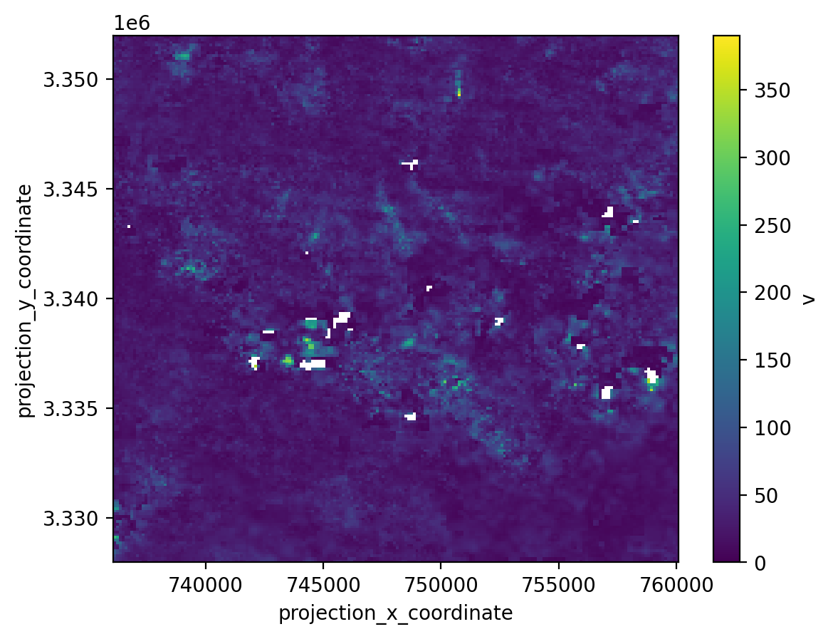
The above plot shows the mean of the magnitude of velocity variable along the time dimension. Note that you could plot the entire spatial extent of the data but it would take quite a bit of time. The rest of the notebooks in this chapter will demonstrate how to subset this spatially-large data object to specific areas of interest.
Conclusion#
This notebook demonstrated how to query and access zarr data cubes from the ITS_LIVE dataset. We also looked at reading data into python using
xarray, introducingdaskto our workflows, and some preliminary data visualization.The next notebook in the tutorial will take a look at the dataset in more detail and demonstrate ways to organize and manipulate data using
xarray.