3. Individual glacier data inspection#
This notebook will walk through steps to read in and organize velocity data and clip it to the extent of a single glacier. The tools we will use include xarray, rioxarray, geopandas, and flox.
To clip ITS_LIVE data to the extent of a single glacier, we will use a vector dataset of glacier outlines, the Randolph Glacier Inventory.
Learning goals#
Concepts#
Subset large raster dataset to area of interest using vector data
Examine different types of data stored within a raster object (in this example, the data is in the format of a zarr datacube
Handling different coordinate reference systems and projections
Dataset inspection using:
Xarray label- and index-based selection
Grouped computations and reductions
Visualization tools
Dimensional reductions and computations
Examining velocity component vectors
Calculating the magnitude of the displacement vector from velocity component vectors
Techniques#
Read in raster data using
xarrayRead in vector data using
geopandasManipulate and organize raster data using
xarrayfunctionalityExplore larger-than-memory data using
daskandxarrayTroubleshooting errors and warnings
Visualizing Xarray data using FacetGrid objects
Other useful resources#
These are resources that contain additional examples and discussion of the content in this notebook and more.
How do I… this is very helpful!
Xarray High-level computational patterns discussion of concepts and associated code examples
Parallel computing with dask Xarray tutorial demonstrating wrapping of dask arrays
Software + Setup#
First, let’s install the python libraries that we’ll need for this notebook:
%xmode minimal
Exception reporting mode: Minimal
import json
import os
import urllib.request
import cartopy
import geopandas as gpd
import matplotlib.pyplot as plt
import numpy as np
import pandas as pd
import rioxarray as rxr
import xarray as xr
from shapely.geometry import MultiPolygon, Point, Polygon
%config InlineBackend.figure_format='retina'
import logging
import psutil
from dask.distributed import Client, LocalCluster
#cluster = LocalCluster(
# n_workers = psutil.cpu_count(logical=True)-1,
# silence_logs = logging.ERROR,
# threads_per_worker=1,
#)
#client = Client(cluster)
#client
Reading in ITS_LIVE ice velocity dataset (raster data)#
We will use some of the functions we defined in the data access notebook in this notebook and others within this tutorial. They are all stored in the itslivetools.py file. If you cloned this tutorial from its github repository you’ll see that itslivetools.py is in the same directory as our current notebook, so we can import it with the following line:
import itslivetools
First, let’s read in the catalog again:
itslive_catalog = gpd.read_file('https://its-live-data.s3.amazonaws.com/datacubes/catalog_v02.json')
Next, we’ll use the gind_granule_by_point() and read_in_s3() functions to read in the ITS_LIVE zarr datacube as an xarray.Dataset object.
The read_in_s3() function will take a url that points to a zarr data cube stored in an AWS S3 bucket and return an xarray dataset.
I started with chunk_size='auto' which will choose chunk sizes that match the underlying data structure (this is generally ideal). More about choosing good chunk sizes here. If you want to use a different chunk size, specify it when you call the read_in_s3() function.
url = itslivetools.find_granule_by_point([95.180191, 30.645973])
url
'http://its-live-data.s3.amazonaws.com/datacubes/v2-updated-october2024/N30E090/ITS_LIVE_vel_EPSG32646_G0120_X750000_Y3350000.zarr'
dc = itslivetools.read_in_s3(url)
dc
<xarray.Dataset> Size: 1TB
Dimensions: (mid_date: 47892, y: 833, x: 833)
Coordinates:
* mid_date (mid_date) datetime64[ns] 383kB 2022-06-07T04...
* x (x) float64 7kB 7.001e+05 7.003e+05 ... 8e+05
* y (y) float64 7kB 3.4e+06 3.4e+06 ... 3.3e+06
Data variables: (12/60)
M11 (mid_date, y, x) float32 133GB dask.array<chunksize=(47892, 20, 20), meta=np.ndarray>
M11_dr_to_vr_factor (mid_date) float32 192kB dask.array<chunksize=(47892,), meta=np.ndarray>
M12 (mid_date, y, x) float32 133GB dask.array<chunksize=(47892, 20, 20), meta=np.ndarray>
M12_dr_to_vr_factor (mid_date) float32 192kB dask.array<chunksize=(47892,), meta=np.ndarray>
acquisition_date_img1 (mid_date) datetime64[ns] 383kB dask.array<chunksize=(47892,), meta=np.ndarray>
acquisition_date_img2 (mid_date) datetime64[ns] 383kB dask.array<chunksize=(47892,), meta=np.ndarray>
... ...
vy_error_modeled (mid_date) float32 192kB dask.array<chunksize=(47892,), meta=np.ndarray>
vy_error_slow (mid_date) float32 192kB dask.array<chunksize=(47892,), meta=np.ndarray>
vy_error_stationary (mid_date) float32 192kB dask.array<chunksize=(47892,), meta=np.ndarray>
vy_stable_shift (mid_date) float32 192kB dask.array<chunksize=(47892,), meta=np.ndarray>
vy_stable_shift_slow (mid_date) float32 192kB dask.array<chunksize=(47892,), meta=np.ndarray>
vy_stable_shift_stationary (mid_date) float32 192kB dask.array<chunksize=(47892,), meta=np.ndarray>
Attributes: (12/19)
Conventions: CF-1.8
GDAL_AREA_OR_POINT: Area
author: ITS_LIVE, a NASA MEaSUREs project (its-live.j...
autoRIFT_parameter_file: http://its-live-data.s3.amazonaws.com/autorif...
datacube_software_version: 1.0
date_created: 25-Sep-2023 22:00:23
... ...
s3: s3://its-live-data/datacubes/v2/N30E090/ITS_L...
skipped_granules: s3://its-live-data/datacubes/v2/N30E090/ITS_L...
time_standard_img1: UTC
time_standard_img2: UTC
title: ITS_LIVE datacube of image pair velocities
url: https://its-live-data.s3.amazonaws.com/datacu...- mid_date: 47892
- y: 833
- x: 833
- mid_date(mid_date)datetime64[ns]2022-06-07T04:21:44.211208960 .....
- description :
- midpoint of image 1 and image 2 acquisition date and time with granule's centroid longitude and latitude as microseconds
- standard_name :
- image_pair_center_date_with_time_separation
array(['2022-06-07T04:21:44.211208960', '2018-04-14T04:18:49.171219968', '2017-02-10T16:15:50.660901120', ..., '2024-01-23T04:18:19.231119104', '2023-06-01T04:10:44.893907968', '2023-09-02T16:18:20.230413056'], shape=(47892,), dtype='datetime64[ns]') - x(x)float647.001e+05 7.003e+05 ... 8e+05
- description :
- x coordinate of projection
- standard_name :
- projection_x_coordinate
array([700132.5, 700252.5, 700372.5, ..., 799732.5, 799852.5, 799972.5], shape=(833,)) - y(y)float643.4e+06 3.4e+06 ... 3.3e+06 3.3e+06
- description :
- y coordinate of projection
- standard_name :
- projection_y_coordinate
array([3399907.5, 3399787.5, 3399667.5, ..., 3300307.5, 3300187.5, 3300067.5], shape=(833,))
- M11(mid_date, y, x)float32dask.array<chunksize=(47892, 20, 20), meta=np.ndarray>
- description :
- conversion matrix element (1st row, 1st column) that can be multiplied with vx to give range pixel displacement dr (see Eq. A18 in https://www.mdpi.com/2072-4292/13/4/749)
- grid_mapping :
- mapping
- standard_name :
- conversion_matrix_element_11
- units :
- pixel/(meter/year)
Array Chunk Bytes 123.80 GiB 73.08 MiB Shape (47892, 833, 833) (47892, 20, 20) Dask graph 1764 chunks in 2 graph layers Data type float32 numpy.ndarray - M11_dr_to_vr_factor(mid_date)float32dask.array<chunksize=(47892,), meta=np.ndarray>
- description :
- multiplicative factor that converts slant range pixel displacement dr to slant range velocity vr
- standard_name :
- M11_dr_to_vr_factor
- units :
- meter/(year*pixel)
Array Chunk Bytes 187.08 kiB 187.08 kiB Shape (47892,) (47892,) Dask graph 1 chunks in 2 graph layers Data type float32 numpy.ndarray - M12(mid_date, y, x)float32dask.array<chunksize=(47892, 20, 20), meta=np.ndarray>
- description :
- conversion matrix element (1st row, 2nd column) that can be multiplied with vy to give range pixel displacement dr (see Eq. A18 in https://www.mdpi.com/2072-4292/13/4/749)
- grid_mapping :
- mapping
- standard_name :
- conversion_matrix_element_12
- units :
- pixel/(meter/year)
Array Chunk Bytes 123.80 GiB 73.08 MiB Shape (47892, 833, 833) (47892, 20, 20) Dask graph 1764 chunks in 2 graph layers Data type float32 numpy.ndarray - M12_dr_to_vr_factor(mid_date)float32dask.array<chunksize=(47892,), meta=np.ndarray>
- description :
- multiplicative factor that converts slant range pixel displacement dr to slant range velocity vr
- standard_name :
- M12_dr_to_vr_factor
- units :
- meter/(year*pixel)
Array Chunk Bytes 187.08 kiB 187.08 kiB Shape (47892,) (47892,) Dask graph 1 chunks in 2 graph layers Data type float32 numpy.ndarray - acquisition_date_img1(mid_date)datetime64[ns]dask.array<chunksize=(47892,), meta=np.ndarray>
- description :
- acquisition date and time of image 1
- standard_name :
- image1_acquition_date
Array Chunk Bytes 374.16 kiB 374.16 kiB Shape (47892,) (47892,) Dask graph 1 chunks in 2 graph layers Data type datetime64[ns] numpy.ndarray - acquisition_date_img2(mid_date)datetime64[ns]dask.array<chunksize=(47892,), meta=np.ndarray>
- description :
- acquisition date and time of image 2
- standard_name :
- image2_acquition_date
Array Chunk Bytes 374.16 kiB 374.16 kiB Shape (47892,) (47892,) Dask graph 1 chunks in 2 graph layers Data type datetime64[ns] numpy.ndarray - autoRIFT_software_version(mid_date)<U5dask.array<chunksize=(47892,), meta=np.ndarray>
- description :
- version of autoRIFT software
- standard_name :
- autoRIFT_software_version
Array Chunk Bytes 0.91 MiB 0.91 MiB Shape (47892,) (47892,) Dask graph 1 chunks in 2 graph layers Data type - chip_size_height(mid_date, y, x)float32dask.array<chunksize=(47892, 20, 20), meta=np.ndarray>
- chip_size_coordinates :
- Optical data: chip_size_coordinates = 'image projection geometry: width = x, height = y'. Radar data: chip_size_coordinates = 'radar geometry: width = range, height = azimuth'
- description :
- height of search template (chip)
- grid_mapping :
- mapping
- standard_name :
- chip_size_height
- units :
- m
- y_pixel_size :
- 10.0
Array Chunk Bytes 123.80 GiB 73.08 MiB Shape (47892, 833, 833) (47892, 20, 20) Dask graph 1764 chunks in 2 graph layers Data type float32 numpy.ndarray - chip_size_width(mid_date, y, x)float32dask.array<chunksize=(47892, 20, 20), meta=np.ndarray>
- chip_size_coordinates :
- Optical data: chip_size_coordinates = 'image projection geometry: width = x, height = y'. Radar data: chip_size_coordinates = 'radar geometry: width = range, height = azimuth'
- description :
- width of search template (chip)
- grid_mapping :
- mapping
- standard_name :
- chip_size_width
- units :
- m
- x_pixel_size :
- 10.0
Array Chunk Bytes 123.80 GiB 73.08 MiB Shape (47892, 833, 833) (47892, 20, 20) Dask graph 1764 chunks in 2 graph layers Data type float32 numpy.ndarray - date_center(mid_date)datetime64[ns]dask.array<chunksize=(47892,), meta=np.ndarray>
- description :
- midpoint of image 1 and image 2 acquisition date
- standard_name :
- image_pair_center_date
Array Chunk Bytes 374.16 kiB 374.16 kiB Shape (47892,) (47892,) Dask graph 1 chunks in 2 graph layers Data type datetime64[ns] numpy.ndarray - date_dt(mid_date)timedelta64[ns]dask.array<chunksize=(47892,), meta=np.ndarray>
- description :
- time separation between acquisition of image 1 and image 2
- standard_name :
- image_pair_time_separation
Array Chunk Bytes 374.16 kiB 374.16 kiB Shape (47892,) (47892,) Dask graph 1 chunks in 2 graph layers Data type timedelta64[ns] numpy.ndarray - floatingice(y, x)float32dask.array<chunksize=(833, 833), meta=np.ndarray>
- description :
- floating ice mask, 0 = non-floating-ice, 1 = floating-ice
- flag_meanings :
- non-ice ice
- flag_values :
- [0, 1]
- grid_mapping :
- mapping
- standard_name :
- floating ice mask
- url :
- https://its-live-data.s3.amazonaws.com/autorift_parameters/v001/N46_0120m_floatingice.tif
Array Chunk Bytes 2.65 MiB 2.65 MiB Shape (833, 833) (833, 833) Dask graph 1 chunks in 2 graph layers Data type float32 numpy.ndarray - granule_url(mid_date)<U1024dask.array<chunksize=(32736,), meta=np.ndarray>
- description :
- original granule URL
- standard_name :
- granule_url
Array Chunk Bytes 187.08 MiB 127.88 MiB Shape (47892,) (32736,) Dask graph 2 chunks in 2 graph layers Data type - interp_mask(mid_date, y, x)float32dask.array<chunksize=(47892, 20, 20), meta=np.ndarray>
- description :
- light interpolation mask
- flag_meanings :
- measured interpolated
- flag_values :
- [0, 1]
- grid_mapping :
- mapping
- standard_name :
- interpolated_value_mask
Array Chunk Bytes 123.80 GiB 73.08 MiB Shape (47892, 833, 833) (47892, 20, 20) Dask graph 1764 chunks in 2 graph layers Data type float32 numpy.ndarray - landice(y, x)float32dask.array<chunksize=(833, 833), meta=np.ndarray>
- description :
- land ice mask, 0 = non-land-ice, 1 = land-ice
- flag_meanings :
- non-ice ice
- flag_values :
- [0, 1]
- grid_mapping :
- mapping
- standard_name :
- land ice mask
- url :
- https://its-live-data.s3.amazonaws.com/autorift_parameters/v001/N46_0120m_landice.tif
Array Chunk Bytes 2.65 MiB 2.65 MiB Shape (833, 833) (833, 833) Dask graph 1 chunks in 2 graph layers Data type float32 numpy.ndarray - mapping()<U1...
- GeoTransform :
- 700072.5 120.0 0 3399967.5 0 -120.0
- crs_wkt :
- PROJCS["WGS 84 / UTM zone 46N",GEOGCS["WGS 84",DATUM["WGS_1984",SPHEROID["WGS 84",6378137,298.257223563,AUTHORITY["EPSG","7030"]],AUTHORITY["EPSG","6326"]],PRIMEM["Greenwich",0,AUTHORITY["EPSG","8901"]],UNIT["degree",0.0174532925199433,AUTHORITY["EPSG","9122"]],AUTHORITY["EPSG","4326"]],PROJECTION["Transverse_Mercator"],PARAMETER["latitude_of_origin",0],PARAMETER["central_meridian",93],PARAMETER["scale_factor",0.9996],PARAMETER["false_easting",500000],PARAMETER["false_northing",0],UNIT["metre",1,AUTHORITY["EPSG","9001"]],AXIS["Easting",EAST],AXIS["Northing",NORTH],AUTHORITY["EPSG","32646"]]
- false_easting :
- 500000.0
- false_northing :
- 0.0
- grid_mapping_name :
- universal_transverse_mercator
- inverse_flattening :
- 298.257223563
- latitude_of_projection_origin :
- 0.0
- longitude_of_central_meridian :
- 93.0
- proj4text :
- +proj=utm +zone=46 +datum=WGS84 +units=m +no_defs
- scale_factor_at_central_meridian :
- 0.9996
- semi_major_axis :
- 6378137.0
- spatial_epsg :
- 32646
- spatial_ref :
- PROJCS["WGS 84 / UTM zone 46N",GEOGCS["WGS 84",DATUM["WGS_1984",SPHEROID["WGS 84",6378137,298.257223563,AUTHORITY["EPSG","7030"]],AUTHORITY["EPSG","6326"]],PRIMEM["Greenwich",0,AUTHORITY["EPSG","8901"]],UNIT["degree",0.0174532925199433,AUTHORITY["EPSG","9122"]],AUTHORITY["EPSG","4326"]],PROJECTION["Transverse_Mercator"],PARAMETER["latitude_of_origin",0],PARAMETER["central_meridian",93],PARAMETER["scale_factor",0.9996],PARAMETER["false_easting",500000],PARAMETER["false_northing",0],UNIT["metre",1,AUTHORITY["EPSG","9001"]],AXIS["Easting",EAST],AXIS["Northing",NORTH],AUTHORITY["EPSG","32646"]]
- utm_zone_number :
- 46.0
[1 values with dtype=<U1]
- mission_img1(mid_date)<U1dask.array<chunksize=(47892,), meta=np.ndarray>
- description :
- id of the mission that acquired image 1
- standard_name :
- image1_mission
Array Chunk Bytes 187.08 kiB 187.08 kiB Shape (47892,) (47892,) Dask graph 1 chunks in 2 graph layers Data type - mission_img2(mid_date)<U1dask.array<chunksize=(47892,), meta=np.ndarray>
- description :
- id of the mission that acquired image 2
- standard_name :
- image2_mission
Array Chunk Bytes 187.08 kiB 187.08 kiB Shape (47892,) (47892,) Dask graph 1 chunks in 2 graph layers Data type - roi_valid_percentage(mid_date)float32dask.array<chunksize=(47892,), meta=np.ndarray>
- description :
- percentage of pixels with a valid velocity estimate determined for the intersection of the full image pair footprint and the region of interest (roi) that defines where autoRIFT tried to estimate a velocity
- standard_name :
- region_of_interest_valid_pixel_percentage
Array Chunk Bytes 187.08 kiB 187.08 kiB Shape (47892,) (47892,) Dask graph 1 chunks in 2 graph layers Data type float32 numpy.ndarray - satellite_img1(mid_date)<U2dask.array<chunksize=(47892,), meta=np.ndarray>
- description :
- id of the satellite that acquired image 1
- standard_name :
- image1_satellite
Array Chunk Bytes 374.16 kiB 374.16 kiB Shape (47892,) (47892,) Dask graph 1 chunks in 2 graph layers Data type - satellite_img2(mid_date)<U2dask.array<chunksize=(47892,), meta=np.ndarray>
- description :
- id of the satellite that acquired image 2
- standard_name :
- image2_satellite
Array Chunk Bytes 374.16 kiB 374.16 kiB Shape (47892,) (47892,) Dask graph 1 chunks in 2 graph layers Data type - sensor_img1(mid_date)<U3dask.array<chunksize=(47892,), meta=np.ndarray>
- description :
- id of the sensor that acquired image 1
- standard_name :
- image1_sensor
Array Chunk Bytes 561.23 kiB 561.23 kiB Shape (47892,) (47892,) Dask graph 1 chunks in 2 graph layers Data type - sensor_img2(mid_date)<U3dask.array<chunksize=(47892,), meta=np.ndarray>
- description :
- id of the sensor that acquired image 2
- standard_name :
- image2_sensor
Array Chunk Bytes 561.23 kiB 561.23 kiB Shape (47892,) (47892,) Dask graph 1 chunks in 2 graph layers Data type - stable_count_slow(mid_date)uint16dask.array<chunksize=(47892,), meta=np.ndarray>
- description :
- number of valid pixels over slowest 25% of ice
- standard_name :
- stable_count_slow
- units :
- count
Array Chunk Bytes 93.54 kiB 93.54 kiB Shape (47892,) (47892,) Dask graph 1 chunks in 2 graph layers Data type uint16 numpy.ndarray - stable_count_stationary(mid_date)uint16dask.array<chunksize=(47892,), meta=np.ndarray>
- description :
- number of valid pixels over stationary or slow-flowing surfaces
- standard_name :
- stable_count_stationary
- units :
- count
Array Chunk Bytes 93.54 kiB 93.54 kiB Shape (47892,) (47892,) Dask graph 1 chunks in 2 graph layers Data type uint16 numpy.ndarray - stable_shift_flag(mid_date)uint8dask.array<chunksize=(47892,), meta=np.ndarray>
- description :
- flag for applying velocity bias correction: 0 = no correction; 1 = correction from overlapping stable surface mask (stationary or slow-flowing surfaces with velocity < 15 m/yr)(top priority); 2 = correction from slowest 25% of overlapping velocities (second priority)
- standard_name :
- stable_shift_flag
Array Chunk Bytes 46.77 kiB 46.77 kiB Shape (47892,) (47892,) Dask graph 1 chunks in 2 graph layers Data type uint8 numpy.ndarray - v(mid_date, y, x)float32dask.array<chunksize=(47892, 20, 20), meta=np.ndarray>
- description :
- velocity magnitude
- grid_mapping :
- mapping
- standard_name :
- land_ice_surface_velocity
- units :
- meter/year
Array Chunk Bytes 123.80 GiB 73.08 MiB Shape (47892, 833, 833) (47892, 20, 20) Dask graph 1764 chunks in 2 graph layers Data type float32 numpy.ndarray - v_error(mid_date, y, x)float32dask.array<chunksize=(47892, 20, 20), meta=np.ndarray>
- description :
- velocity magnitude error
- grid_mapping :
- mapping
- standard_name :
- velocity_error
- units :
- meter/year
Array Chunk Bytes 123.80 GiB 73.08 MiB Shape (47892, 833, 833) (47892, 20, 20) Dask graph 1764 chunks in 2 graph layers Data type float32 numpy.ndarray - va(mid_date, y, x)float32dask.array<chunksize=(47892, 20, 20), meta=np.ndarray>
- description :
- velocity in radar azimuth direction
- grid_mapping :
- mapping
Array Chunk Bytes 123.80 GiB 73.08 MiB Shape (47892, 833, 833) (47892, 20, 20) Dask graph 1764 chunks in 2 graph layers Data type float32 numpy.ndarray - va_error(mid_date)float32dask.array<chunksize=(47892,), meta=np.ndarray>
- description :
- error for velocity in radar azimuth direction
- standard_name :
- va_error
- units :
- meter/year
Array Chunk Bytes 187.08 kiB 187.08 kiB Shape (47892,) (47892,) Dask graph 1 chunks in 2 graph layers Data type float32 numpy.ndarray - va_error_modeled(mid_date)float32dask.array<chunksize=(47892,), meta=np.ndarray>
- description :
- 1-sigma error calculated using a modeled error-dt relationship
- standard_name :
- va_error_modeled
- units :
- meter/year
Array Chunk Bytes 187.08 kiB 187.08 kiB Shape (47892,) (47892,) Dask graph 1 chunks in 2 graph layers Data type float32 numpy.ndarray - va_error_slow(mid_date)float32dask.array<chunksize=(47892,), meta=np.ndarray>
- description :
- RMSE over slowest 25% of retrieved velocities
- standard_name :
- va_error_slow
- units :
- meter/year
Array Chunk Bytes 187.08 kiB 187.08 kiB Shape (47892,) (47892,) Dask graph 1 chunks in 2 graph layers Data type float32 numpy.ndarray - va_error_stationary(mid_date)float32dask.array<chunksize=(47892,), meta=np.ndarray>
- description :
- RMSE over stable surfaces, stationary or slow-flowing surfaces with velocity < 15 m/yr identified from an external mask
- standard_name :
- va_error_stationary
- units :
- meter/year
Array Chunk Bytes 187.08 kiB 187.08 kiB Shape (47892,) (47892,) Dask graph 1 chunks in 2 graph layers Data type float32 numpy.ndarray - va_stable_shift(mid_date)float32dask.array<chunksize=(47892,), meta=np.ndarray>
- description :
- applied va shift calibrated using pixels over stable or slow surfaces
- standard_name :
- va_stable_shift
- units :
- meter/year
Array Chunk Bytes 187.08 kiB 187.08 kiB Shape (47892,) (47892,) Dask graph 1 chunks in 2 graph layers Data type float32 numpy.ndarray - va_stable_shift_slow(mid_date)float32dask.array<chunksize=(47892,), meta=np.ndarray>
- description :
- va shift calibrated using valid pixels over slowest 25% of retrieved velocities
- standard_name :
- va_stable_shift_slow
- units :
- meter/year
Array Chunk Bytes 187.08 kiB 187.08 kiB Shape (47892,) (47892,) Dask graph 1 chunks in 2 graph layers Data type float32 numpy.ndarray - va_stable_shift_stationary(mid_date)float32dask.array<chunksize=(47892,), meta=np.ndarray>
- description :
- va shift calibrated using valid pixels over stable surfaces, stationary or slow-flowing surfaces with velocity < 15 m/yr identified from an external mask
- standard_name :
- va_stable_shift_stationary
- units :
- meter/year
Array Chunk Bytes 187.08 kiB 187.08 kiB Shape (47892,) (47892,) Dask graph 1 chunks in 2 graph layers Data type float32 numpy.ndarray - vr(mid_date, y, x)float32dask.array<chunksize=(47892, 20, 20), meta=np.ndarray>
- description :
- velocity in radar range direction
- grid_mapping :
- mapping
Array Chunk Bytes 123.80 GiB 73.08 MiB Shape (47892, 833, 833) (47892, 20, 20) Dask graph 1764 chunks in 2 graph layers Data type float32 numpy.ndarray - vr_error(mid_date)float32dask.array<chunksize=(47892,), meta=np.ndarray>
- description :
- error for velocity in radar range direction
- standard_name :
- vr_error
- units :
- meter/year
Array Chunk Bytes 187.08 kiB 187.08 kiB Shape (47892,) (47892,) Dask graph 1 chunks in 2 graph layers Data type float32 numpy.ndarray - vr_error_modeled(mid_date)float32dask.array<chunksize=(47892,), meta=np.ndarray>
- description :
- 1-sigma error calculated using a modeled error-dt relationship
- standard_name :
- vr_error_modeled
- units :
- meter/year
Array Chunk Bytes 187.08 kiB 187.08 kiB Shape (47892,) (47892,) Dask graph 1 chunks in 2 graph layers Data type float32 numpy.ndarray - vr_error_slow(mid_date)float32dask.array<chunksize=(47892,), meta=np.ndarray>
- description :
- RMSE over slowest 25% of retrieved velocities
- standard_name :
- vr_error_slow
- units :
- meter/year
Array Chunk Bytes 187.08 kiB 187.08 kiB Shape (47892,) (47892,) Dask graph 1 chunks in 2 graph layers Data type float32 numpy.ndarray - vr_error_stationary(mid_date)float32dask.array<chunksize=(47892,), meta=np.ndarray>
- description :
- RMSE over stable surfaces, stationary or slow-flowing surfaces with velocity < 15 m/yr identified from an external mask
- standard_name :
- vr_error_stationary
- units :
- meter/year
Array Chunk Bytes 187.08 kiB 187.08 kiB Shape (47892,) (47892,) Dask graph 1 chunks in 2 graph layers Data type float32 numpy.ndarray - vr_stable_shift(mid_date)float32dask.array<chunksize=(47892,), meta=np.ndarray>
- description :
- applied vr shift calibrated using pixels over stable or slow surfaces
- standard_name :
- vr_stable_shift
- units :
- meter/year
Array Chunk Bytes 187.08 kiB 187.08 kiB Shape (47892,) (47892,) Dask graph 1 chunks in 2 graph layers Data type float32 numpy.ndarray - vr_stable_shift_slow(mid_date)float32dask.array<chunksize=(47892,), meta=np.ndarray>
- description :
- vr shift calibrated using valid pixels over slowest 25% of retrieved velocities
- standard_name :
- vr_stable_shift_slow
- units :
- meter/year
Array Chunk Bytes 187.08 kiB 187.08 kiB Shape (47892,) (47892,) Dask graph 1 chunks in 2 graph layers Data type float32 numpy.ndarray - vr_stable_shift_stationary(mid_date)float32dask.array<chunksize=(47892,), meta=np.ndarray>
- description :
- vr shift calibrated using valid pixels over stable surfaces, stationary or slow-flowing surfaces with velocity < 15 m/yr identified from an external mask
- standard_name :
- vr_stable_shift_stationary
- units :
- meter/year
Array Chunk Bytes 187.08 kiB 187.08 kiB Shape (47892,) (47892,) Dask graph 1 chunks in 2 graph layers Data type float32 numpy.ndarray - vx(mid_date, y, x)float32dask.array<chunksize=(47892, 20, 20), meta=np.ndarray>
- description :
- velocity component in x direction
- grid_mapping :
- mapping
- standard_name :
- land_ice_surface_x_velocity
- units :
- meter/year
Array Chunk Bytes 123.80 GiB 73.08 MiB Shape (47892, 833, 833) (47892, 20, 20) Dask graph 1764 chunks in 2 graph layers Data type float32 numpy.ndarray - vx_error(mid_date)float32dask.array<chunksize=(47892,), meta=np.ndarray>
- description :
- best estimate of x_velocity error: vx_error is populated according to the approach used for the velocity bias correction as indicated in "stable_shift_flag"
- standard_name :
- vx_error
- units :
- meter/year
Array Chunk Bytes 187.08 kiB 187.08 kiB Shape (47892,) (47892,) Dask graph 1 chunks in 2 graph layers Data type float32 numpy.ndarray - vx_error_modeled(mid_date)float32dask.array<chunksize=(47892,), meta=np.ndarray>
- description :
- 1-sigma error calculated using a modeled error-dt relationship
- standard_name :
- vx_error_modeled
- units :
- meter/year
Array Chunk Bytes 187.08 kiB 187.08 kiB Shape (47892,) (47892,) Dask graph 1 chunks in 2 graph layers Data type float32 numpy.ndarray - vx_error_slow(mid_date)float32dask.array<chunksize=(47892,), meta=np.ndarray>
- description :
- RMSE over slowest 25% of retrieved velocities
- standard_name :
- vx_error_slow
- units :
- meter/year
Array Chunk Bytes 187.08 kiB 187.08 kiB Shape (47892,) (47892,) Dask graph 1 chunks in 2 graph layers Data type float32 numpy.ndarray - vx_error_stationary(mid_date)float32dask.array<chunksize=(47892,), meta=np.ndarray>
- description :
- RMSE over stable surfaces, stationary or slow-flowing surfaces with velocity < 15 meter/year identified from an external mask
- standard_name :
- vx_error_stationary
- units :
- meter/year
Array Chunk Bytes 187.08 kiB 187.08 kiB Shape (47892,) (47892,) Dask graph 1 chunks in 2 graph layers Data type float32 numpy.ndarray - vx_stable_shift(mid_date)float32dask.array<chunksize=(47892,), meta=np.ndarray>
- description :
- applied vx shift calibrated using pixels over stable or slow surfaces
- standard_name :
- vx_stable_shift
- units :
- meter/year
Array Chunk Bytes 187.08 kiB 187.08 kiB Shape (47892,) (47892,) Dask graph 1 chunks in 2 graph layers Data type float32 numpy.ndarray - vx_stable_shift_slow(mid_date)float32dask.array<chunksize=(47892,), meta=np.ndarray>
- description :
- vx shift calibrated using valid pixels over slowest 25% of retrieved velocities
- standard_name :
- vx_stable_shift_slow
- units :
- meter/year
Array Chunk Bytes 187.08 kiB 187.08 kiB Shape (47892,) (47892,) Dask graph 1 chunks in 2 graph layers Data type float32 numpy.ndarray - vx_stable_shift_stationary(mid_date)float32dask.array<chunksize=(47892,), meta=np.ndarray>
- description :
- vx shift calibrated using valid pixels over stable surfaces, stationary or slow-flowing surfaces with velocity < 15 m/yr identified from an external mask
- standard_name :
- vx_stable_shift_stationary
- units :
- meter/year
Array Chunk Bytes 187.08 kiB 187.08 kiB Shape (47892,) (47892,) Dask graph 1 chunks in 2 graph layers Data type float32 numpy.ndarray - vy(mid_date, y, x)float32dask.array<chunksize=(47892, 20, 20), meta=np.ndarray>
- description :
- velocity component in y direction
- grid_mapping :
- mapping
- standard_name :
- land_ice_surface_y_velocity
- units :
- meter/year
Array Chunk Bytes 123.80 GiB 73.08 MiB Shape (47892, 833, 833) (47892, 20, 20) Dask graph 1764 chunks in 2 graph layers Data type float32 numpy.ndarray - vy_error(mid_date)float32dask.array<chunksize=(47892,), meta=np.ndarray>
- description :
- best estimate of y_velocity error: vy_error is populated according to the approach used for the velocity bias correction as indicated in "stable_shift_flag"
- standard_name :
- vy_error
- units :
- meter/year
Array Chunk Bytes 187.08 kiB 187.08 kiB Shape (47892,) (47892,) Dask graph 1 chunks in 2 graph layers Data type float32 numpy.ndarray - vy_error_modeled(mid_date)float32dask.array<chunksize=(47892,), meta=np.ndarray>
- description :
- 1-sigma error calculated using a modeled error-dt relationship
- standard_name :
- vy_error_modeled
- units :
- meter/year
Array Chunk Bytes 187.08 kiB 187.08 kiB Shape (47892,) (47892,) Dask graph 1 chunks in 2 graph layers Data type float32 numpy.ndarray - vy_error_slow(mid_date)float32dask.array<chunksize=(47892,), meta=np.ndarray>
- description :
- RMSE over slowest 25% of retrieved velocities
- standard_name :
- vy_error_slow
- units :
- meter/year
Array Chunk Bytes 187.08 kiB 187.08 kiB Shape (47892,) (47892,) Dask graph 1 chunks in 2 graph layers Data type float32 numpy.ndarray - vy_error_stationary(mid_date)float32dask.array<chunksize=(47892,), meta=np.ndarray>
- description :
- RMSE over stable surfaces, stationary or slow-flowing surfaces with velocity < 15 meter/year identified from an external mask
- standard_name :
- vy_error_stationary
- units :
- meter/year
Array Chunk Bytes 187.08 kiB 187.08 kiB Shape (47892,) (47892,) Dask graph 1 chunks in 2 graph layers Data type float32 numpy.ndarray - vy_stable_shift(mid_date)float32dask.array<chunksize=(47892,), meta=np.ndarray>
- description :
- applied vy shift calibrated using pixels over stable or slow surfaces
- standard_name :
- vy_stable_shift
- units :
- meter/year
Array Chunk Bytes 187.08 kiB 187.08 kiB Shape (47892,) (47892,) Dask graph 1 chunks in 2 graph layers Data type float32 numpy.ndarray - vy_stable_shift_slow(mid_date)float32dask.array<chunksize=(47892,), meta=np.ndarray>
- description :
- vy shift calibrated using valid pixels over slowest 25% of retrieved velocities
- standard_name :
- vy_stable_shift_slow
- units :
- meter/year
Array Chunk Bytes 187.08 kiB 187.08 kiB Shape (47892,) (47892,) Dask graph 1 chunks in 2 graph layers Data type float32 numpy.ndarray - vy_stable_shift_stationary(mid_date)float32dask.array<chunksize=(47892,), meta=np.ndarray>
- description :
- vy shift calibrated using valid pixels over stable surfaces, stationary or slow-flowing surfaces with velocity < 15 m/yr identified from an external mask
- standard_name :
- vy_stable_shift_stationary
- units :
- meter/year
Array Chunk Bytes 187.08 kiB 187.08 kiB Shape (47892,) (47892,) Dask graph 1 chunks in 2 graph layers Data type float32 numpy.ndarray
- mid_datePandasIndex
PandasIndex(DatetimeIndex(['2022-06-07 04:21:44.211208960', '2018-04-14 04:18:49.171219968', '2017-02-10 16:15:50.660901120', '2022-04-03 04:19:01.211214080', '2021-07-22 04:16:46.210427904', '2019-03-15 04:15:44.180925952', '2002-09-15 03:59:12.379172096', '2002-12-28 03:42:16.181281024', '2021-06-29 16:16:10.210323968', '2022-03-26 16:18:35.211123968', ... '2021-10-05 04:15:51.210407936', '2022-11-11 16:15:55.220602112', '2022-06-29 16:19:50.211113984', '2023-08-18 16:18:10.230522880', '2023-08-03 16:18:00.221108992', '2022-12-16 16:16:00.220919808', '2023-02-12 04:15:56.220721920', '2024-01-23 04:18:19.231119104', '2023-06-01 04:10:44.893907968', '2023-09-02 16:18:20.230413056'], dtype='datetime64[ns]', name='mid_date', length=47892, freq=None)) - xPandasIndex
PandasIndex(Index([700132.5, 700252.5, 700372.5, 700492.5, 700612.5, 700732.5, 700852.5, 700972.5, 701092.5, 701212.5, ... 798892.5, 799012.5, 799132.5, 799252.5, 799372.5, 799492.5, 799612.5, 799732.5, 799852.5, 799972.5], dtype='float64', name='x', length=833)) - yPandasIndex
PandasIndex(Index([3399907.5, 3399787.5, 3399667.5, 3399547.5, 3399427.5, 3399307.5, 3399187.5, 3399067.5, 3398947.5, 3398827.5, ... 3301147.5, 3301027.5, 3300907.5, 3300787.5, 3300667.5, 3300547.5, 3300427.5, 3300307.5, 3300187.5, 3300067.5], dtype='float64', name='y', length=833))
- Conventions :
- CF-1.8
- GDAL_AREA_OR_POINT :
- Area
- author :
- ITS_LIVE, a NASA MEaSUREs project (its-live.jpl.nasa.gov)
- autoRIFT_parameter_file :
- http://its-live-data.s3.amazonaws.com/autorift_parameters/v001/autorift_landice_0120m.shp
- datacube_software_version :
- 1.0
- date_created :
- 25-Sep-2023 22:00:23
- date_updated :
- 13-Nov-2024 00:08:07
- geo_polygon :
- [[95.06959008486952, 29.814255053135895], [95.32812062059084, 29.809951334550703], [95.58659184122865, 29.80514261876954], [95.84499718862224, 29.7998293459177], [96.10333011481168, 29.79401200205343], [96.11032804508507, 30.019297601073085], [96.11740568350054, 30.244573983323825], [96.12456379063154, 30.469841094022847], [96.1318031397002, 30.695098878594504], [95.87110827645229, 30.70112924501256], [95.61033817656023, 30.7066371044805], [95.34949964126946, 30.711621947056347], [95.08859948278467, 30.716083310981194], [95.08376623410525, 30.49063893600811], [95.07898726183609, 30.26518607254204], [95.0742620484426, 30.039724763743482], [95.06959008486952, 29.814255053135895]]
- institution :
- NASA Jet Propulsion Laboratory (JPL), California Institute of Technology
- latitude :
- 30.26
- longitude :
- 95.6
- proj_polygon :
- [[700000, 3300000], [725000.0, 3300000.0], [750000.0, 3300000.0], [775000.0, 3300000.0], [800000, 3300000], [800000.0, 3325000.0], [800000.0, 3350000.0], [800000.0, 3375000.0], [800000, 3400000], [775000.0, 3400000.0], [750000.0, 3400000.0], [725000.0, 3400000.0], [700000, 3400000], [700000.0, 3375000.0], [700000.0, 3350000.0], [700000.0, 3325000.0], [700000, 3300000]]
- projection :
- 32646
- s3 :
- s3://its-live-data/datacubes/v2/N30E090/ITS_LIVE_vel_EPSG32646_G0120_X750000_Y3350000.zarr
- skipped_granules :
- s3://its-live-data/datacubes/v2/N30E090/ITS_LIVE_vel_EPSG32646_G0120_X750000_Y3350000.json
- time_standard_img1 :
- UTC
- time_standard_img2 :
- UTC
- title :
- ITS_LIVE datacube of image pair velocities
- url :
- https://its-live-data.s3.amazonaws.com/datacubes/v2/N30E090/ITS_LIVE_vel_EPSG32646_G0120_X750000_Y3350000.zarr
Working with dask#
We can see that this is a very large dataset. We have a time dimension with a length of 25,243, and then x and y dimensions that are both 833 units long. There are 60 variables within this dataset that exist along some or all of the dimensions (with the exception of the mapping data variable which contains geographic information. If you expand one of the 3-dimensional variables (exists along x,y, and mid_date) you’ll see that it is very large (65 GB!). This is more than my computer can handle so we will use dask, which is a python package for parallelizing and scaling workflows that let’s us work with larger-than-memory data efficiently.
dc.v
<xarray.DataArray 'v' (mid_date: 47892, y: 833, x: 833)> Size: 133GB
dask.array<open_dataset-v, shape=(47892, 833, 833), dtype=float32, chunksize=(47892, 20, 20), chunktype=numpy.ndarray>
Coordinates:
* mid_date (mid_date) datetime64[ns] 383kB 2022-06-07T04:21:44.211208960 ....
* x (x) float64 7kB 7.001e+05 7.003e+05 7.004e+05 ... 7.999e+05 8e+05
* y (y) float64 7kB 3.4e+06 3.4e+06 3.4e+06 ... 3.3e+06 3.3e+06
Attributes:
description: velocity magnitude
grid_mapping: mapping
standard_name: land_ice_surface_velocity
units: meter/year- mid_date: 47892
- y: 833
- x: 833
- dask.array<chunksize=(47892, 20, 20), meta=np.ndarray>
Array Chunk Bytes 123.80 GiB 73.08 MiB Shape (47892, 833, 833) (47892, 20, 20) Dask graph 1764 chunks in 2 graph layers Data type float32 numpy.ndarray - mid_date(mid_date)datetime64[ns]2022-06-07T04:21:44.211208960 .....
- description :
- midpoint of image 1 and image 2 acquisition date and time with granule's centroid longitude and latitude as microseconds
- standard_name :
- image_pair_center_date_with_time_separation
array(['2022-06-07T04:21:44.211208960', '2018-04-14T04:18:49.171219968', '2017-02-10T16:15:50.660901120', ..., '2024-01-23T04:18:19.231119104', '2023-06-01T04:10:44.893907968', '2023-09-02T16:18:20.230413056'], shape=(47892,), dtype='datetime64[ns]') - x(x)float647.001e+05 7.003e+05 ... 8e+05
- description :
- x coordinate of projection
- standard_name :
- projection_x_coordinate
array([700132.5, 700252.5, 700372.5, ..., 799732.5, 799852.5, 799972.5], shape=(833,)) - y(y)float643.4e+06 3.4e+06 ... 3.3e+06 3.3e+06
- description :
- y coordinate of projection
- standard_name :
- projection_y_coordinate
array([3399907.5, 3399787.5, 3399667.5, ..., 3300307.5, 3300187.5, 3300067.5], shape=(833,))
- mid_datePandasIndex
PandasIndex(DatetimeIndex(['2022-06-07 04:21:44.211208960', '2018-04-14 04:18:49.171219968', '2017-02-10 16:15:50.660901120', '2022-04-03 04:19:01.211214080', '2021-07-22 04:16:46.210427904', '2019-03-15 04:15:44.180925952', '2002-09-15 03:59:12.379172096', '2002-12-28 03:42:16.181281024', '2021-06-29 16:16:10.210323968', '2022-03-26 16:18:35.211123968', ... '2021-10-05 04:15:51.210407936', '2022-11-11 16:15:55.220602112', '2022-06-29 16:19:50.211113984', '2023-08-18 16:18:10.230522880', '2023-08-03 16:18:00.221108992', '2022-12-16 16:16:00.220919808', '2023-02-12 04:15:56.220721920', '2024-01-23 04:18:19.231119104', '2023-06-01 04:10:44.893907968', '2023-09-02 16:18:20.230413056'], dtype='datetime64[ns]', name='mid_date', length=47892, freq=None)) - xPandasIndex
PandasIndex(Index([700132.5, 700252.5, 700372.5, 700492.5, 700612.5, 700732.5, 700852.5, 700972.5, 701092.5, 701212.5, ... 798892.5, 799012.5, 799132.5, 799252.5, 799372.5, 799492.5, 799612.5, 799732.5, 799852.5, 799972.5], dtype='float64', name='x', length=833)) - yPandasIndex
PandasIndex(Index([3399907.5, 3399787.5, 3399667.5, 3399547.5, 3399427.5, 3399307.5, 3399187.5, 3399067.5, 3398947.5, 3398827.5, ... 3301147.5, 3301027.5, 3300907.5, 3300787.5, 3300667.5, 3300547.5, 3300427.5, 3300307.5, 3300187.5, 3300067.5], dtype='float64', name='y', length=833))
- description :
- velocity magnitude
- grid_mapping :
- mapping
- standard_name :
- land_ice_surface_velocity
- units :
- meter/year
We are reading this in as a dask array. Let’s take a look at the chunk sizes:
Note
chunksizes shows the largest chunk size. chunks shows the sizes of all chunks along all dims, better if you have irregular chunks
dc.chunksizes
ValueError: Object has inconsistent chunks along dimension y. This can be fixed by calling unify_chunks().
As suggested in the error message, apply the unify_chunks() method:
dc = dc.unify_chunks()
Great, that worked. Now we can see the chunk sizes of the dataset:
dc.chunksizes
Frozen({'mid_date': (32736, 15156), 'y': (20, 20, 20, 20, 20, 20, 20, 20, 20, 20, 20, 20, 20, 20, 20, 20, 20, 20, 20, 20, 20, 20, 20, 20, 20, 20, 20, 20, 20, 20, 20, 20, 20, 20, 20, 20, 20, 20, 20, 20, 20, 13), 'x': (20, 20, 20, 20, 20, 20, 20, 20, 20, 20, 20, 20, 20, 20, 20, 20, 20, 20, 20, 20, 20, 20, 20, 20, 20, 20, 20, 20, 20, 20, 20, 20, 20, 20, 20, 20, 20, 20, 20, 20, 20, 13)})
Note
Setting the dask chunksize to auto at the xr.open_dataset() step will use chunk sizes that most closely resemble the structure of the underlying data. To avoid imposing a chunk size that isn’t a good fit for the data, avoid re-chunking until we have selected a subset of our area of interest from the larger dataset
Check CRS of xr object:
dc.attrs['projection']
'32646'
Let’s take a look at the time dimension (mid_date here). To start with we’ll just print the first 10 values:
for element in range(10):
print(dc.mid_date[element].data)
2022-06-07T04:21:44.211208960
2018-04-14T04:18:49.171219968
2017-02-10T16:15:50.660901120
2022-04-03T04:19:01.211214080
2021-07-22T04:16:46.210427904
2019-03-15T04:15:44.180925952
2002-09-15T03:59:12.379172096
2002-12-28T03:42:16.181281024
2021-06-29T16:16:10.210323968
2022-03-26T16:18:35.211123968
It doesn’t look like the time dimension is in chronological order, let’s fix that:
Note
The following cell is commented out because it produces an error and usually leads to a dead kernel. Let’s try to troubleshoot this below. {add image of error (in screenshots)}
dc_timesorted = dc.sortby(dc['mid_date'])
Note: work-around for situation where above cell produces error#
Note
In some test cases, the above cell triggered the following error. While the current version runs fine, I’m including a work around in the following cells in case you encounter this error as well. If you don’t, feel free to skip ahead to the next sub-section heading{add image of error (in screenshots)}
Let’s follow some internet advice and try to fix this issue. We will actually start over from the very beginning and read in the dataset using only xarray and not dask.
dc_new = xr.open_dataset(url, engine='zarr')
Now we have an xr.Dataset that is built on numpy arrays rather than dask arrays, which means we can re-index along the time dimension using xarray’s ‘lazy’ functionality:
dc_new_timesorted = dc_new.sortby(dc_new['mid_date'])
for element in range(10):
print(dc_new_timesorted.mid_date[element].data)
1986-09-11T03:31:15.003252992
1986-10-05T03:31:06.144750016
1986-10-21T03:31:34.493249984
1986-11-22T03:29:27.023556992
1986-11-30T03:29:08.710132992
1986-12-08T03:29:55.372057024
1986-12-08T03:33:17.095283968
1986-12-16T03:30:10.645544000
1986-12-24T03:29:52.332120960
1987-01-09T03:30:01.787228992
Great, much easier. Now, we will chunk the dataset.
dc_new_timesorted = dc_new_timesorted.chunk()
dc_new_timesorted.chunks
Frozen({'mid_date': (47892,), 'y': (833,), 'x': (833,)})
dc_new_timesorted
<xarray.Dataset> Size: 1TB
Dimensions: (mid_date: 47892, y: 833, x: 833)
Coordinates:
* mid_date (mid_date) datetime64[ns] 383kB 1986-09-11T03...
* x (x) float64 7kB 7.001e+05 7.003e+05 ... 8e+05
* y (y) float64 7kB 3.4e+06 3.4e+06 ... 3.3e+06
Data variables: (12/60)
M11 (mid_date, y, x) float32 133GB dask.array<chunksize=(47892, 833, 833), meta=np.ndarray>
M11_dr_to_vr_factor (mid_date) float32 192kB dask.array<chunksize=(47892,), meta=np.ndarray>
M12 (mid_date, y, x) float32 133GB dask.array<chunksize=(47892, 833, 833), meta=np.ndarray>
M12_dr_to_vr_factor (mid_date) float32 192kB dask.array<chunksize=(47892,), meta=np.ndarray>
acquisition_date_img1 (mid_date) datetime64[ns] 383kB dask.array<chunksize=(47892,), meta=np.ndarray>
acquisition_date_img2 (mid_date) datetime64[ns] 383kB dask.array<chunksize=(47892,), meta=np.ndarray>
... ...
vy_error_modeled (mid_date) float32 192kB dask.array<chunksize=(47892,), meta=np.ndarray>
vy_error_slow (mid_date) float32 192kB dask.array<chunksize=(47892,), meta=np.ndarray>
vy_error_stationary (mid_date) float32 192kB dask.array<chunksize=(47892,), meta=np.ndarray>
vy_stable_shift (mid_date) float32 192kB dask.array<chunksize=(47892,), meta=np.ndarray>
vy_stable_shift_slow (mid_date) float32 192kB dask.array<chunksize=(47892,), meta=np.ndarray>
vy_stable_shift_stationary (mid_date) float32 192kB dask.array<chunksize=(47892,), meta=np.ndarray>
Attributes: (12/19)
Conventions: CF-1.8
GDAL_AREA_OR_POINT: Area
author: ITS_LIVE, a NASA MEaSUREs project (its-live.j...
autoRIFT_parameter_file: http://its-live-data.s3.amazonaws.com/autorif...
datacube_software_version: 1.0
date_created: 25-Sep-2023 22:00:23
... ...
s3: s3://its-live-data/datacubes/v2/N30E090/ITS_L...
skipped_granules: s3://its-live-data/datacubes/v2/N30E090/ITS_L...
time_standard_img1: UTC
time_standard_img2: UTC
title: ITS_LIVE datacube of image pair velocities
url: https://its-live-data.s3.amazonaws.com/datacu...- mid_date: 47892
- y: 833
- x: 833
- mid_date(mid_date)datetime64[ns]1986-09-11T03:31:15.003252992 .....
- description :
- midpoint of image 1 and image 2 acquisition date and time with granule's centroid longitude and latitude as microseconds
- standard_name :
- image_pair_center_date_with_time_separation
array(['1986-09-11T03:31:15.003252992', '1986-10-05T03:31:06.144750016', '1986-10-21T03:31:34.493249984', ..., '2024-10-29T04:18:09.241024000', '2024-10-29T04:18:09.241024000', '2024-10-29T04:18:09.241024000'], shape=(47892,), dtype='datetime64[ns]') - x(x)float647.001e+05 7.003e+05 ... 8e+05
- description :
- x coordinate of projection
- standard_name :
- projection_x_coordinate
array([700132.5, 700252.5, 700372.5, ..., 799732.5, 799852.5, 799972.5], shape=(833,)) - y(y)float643.4e+06 3.4e+06 ... 3.3e+06 3.3e+06
- description :
- y coordinate of projection
- standard_name :
- projection_y_coordinate
array([3399907.5, 3399787.5, 3399667.5, ..., 3300307.5, 3300187.5, 3300067.5], shape=(833,))
- M11(mid_date, y, x)float32dask.array<chunksize=(47892, 833, 833), meta=np.ndarray>
- description :
- conversion matrix element (1st row, 1st column) that can be multiplied with vx to give range pixel displacement dr (see Eq. A18 in https://www.mdpi.com/2072-4292/13/4/749)
- grid_mapping :
- mapping
- standard_name :
- conversion_matrix_element_11
- units :
- pixel/(meter/year)
Array Chunk Bytes 123.80 GiB 123.80 GiB Shape (47892, 833, 833) (47892, 833, 833) Dask graph 1 chunks in 2 graph layers Data type float32 numpy.ndarray - M11_dr_to_vr_factor(mid_date)float32dask.array<chunksize=(47892,), meta=np.ndarray>
- description :
- multiplicative factor that converts slant range pixel displacement dr to slant range velocity vr
- standard_name :
- M11_dr_to_vr_factor
- units :
- meter/(year*pixel)
Array Chunk Bytes 187.08 kiB 187.08 kiB Shape (47892,) (47892,) Dask graph 1 chunks in 2 graph layers Data type float32 numpy.ndarray - M12(mid_date, y, x)float32dask.array<chunksize=(47892, 833, 833), meta=np.ndarray>
- description :
- conversion matrix element (1st row, 2nd column) that can be multiplied with vy to give range pixel displacement dr (see Eq. A18 in https://www.mdpi.com/2072-4292/13/4/749)
- grid_mapping :
- mapping
- standard_name :
- conversion_matrix_element_12
- units :
- pixel/(meter/year)
Array Chunk Bytes 123.80 GiB 123.80 GiB Shape (47892, 833, 833) (47892, 833, 833) Dask graph 1 chunks in 2 graph layers Data type float32 numpy.ndarray - M12_dr_to_vr_factor(mid_date)float32dask.array<chunksize=(47892,), meta=np.ndarray>
- description :
- multiplicative factor that converts slant range pixel displacement dr to slant range velocity vr
- standard_name :
- M12_dr_to_vr_factor
- units :
- meter/(year*pixel)
Array Chunk Bytes 187.08 kiB 187.08 kiB Shape (47892,) (47892,) Dask graph 1 chunks in 2 graph layers Data type float32 numpy.ndarray - acquisition_date_img1(mid_date)datetime64[ns]dask.array<chunksize=(47892,), meta=np.ndarray>
- description :
- acquisition date and time of image 1
- standard_name :
- image1_acquition_date
Array Chunk Bytes 374.16 kiB 374.16 kiB Shape (47892,) (47892,) Dask graph 1 chunks in 2 graph layers Data type datetime64[ns] numpy.ndarray - acquisition_date_img2(mid_date)datetime64[ns]dask.array<chunksize=(47892,), meta=np.ndarray>
- description :
- acquisition date and time of image 2
- standard_name :
- image2_acquition_date
Array Chunk Bytes 374.16 kiB 374.16 kiB Shape (47892,) (47892,) Dask graph 1 chunks in 2 graph layers Data type datetime64[ns] numpy.ndarray - autoRIFT_software_version(mid_date)<U5dask.array<chunksize=(47892,), meta=np.ndarray>
- description :
- version of autoRIFT software
- standard_name :
- autoRIFT_software_version
Array Chunk Bytes 0.91 MiB 0.91 MiB Shape (47892,) (47892,) Dask graph 1 chunks in 2 graph layers Data type - chip_size_height(mid_date, y, x)float32dask.array<chunksize=(47892, 833, 833), meta=np.ndarray>
- chip_size_coordinates :
- Optical data: chip_size_coordinates = 'image projection geometry: width = x, height = y'. Radar data: chip_size_coordinates = 'radar geometry: width = range, height = azimuth'
- description :
- height of search template (chip)
- grid_mapping :
- mapping
- standard_name :
- chip_size_height
- units :
- m
- y_pixel_size :
- 10.0
Array Chunk Bytes 123.80 GiB 123.80 GiB Shape (47892, 833, 833) (47892, 833, 833) Dask graph 1 chunks in 2 graph layers Data type float32 numpy.ndarray - chip_size_width(mid_date, y, x)float32dask.array<chunksize=(47892, 833, 833), meta=np.ndarray>
- chip_size_coordinates :
- Optical data: chip_size_coordinates = 'image projection geometry: width = x, height = y'. Radar data: chip_size_coordinates = 'radar geometry: width = range, height = azimuth'
- description :
- width of search template (chip)
- grid_mapping :
- mapping
- standard_name :
- chip_size_width
- units :
- m
- x_pixel_size :
- 10.0
Array Chunk Bytes 123.80 GiB 123.80 GiB Shape (47892, 833, 833) (47892, 833, 833) Dask graph 1 chunks in 2 graph layers Data type float32 numpy.ndarray - date_center(mid_date)datetime64[ns]dask.array<chunksize=(47892,), meta=np.ndarray>
- description :
- midpoint of image 1 and image 2 acquisition date
- standard_name :
- image_pair_center_date
Array Chunk Bytes 374.16 kiB 374.16 kiB Shape (47892,) (47892,) Dask graph 1 chunks in 2 graph layers Data type datetime64[ns] numpy.ndarray - date_dt(mid_date)timedelta64[ns]dask.array<chunksize=(47892,), meta=np.ndarray>
- description :
- time separation between acquisition of image 1 and image 2
- standard_name :
- image_pair_time_separation
Array Chunk Bytes 374.16 kiB 374.16 kiB Shape (47892,) (47892,) Dask graph 1 chunks in 2 graph layers Data type timedelta64[ns] numpy.ndarray - floatingice(y, x)float32dask.array<chunksize=(833, 833), meta=np.ndarray>
- description :
- floating ice mask, 0 = non-floating-ice, 1 = floating-ice
- flag_meanings :
- non-ice ice
- flag_values :
- [0, 1]
- grid_mapping :
- mapping
- standard_name :
- floating ice mask
- url :
- https://its-live-data.s3.amazonaws.com/autorift_parameters/v001/N46_0120m_floatingice.tif
Array Chunk Bytes 2.65 MiB 2.65 MiB Shape (833, 833) (833, 833) Dask graph 1 chunks in 2 graph layers Data type float32 numpy.ndarray - granule_url(mid_date)<U1024dask.array<chunksize=(47892,), meta=np.ndarray>
- description :
- original granule URL
- standard_name :
- granule_url
Array Chunk Bytes 187.08 MiB 187.08 MiB Shape (47892,) (47892,) Dask graph 1 chunks in 2 graph layers Data type - interp_mask(mid_date, y, x)float32dask.array<chunksize=(47892, 833, 833), meta=np.ndarray>
- description :
- light interpolation mask
- flag_meanings :
- measured interpolated
- flag_values :
- [0, 1]
- grid_mapping :
- mapping
- standard_name :
- interpolated_value_mask
Array Chunk Bytes 123.80 GiB 123.80 GiB Shape (47892, 833, 833) (47892, 833, 833) Dask graph 1 chunks in 2 graph layers Data type float32 numpy.ndarray - landice(y, x)float32dask.array<chunksize=(833, 833), meta=np.ndarray>
- description :
- land ice mask, 0 = non-land-ice, 1 = land-ice
- flag_meanings :
- non-ice ice
- flag_values :
- [0, 1]
- grid_mapping :
- mapping
- standard_name :
- land ice mask
- url :
- https://its-live-data.s3.amazonaws.com/autorift_parameters/v001/N46_0120m_landice.tif
Array Chunk Bytes 2.65 MiB 2.65 MiB Shape (833, 833) (833, 833) Dask graph 1 chunks in 2 graph layers Data type float32 numpy.ndarray - mapping()<U1...
- GeoTransform :
- 700072.5 120.0 0 3399967.5 0 -120.0
- crs_wkt :
- PROJCS["WGS 84 / UTM zone 46N",GEOGCS["WGS 84",DATUM["WGS_1984",SPHEROID["WGS 84",6378137,298.257223563,AUTHORITY["EPSG","7030"]],AUTHORITY["EPSG","6326"]],PRIMEM["Greenwich",0,AUTHORITY["EPSG","8901"]],UNIT["degree",0.0174532925199433,AUTHORITY["EPSG","9122"]],AUTHORITY["EPSG","4326"]],PROJECTION["Transverse_Mercator"],PARAMETER["latitude_of_origin",0],PARAMETER["central_meridian",93],PARAMETER["scale_factor",0.9996],PARAMETER["false_easting",500000],PARAMETER["false_northing",0],UNIT["metre",1,AUTHORITY["EPSG","9001"]],AXIS["Easting",EAST],AXIS["Northing",NORTH],AUTHORITY["EPSG","32646"]]
- false_easting :
- 500000.0
- false_northing :
- 0.0
- grid_mapping_name :
- universal_transverse_mercator
- inverse_flattening :
- 298.257223563
- latitude_of_projection_origin :
- 0.0
- longitude_of_central_meridian :
- 93.0
- proj4text :
- +proj=utm +zone=46 +datum=WGS84 +units=m +no_defs
- scale_factor_at_central_meridian :
- 0.9996
- semi_major_axis :
- 6378137.0
- spatial_epsg :
- 32646
- spatial_ref :
- PROJCS["WGS 84 / UTM zone 46N",GEOGCS["WGS 84",DATUM["WGS_1984",SPHEROID["WGS 84",6378137,298.257223563,AUTHORITY["EPSG","7030"]],AUTHORITY["EPSG","6326"]],PRIMEM["Greenwich",0,AUTHORITY["EPSG","8901"]],UNIT["degree",0.0174532925199433,AUTHORITY["EPSG","9122"]],AUTHORITY["EPSG","4326"]],PROJECTION["Transverse_Mercator"],PARAMETER["latitude_of_origin",0],PARAMETER["central_meridian",93],PARAMETER["scale_factor",0.9996],PARAMETER["false_easting",500000],PARAMETER["false_northing",0],UNIT["metre",1,AUTHORITY["EPSG","9001"]],AXIS["Easting",EAST],AXIS["Northing",NORTH],AUTHORITY["EPSG","32646"]]
- utm_zone_number :
- 46.0
[1 values with dtype=<U1]
- mission_img1(mid_date)<U1dask.array<chunksize=(47892,), meta=np.ndarray>
- description :
- id of the mission that acquired image 1
- standard_name :
- image1_mission
Array Chunk Bytes 187.08 kiB 187.08 kiB Shape (47892,) (47892,) Dask graph 1 chunks in 2 graph layers Data type - mission_img2(mid_date)<U1dask.array<chunksize=(47892,), meta=np.ndarray>
- description :
- id of the mission that acquired image 2
- standard_name :
- image2_mission
Array Chunk Bytes 187.08 kiB 187.08 kiB Shape (47892,) (47892,) Dask graph 1 chunks in 2 graph layers Data type - roi_valid_percentage(mid_date)float32dask.array<chunksize=(47892,), meta=np.ndarray>
- description :
- percentage of pixels with a valid velocity estimate determined for the intersection of the full image pair footprint and the region of interest (roi) that defines where autoRIFT tried to estimate a velocity
- standard_name :
- region_of_interest_valid_pixel_percentage
Array Chunk Bytes 187.08 kiB 187.08 kiB Shape (47892,) (47892,) Dask graph 1 chunks in 2 graph layers Data type float32 numpy.ndarray - satellite_img1(mid_date)<U2dask.array<chunksize=(47892,), meta=np.ndarray>
- description :
- id of the satellite that acquired image 1
- standard_name :
- image1_satellite
Array Chunk Bytes 374.16 kiB 374.16 kiB Shape (47892,) (47892,) Dask graph 1 chunks in 2 graph layers Data type - satellite_img2(mid_date)<U2dask.array<chunksize=(47892,), meta=np.ndarray>
- description :
- id of the satellite that acquired image 2
- standard_name :
- image2_satellite
Array Chunk Bytes 374.16 kiB 374.16 kiB Shape (47892,) (47892,) Dask graph 1 chunks in 2 graph layers Data type - sensor_img1(mid_date)<U3dask.array<chunksize=(47892,), meta=np.ndarray>
- description :
- id of the sensor that acquired image 1
- standard_name :
- image1_sensor
Array Chunk Bytes 561.23 kiB 561.23 kiB Shape (47892,) (47892,) Dask graph 1 chunks in 2 graph layers Data type - sensor_img2(mid_date)<U3dask.array<chunksize=(47892,), meta=np.ndarray>
- description :
- id of the sensor that acquired image 2
- standard_name :
- image2_sensor
Array Chunk Bytes 561.23 kiB 561.23 kiB Shape (47892,) (47892,) Dask graph 1 chunks in 2 graph layers Data type - stable_count_slow(mid_date)uint16dask.array<chunksize=(47892,), meta=np.ndarray>
- description :
- number of valid pixels over slowest 25% of ice
- standard_name :
- stable_count_slow
- units :
- count
Array Chunk Bytes 93.54 kiB 93.54 kiB Shape (47892,) (47892,) Dask graph 1 chunks in 2 graph layers Data type uint16 numpy.ndarray - stable_count_stationary(mid_date)uint16dask.array<chunksize=(47892,), meta=np.ndarray>
- description :
- number of valid pixels over stationary or slow-flowing surfaces
- standard_name :
- stable_count_stationary
- units :
- count
Array Chunk Bytes 93.54 kiB 93.54 kiB Shape (47892,) (47892,) Dask graph 1 chunks in 2 graph layers Data type uint16 numpy.ndarray - stable_shift_flag(mid_date)uint8dask.array<chunksize=(47892,), meta=np.ndarray>
- description :
- flag for applying velocity bias correction: 0 = no correction; 1 = correction from overlapping stable surface mask (stationary or slow-flowing surfaces with velocity < 15 m/yr)(top priority); 2 = correction from slowest 25% of overlapping velocities (second priority)
- standard_name :
- stable_shift_flag
Array Chunk Bytes 46.77 kiB 46.77 kiB Shape (47892,) (47892,) Dask graph 1 chunks in 2 graph layers Data type uint8 numpy.ndarray - v(mid_date, y, x)float32dask.array<chunksize=(47892, 833, 833), meta=np.ndarray>
- description :
- velocity magnitude
- grid_mapping :
- mapping
- standard_name :
- land_ice_surface_velocity
- units :
- meter/year
Array Chunk Bytes 123.80 GiB 123.80 GiB Shape (47892, 833, 833) (47892, 833, 833) Dask graph 1 chunks in 2 graph layers Data type float32 numpy.ndarray - v_error(mid_date, y, x)float32dask.array<chunksize=(47892, 833, 833), meta=np.ndarray>
- description :
- velocity magnitude error
- grid_mapping :
- mapping
- standard_name :
- velocity_error
- units :
- meter/year
Array Chunk Bytes 123.80 GiB 123.80 GiB Shape (47892, 833, 833) (47892, 833, 833) Dask graph 1 chunks in 2 graph layers Data type float32 numpy.ndarray - va(mid_date, y, x)float32dask.array<chunksize=(47892, 833, 833), meta=np.ndarray>
- description :
- velocity in radar azimuth direction
- grid_mapping :
- mapping
Array Chunk Bytes 123.80 GiB 123.80 GiB Shape (47892, 833, 833) (47892, 833, 833) Dask graph 1 chunks in 2 graph layers Data type float32 numpy.ndarray - va_error(mid_date)float32dask.array<chunksize=(47892,), meta=np.ndarray>
- description :
- error for velocity in radar azimuth direction
- standard_name :
- va_error
- units :
- meter/year
Array Chunk Bytes 187.08 kiB 187.08 kiB Shape (47892,) (47892,) Dask graph 1 chunks in 2 graph layers Data type float32 numpy.ndarray - va_error_modeled(mid_date)float32dask.array<chunksize=(47892,), meta=np.ndarray>
- description :
- 1-sigma error calculated using a modeled error-dt relationship
- standard_name :
- va_error_modeled
- units :
- meter/year
Array Chunk Bytes 187.08 kiB 187.08 kiB Shape (47892,) (47892,) Dask graph 1 chunks in 2 graph layers Data type float32 numpy.ndarray - va_error_slow(mid_date)float32dask.array<chunksize=(47892,), meta=np.ndarray>
- description :
- RMSE over slowest 25% of retrieved velocities
- standard_name :
- va_error_slow
- units :
- meter/year
Array Chunk Bytes 187.08 kiB 187.08 kiB Shape (47892,) (47892,) Dask graph 1 chunks in 2 graph layers Data type float32 numpy.ndarray - va_error_stationary(mid_date)float32dask.array<chunksize=(47892,), meta=np.ndarray>
- description :
- RMSE over stable surfaces, stationary or slow-flowing surfaces with velocity < 15 m/yr identified from an external mask
- standard_name :
- va_error_stationary
- units :
- meter/year
Array Chunk Bytes 187.08 kiB 187.08 kiB Shape (47892,) (47892,) Dask graph 1 chunks in 2 graph layers Data type float32 numpy.ndarray - va_stable_shift(mid_date)float32dask.array<chunksize=(47892,), meta=np.ndarray>
- description :
- applied va shift calibrated using pixels over stable or slow surfaces
- standard_name :
- va_stable_shift
- units :
- meter/year
Array Chunk Bytes 187.08 kiB 187.08 kiB Shape (47892,) (47892,) Dask graph 1 chunks in 2 graph layers Data type float32 numpy.ndarray - va_stable_shift_slow(mid_date)float32dask.array<chunksize=(47892,), meta=np.ndarray>
- description :
- va shift calibrated using valid pixels over slowest 25% of retrieved velocities
- standard_name :
- va_stable_shift_slow
- units :
- meter/year
Array Chunk Bytes 187.08 kiB 187.08 kiB Shape (47892,) (47892,) Dask graph 1 chunks in 2 graph layers Data type float32 numpy.ndarray - va_stable_shift_stationary(mid_date)float32dask.array<chunksize=(47892,), meta=np.ndarray>
- description :
- va shift calibrated using valid pixels over stable surfaces, stationary or slow-flowing surfaces with velocity < 15 m/yr identified from an external mask
- standard_name :
- va_stable_shift_stationary
- units :
- meter/year
Array Chunk Bytes 187.08 kiB 187.08 kiB Shape (47892,) (47892,) Dask graph 1 chunks in 2 graph layers Data type float32 numpy.ndarray - vr(mid_date, y, x)float32dask.array<chunksize=(47892, 833, 833), meta=np.ndarray>
- description :
- velocity in radar range direction
- grid_mapping :
- mapping
Array Chunk Bytes 123.80 GiB 123.80 GiB Shape (47892, 833, 833) (47892, 833, 833) Dask graph 1 chunks in 2 graph layers Data type float32 numpy.ndarray - vr_error(mid_date)float32dask.array<chunksize=(47892,), meta=np.ndarray>
- description :
- error for velocity in radar range direction
- standard_name :
- vr_error
- units :
- meter/year
Array Chunk Bytes 187.08 kiB 187.08 kiB Shape (47892,) (47892,) Dask graph 1 chunks in 2 graph layers Data type float32 numpy.ndarray - vr_error_modeled(mid_date)float32dask.array<chunksize=(47892,), meta=np.ndarray>
- description :
- 1-sigma error calculated using a modeled error-dt relationship
- standard_name :
- vr_error_modeled
- units :
- meter/year
Array Chunk Bytes 187.08 kiB 187.08 kiB Shape (47892,) (47892,) Dask graph 1 chunks in 2 graph layers Data type float32 numpy.ndarray - vr_error_slow(mid_date)float32dask.array<chunksize=(47892,), meta=np.ndarray>
- description :
- RMSE over slowest 25% of retrieved velocities
- standard_name :
- vr_error_slow
- units :
- meter/year
Array Chunk Bytes 187.08 kiB 187.08 kiB Shape (47892,) (47892,) Dask graph 1 chunks in 2 graph layers Data type float32 numpy.ndarray - vr_error_stationary(mid_date)float32dask.array<chunksize=(47892,), meta=np.ndarray>
- description :
- RMSE over stable surfaces, stationary or slow-flowing surfaces with velocity < 15 m/yr identified from an external mask
- standard_name :
- vr_error_stationary
- units :
- meter/year
Array Chunk Bytes 187.08 kiB 187.08 kiB Shape (47892,) (47892,) Dask graph 1 chunks in 2 graph layers Data type float32 numpy.ndarray - vr_stable_shift(mid_date)float32dask.array<chunksize=(47892,), meta=np.ndarray>
- description :
- applied vr shift calibrated using pixels over stable or slow surfaces
- standard_name :
- vr_stable_shift
- units :
- meter/year
Array Chunk Bytes 187.08 kiB 187.08 kiB Shape (47892,) (47892,) Dask graph 1 chunks in 2 graph layers Data type float32 numpy.ndarray - vr_stable_shift_slow(mid_date)float32dask.array<chunksize=(47892,), meta=np.ndarray>
- description :
- vr shift calibrated using valid pixels over slowest 25% of retrieved velocities
- standard_name :
- vr_stable_shift_slow
- units :
- meter/year
Array Chunk Bytes 187.08 kiB 187.08 kiB Shape (47892,) (47892,) Dask graph 1 chunks in 2 graph layers Data type float32 numpy.ndarray - vr_stable_shift_stationary(mid_date)float32dask.array<chunksize=(47892,), meta=np.ndarray>
- description :
- vr shift calibrated using valid pixels over stable surfaces, stationary or slow-flowing surfaces with velocity < 15 m/yr identified from an external mask
- standard_name :
- vr_stable_shift_stationary
- units :
- meter/year
Array Chunk Bytes 187.08 kiB 187.08 kiB Shape (47892,) (47892,) Dask graph 1 chunks in 2 graph layers Data type float32 numpy.ndarray - vx(mid_date, y, x)float32dask.array<chunksize=(47892, 833, 833), meta=np.ndarray>
- description :
- velocity component in x direction
- grid_mapping :
- mapping
- standard_name :
- land_ice_surface_x_velocity
- units :
- meter/year
Array Chunk Bytes 123.80 GiB 123.80 GiB Shape (47892, 833, 833) (47892, 833, 833) Dask graph 1 chunks in 2 graph layers Data type float32 numpy.ndarray - vx_error(mid_date)float32dask.array<chunksize=(47892,), meta=np.ndarray>
- description :
- best estimate of x_velocity error: vx_error is populated according to the approach used for the velocity bias correction as indicated in "stable_shift_flag"
- standard_name :
- vx_error
- units :
- meter/year
Array Chunk Bytes 187.08 kiB 187.08 kiB Shape (47892,) (47892,) Dask graph 1 chunks in 2 graph layers Data type float32 numpy.ndarray - vx_error_modeled(mid_date)float32dask.array<chunksize=(47892,), meta=np.ndarray>
- description :
- 1-sigma error calculated using a modeled error-dt relationship
- standard_name :
- vx_error_modeled
- units :
- meter/year
Array Chunk Bytes 187.08 kiB 187.08 kiB Shape (47892,) (47892,) Dask graph 1 chunks in 2 graph layers Data type float32 numpy.ndarray - vx_error_slow(mid_date)float32dask.array<chunksize=(47892,), meta=np.ndarray>
- description :
- RMSE over slowest 25% of retrieved velocities
- standard_name :
- vx_error_slow
- units :
- meter/year
Array Chunk Bytes 187.08 kiB 187.08 kiB Shape (47892,) (47892,) Dask graph 1 chunks in 2 graph layers Data type float32 numpy.ndarray - vx_error_stationary(mid_date)float32dask.array<chunksize=(47892,), meta=np.ndarray>
- description :
- RMSE over stable surfaces, stationary or slow-flowing surfaces with velocity < 15 meter/year identified from an external mask
- standard_name :
- vx_error_stationary
- units :
- meter/year
Array Chunk Bytes 187.08 kiB 187.08 kiB Shape (47892,) (47892,) Dask graph 1 chunks in 2 graph layers Data type float32 numpy.ndarray - vx_stable_shift(mid_date)float32dask.array<chunksize=(47892,), meta=np.ndarray>
- description :
- applied vx shift calibrated using pixels over stable or slow surfaces
- standard_name :
- vx_stable_shift
- units :
- meter/year
Array Chunk Bytes 187.08 kiB 187.08 kiB Shape (47892,) (47892,) Dask graph 1 chunks in 2 graph layers Data type float32 numpy.ndarray - vx_stable_shift_slow(mid_date)float32dask.array<chunksize=(47892,), meta=np.ndarray>
- description :
- vx shift calibrated using valid pixels over slowest 25% of retrieved velocities
- standard_name :
- vx_stable_shift_slow
- units :
- meter/year
Array Chunk Bytes 187.08 kiB 187.08 kiB Shape (47892,) (47892,) Dask graph 1 chunks in 2 graph layers Data type float32 numpy.ndarray - vx_stable_shift_stationary(mid_date)float32dask.array<chunksize=(47892,), meta=np.ndarray>
- description :
- vx shift calibrated using valid pixels over stable surfaces, stationary or slow-flowing surfaces with velocity < 15 m/yr identified from an external mask
- standard_name :
- vx_stable_shift_stationary
- units :
- meter/year
Array Chunk Bytes 187.08 kiB 187.08 kiB Shape (47892,) (47892,) Dask graph 1 chunks in 2 graph layers Data type float32 numpy.ndarray - vy(mid_date, y, x)float32dask.array<chunksize=(47892, 833, 833), meta=np.ndarray>
- description :
- velocity component in y direction
- grid_mapping :
- mapping
- standard_name :
- land_ice_surface_y_velocity
- units :
- meter/year
Array Chunk Bytes 123.80 GiB 123.80 GiB Shape (47892, 833, 833) (47892, 833, 833) Dask graph 1 chunks in 2 graph layers Data type float32 numpy.ndarray - vy_error(mid_date)float32dask.array<chunksize=(47892,), meta=np.ndarray>
- description :
- best estimate of y_velocity error: vy_error is populated according to the approach used for the velocity bias correction as indicated in "stable_shift_flag"
- standard_name :
- vy_error
- units :
- meter/year
Array Chunk Bytes 187.08 kiB 187.08 kiB Shape (47892,) (47892,) Dask graph 1 chunks in 2 graph layers Data type float32 numpy.ndarray - vy_error_modeled(mid_date)float32dask.array<chunksize=(47892,), meta=np.ndarray>
- description :
- 1-sigma error calculated using a modeled error-dt relationship
- standard_name :
- vy_error_modeled
- units :
- meter/year
Array Chunk Bytes 187.08 kiB 187.08 kiB Shape (47892,) (47892,) Dask graph 1 chunks in 2 graph layers Data type float32 numpy.ndarray - vy_error_slow(mid_date)float32dask.array<chunksize=(47892,), meta=np.ndarray>
- description :
- RMSE over slowest 25% of retrieved velocities
- standard_name :
- vy_error_slow
- units :
- meter/year
Array Chunk Bytes 187.08 kiB 187.08 kiB Shape (47892,) (47892,) Dask graph 1 chunks in 2 graph layers Data type float32 numpy.ndarray - vy_error_stationary(mid_date)float32dask.array<chunksize=(47892,), meta=np.ndarray>
- description :
- RMSE over stable surfaces, stationary or slow-flowing surfaces with velocity < 15 meter/year identified from an external mask
- standard_name :
- vy_error_stationary
- units :
- meter/year
Array Chunk Bytes 187.08 kiB 187.08 kiB Shape (47892,) (47892,) Dask graph 1 chunks in 2 graph layers Data type float32 numpy.ndarray - vy_stable_shift(mid_date)float32dask.array<chunksize=(47892,), meta=np.ndarray>
- description :
- applied vy shift calibrated using pixels over stable or slow surfaces
- standard_name :
- vy_stable_shift
- units :
- meter/year
Array Chunk Bytes 187.08 kiB 187.08 kiB Shape (47892,) (47892,) Dask graph 1 chunks in 2 graph layers Data type float32 numpy.ndarray - vy_stable_shift_slow(mid_date)float32dask.array<chunksize=(47892,), meta=np.ndarray>
- description :
- vy shift calibrated using valid pixels over slowest 25% of retrieved velocities
- standard_name :
- vy_stable_shift_slow
- units :
- meter/year
Array Chunk Bytes 187.08 kiB 187.08 kiB Shape (47892,) (47892,) Dask graph 1 chunks in 2 graph layers Data type float32 numpy.ndarray - vy_stable_shift_stationary(mid_date)float32dask.array<chunksize=(47892,), meta=np.ndarray>
- description :
- vy shift calibrated using valid pixels over stable surfaces, stationary or slow-flowing surfaces with velocity < 15 m/yr identified from an external mask
- standard_name :
- vy_stable_shift_stationary
- units :
- meter/year
Array Chunk Bytes 187.08 kiB 187.08 kiB Shape (47892,) (47892,) Dask graph 1 chunks in 2 graph layers Data type float32 numpy.ndarray
- mid_datePandasIndex
PandasIndex(DatetimeIndex(['1986-09-11 03:31:15.003252992', '1986-10-05 03:31:06.144750016', '1986-10-21 03:31:34.493249984', '1986-11-22 03:29:27.023556992', '1986-11-30 03:29:08.710132992', '1986-12-08 03:29:55.372057024', '1986-12-08 03:33:17.095283968', '1986-12-16 03:30:10.645544', '1986-12-24 03:29:52.332120960', '1987-01-09 03:30:01.787228992', ... '2024-10-21 16:17:50.241008896', '2024-10-24 04:17:34.241014016', '2024-10-24 04:17:34.241014016', '2024-10-24 04:17:34.241014016', '2024-10-24 04:17:34.241014016', '2024-10-25 04:10:35.189837056', '2024-10-29 04:18:09.241024', '2024-10-29 04:18:09.241024', '2024-10-29 04:18:09.241024', '2024-10-29 04:18:09.241024'], dtype='datetime64[ns]', name='mid_date', length=47892, freq=None)) - xPandasIndex
PandasIndex(Index([700132.5, 700252.5, 700372.5, 700492.5, 700612.5, 700732.5, 700852.5, 700972.5, 701092.5, 701212.5, ... 798892.5, 799012.5, 799132.5, 799252.5, 799372.5, 799492.5, 799612.5, 799732.5, 799852.5, 799972.5], dtype='float64', name='x', length=833)) - yPandasIndex
PandasIndex(Index([3399907.5, 3399787.5, 3399667.5, 3399547.5, 3399427.5, 3399307.5, 3399187.5, 3399067.5, 3398947.5, 3398827.5, ... 3301147.5, 3301027.5, 3300907.5, 3300787.5, 3300667.5, 3300547.5, 3300427.5, 3300307.5, 3300187.5, 3300067.5], dtype='float64', name='y', length=833))
- Conventions :
- CF-1.8
- GDAL_AREA_OR_POINT :
- Area
- author :
- ITS_LIVE, a NASA MEaSUREs project (its-live.jpl.nasa.gov)
- autoRIFT_parameter_file :
- http://its-live-data.s3.amazonaws.com/autorift_parameters/v001/autorift_landice_0120m.shp
- datacube_software_version :
- 1.0
- date_created :
- 25-Sep-2023 22:00:23
- date_updated :
- 13-Nov-2024 00:08:07
- geo_polygon :
- [[95.06959008486952, 29.814255053135895], [95.32812062059084, 29.809951334550703], [95.58659184122865, 29.80514261876954], [95.84499718862224, 29.7998293459177], [96.10333011481168, 29.79401200205343], [96.11032804508507, 30.019297601073085], [96.11740568350054, 30.244573983323825], [96.12456379063154, 30.469841094022847], [96.1318031397002, 30.695098878594504], [95.87110827645229, 30.70112924501256], [95.61033817656023, 30.7066371044805], [95.34949964126946, 30.711621947056347], [95.08859948278467, 30.716083310981194], [95.08376623410525, 30.49063893600811], [95.07898726183609, 30.26518607254204], [95.0742620484426, 30.039724763743482], [95.06959008486952, 29.814255053135895]]
- institution :
- NASA Jet Propulsion Laboratory (JPL), California Institute of Technology
- latitude :
- 30.26
- longitude :
- 95.6
- proj_polygon :
- [[700000, 3300000], [725000.0, 3300000.0], [750000.0, 3300000.0], [775000.0, 3300000.0], [800000, 3300000], [800000.0, 3325000.0], [800000.0, 3350000.0], [800000.0, 3375000.0], [800000, 3400000], [775000.0, 3400000.0], [750000.0, 3400000.0], [725000.0, 3400000.0], [700000, 3400000], [700000.0, 3375000.0], [700000.0, 3350000.0], [700000.0, 3325000.0], [700000, 3300000]]
- projection :
- 32646
- s3 :
- s3://its-live-data/datacubes/v2/N30E090/ITS_LIVE_vel_EPSG32646_G0120_X750000_Y3350000.zarr
- skipped_granules :
- s3://its-live-data/datacubes/v2/N30E090/ITS_LIVE_vel_EPSG32646_G0120_X750000_Y3350000.json
- time_standard_img1 :
- UTC
- time_standard_img2 :
- UTC
- title :
- ITS_LIVE datacube of image pair velocities
- url :
- https://its-live-data.s3.amazonaws.com/datacubes/v2/N30E090/ITS_LIVE_vel_EPSG32646_G0120_X750000_Y3350000.zarr
You can see in the above object that while we technically now have a ‘chunked dataset’, the entire object is
chunking_dict = dc.chunksizes
chunking_dict
Frozen({'mid_date': (32736, 15156), 'y': (20, 20, 20, 20, 20, 20, 20, 20, 20, 20, 20, 20, 20, 20, 20, 20, 20, 20, 20, 20, 20, 20, 20, 20, 20, 20, 20, 20, 20, 20, 20, 20, 20, 20, 20, 20, 20, 20, 20, 20, 20, 13), 'x': (20, 20, 20, 20, 20, 20, 20, 20, 20, 20, 20, 20, 20, 20, 20, 20, 20, 20, 20, 20, 20, 20, 20, 20, 20, 20, 20, 20, 20, 20, 20, 20, 20, 20, 20, 20, 20, 20, 20, 20, 20, 13)})
dc_rechunk = dc_new.chunk(chunking_dict)
dc_rechunk.chunks
Frozen({'mid_date': (32736, 15156), 'y': (20, 20, 20, 20, 20, 20, 20, 20, 20, 20, 20, 20, 20, 20, 20, 20, 20, 20, 20, 20, 20, 20, 20, 20, 20, 20, 20, 20, 20, 20, 20, 20, 20, 20, 20, 20, 20, 20, 20, 20, 20, 13), 'x': (20, 20, 20, 20, 20, 20, 20, 20, 20, 20, 20, 20, 20, 20, 20, 20, 20, 20, 20, 20, 20, 20, 20, 20, 20, 20, 20, 20, 20, 20, 20, 20, 20, 20, 20, 20, 20, 20, 20, 20, 20, 13)})
Great, now we have our ITS_LIVE dataset, organized by time and with appropriate chunking. Let’s move on and read in vector data describing some physical features we’d like to examine with the ITS_LIVE dataset.
Incorporating glacier outlines (vector data)#
Vector data represent discrete features. They contain geometry data as well as attribute data about the features. For a more in-depth description of vector data, read this. We will use vector data to focus our analysis on specific glaciers. The dataset we will be using is called the Randolph Glacier Inventory (RGI). It is a very important dataset for glaciology research; you can read more about it here.
Read in vector data#
We will read in just one region of the RGI (region 15, SouthAsiaEast). RGI data is downloaded in lat/lon coordinates. We will project it to match the coordinate reference system (CRS) of the ITS_LIVE dataset and then select an individual glacier to begin our analysis. ITS_LIVE data is in the Universal Transverse Mercator (UTM) coordinate system, and each datacube is projected to the UTM zone specific to its location. You can read more about these concepts here.
se_asia = gpd.read_parquet('rgi7_region15_south_asia_east.parquet')
Handling projections#
Check the projection of the ITS_LIVE dataset.
dc.attrs['projection']
'32646'
This means the data is projected to UTM zone 46N.
#project rgi data to match itslive
#we know the epsg from looking at the 'spatial epsg' attr of the mapping var of the dc object
se_asia_prj = se_asia.to_crs(f'EPSG:{dc.attrs["projection"]}')
se_asia_prj.head(3)
| rgi_id | o1region | o2region | glims_id | anlys_id | subm_id | src_date | cenlon | cenlat | utm_zone | ... | zmin_m | zmax_m | zmed_m | zmean_m | slope_deg | aspect_deg | aspect_sec | dem_source | lmax_m | geometry | |
|---|---|---|---|---|---|---|---|---|---|---|---|---|---|---|---|---|---|---|---|---|---|
| 0 | RGI2000-v7.0-G-15-00001 | 15 | 15-01 | G078088E31398N | 866850 | 752 | 2002-07-10T00:00:00 | 78.087891 | 31.398046 | 44 | ... | 4662.2950 | 4699.2095 | 4669.4720 | 4671.4253 | 13.427070 | 122.267290 | 4 | COPDEM30 | 173 | POLYGON Z ((-924868.476 3571663.111 0, -924875... |
| 1 | RGI2000-v7.0-G-15-00002 | 15 | 15-01 | G078125E31399N | 867227 | 752 | 2002-07-10T00:00:00 | 78.123699 | 31.397796 | 44 | ... | 4453.3584 | 4705.9920 | 4570.9473 | 4571.2770 | 22.822983 | 269.669144 | 7 | COPDEM30 | 1113 | POLYGON Z ((-921270.161 3571706.471 0, -921270... |
| 2 | RGI2000-v7.0-G-15-00003 | 15 | 15-01 | G078128E31390N | 867273 | 752 | 2000-08-05T00:00:00 | 78.128510 | 31.390287 | 44 | ... | 4791.7593 | 4858.6807 | 4832.1836 | 4827.6700 | 15.626262 | 212.719681 | 6 | COPDEM30 | 327 | POLYGON Z ((-921061.745 3570342.665 0, -921062... |
3 rows × 29 columns
len(se_asia_prj)
18587
Crop RGI to ITS_LIVE extent#
Now we have a raster object (the ITS_LIVE dataset) and a vector dataset containing many (18,587!) features, which in this case are individual glacier outlines. We first want to crop the vector dataset by the extent of the raster dataset so that we can look only at the glaciers that are covered by the velocity data. In the first notebook, accessing_s3_data, we defined a function to create a vector object that describes the footprint of a raster object. Instead of defining it again here we can call it from the itslivetools script that we imported at the beginning of this notebook.
#first, get vector bbox of itslive
bbox_dc = itslivetools.get_bounds_polygon(dc)
bbox_dc['geometry']
0 POLYGON ((700132.5 3300067.5, 799972.5 3300067...
Name: geometry, dtype: geometry
The CRS of the dc and bbox_dc objects should be the same but its a good idea to check.
#first check the projection of dc. Notice that it is stored in the attributes of the dc object
dc.attrs['projection']
'32646'
#then check the crs of bbox_dc. Do this by accessing the crs attribute of the bbox_dc object
bbox_dc.crs
<Projected CRS: EPSG:32646>
Name: WGS 84 / UTM zone 46N
Axis Info [cartesian]:
- E[east]: Easting (metre)
- N[north]: Northing (metre)
Area of Use:
- name: Between 90°E and 96°E, northern hemisphere between equator and 84°N, onshore and offshore. Bangladesh. Bhutan. China. Indonesia. Mongolia. Myanmar (Burma). Russian Federation.
- bounds: (90.0, 0.0, 96.0, 84.0)
Coordinate Operation:
- name: UTM zone 46N
- method: Transverse Mercator
Datum: World Geodetic System 1984 ensemble
- Ellipsoid: WGS 84
- Prime Meridian: Greenwich
If they weren’t the same, you could use the code that is commented out below to reproject the bbox_dc object to match dc.
#project from latlon to local utm
#bbox_dc = bbox_dc.to_crs(f'EPSG:{dc.attrs["projection"]}')
#bbox_dc
#plot the outline of the itslive granule and the rgi dataframe together
fig, ax = plt.subplots()
bbox_dc.plot(ax=ax, facecolor='None', color='red')
se_asia_prj.plot(ax=ax, facecolor='None')
<Axes: >
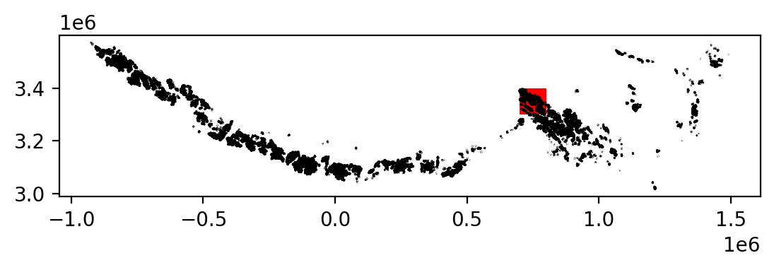
The plot above shows the coverage of the vector dataset, in black, relative to the extent of the raster dataset, in red. We will use the geopandas .clip() method to subset clip the RGI object (se_asia_prj) by the bbox_dc object which represents the footprint of the raster data cube.
#subset rgi to bounds
se_asia_subset = gpd.clip(se_asia_prj, bbox_dc)
se_asia_subset.head()
| rgi_id | o1region | o2region | glims_id | anlys_id | subm_id | src_date | cenlon | cenlat | utm_zone | ... | zmin_m | zmax_m | zmed_m | zmean_m | slope_deg | aspect_deg | aspect_sec | dem_source | lmax_m | geometry | |
|---|---|---|---|---|---|---|---|---|---|---|---|---|---|---|---|---|---|---|---|---|---|
| 16373 | RGI2000-v7.0-G-15-16374 | 15 | 15-03 | G095930E29817N | 930178 | 752 | 2005-09-08T00:00:00 | 95.929916 | 29.817003 | 46 | ... | 4985.7314 | 5274.0435 | 5142.7660 | 5148.8170 | 27.024134 | 139.048110 | 4 | COPDEM30 | 756 | POLYGON Z ((783110.719 3302487.481 0, 783148.4... |
| 16374 | RGI2000-v7.0-G-15-16375 | 15 | 15-03 | G095925E29818N | 930160 | 752 | 2005-09-08T00:00:00 | 95.925181 | 29.818399 | 46 | ... | 4856.2790 | 5054.9253 | 4929.5560 | 4933.6890 | 44.126980 | 211.518448 | 6 | COPDEM30 | 366 | POLYGON Z ((782511.36 3302381.154 0, 782534.76... |
| 16376 | RGI2000-v7.0-G-15-16377 | 15 | 15-03 | G095915E29820N | 930107 | 752 | 2005-09-08T00:00:00 | 95.914583 | 29.819510 | 46 | ... | 5072.8910 | 5150.6196 | 5108.5020 | 5111.7217 | 23.980000 | 219.341537 | 6 | COPDEM30 | 170 | POLYGON Z ((781619.822 3302305.074 0, 781613.5... |
| 16371 | RGI2000-v7.0-G-15-16372 | 15 | 15-03 | G095936E29819N | 930215 | 752 | 2005-09-08T00:00:00 | 95.935554 | 29.819123 | 46 | ... | 4838.7646 | 5194.8840 | 5001.5117 | 4992.3706 | 25.684517 | 128.737870 | 4 | COPDEM30 | 931 | POLYGON Z ((783420.055 3302493.804 0, 783444.1... |
| 15879 | RGI2000-v7.0-G-15-15880 | 15 | 15-03 | G095459E29807N | 928789 | 752 | 1999-07-29T00:00:00 | 95.459374 | 29.807181 | 46 | ... | 3802.1846 | 4155.1255 | 4000.2695 | 4000.4404 | 28.155806 | 116.148640 | 4 | COPDEM30 | 776 | POLYGON Z ((737667.211 3300277.169 0, 737702.8... |
5 rows × 29 columns
We can use the geopandas .explore() method to take a look at the RGI dataset:
se_asia_subset.explore()
/home/runner/micromamba/envs/itslive_tutorial_env/lib/python3.13/site-packages/folium/features.py:1173: UserWarning: GeoJsonTooltip is not configured to render for GeoJson GeometryCollection geometries. Please consider reworking these features: [{'rgi_id': 'RGI2000-v7.0-G-15-16433', 'o1region': '15', 'o2region': '15-03', 'glims_id': 'G095721E29941N', 'anlys_id': 929520, 'subm_id': 752, 'src_date': '2005-09-08T00:00:00', 'cenlon': 95.7211016152286, 'cenlat': 29.940902187781784, 'utm_zone': 46, 'area_km2': 0.340954350813452, 'primeclass': 0, 'conn_lvl': 0, 'surge_type': 0, 'term_type': 9, 'glac_name': None, 'is_rgi6': 0, 'termlon': 95.72222864596793, 'termlat': 29.937137080413784, 'zmin_m': 4657.792, 'zmax_m': 5049.5625, 'zmed_m': 4825.1104, 'zmean_m': 4839.4185, 'slope_deg': 23.704372, 'aspect_deg': 145.20973, 'aspect_sec': 4, 'dem_source': 'COPDEM30', 'lmax_m': 891}, {'rgi_id': 'RGI2000-v7.0-G-15-12194', 'o1region': '15', 'o2region': '15-03', 'glims_id': 'G095869E30315N', 'anlys_id': 929951, 'subm_id': 752, 'src_date': '2005-09-08T00:00:00', 'cenlon': 95.86889789565677, 'cenlat': 30.3147685, 'utm_zone': 46, 'area_km2': 8.797406997273084, 'primeclass': 0, 'conn_lvl': 0, 'surge_type': 0, 'term_type': 9, 'glac_name': None, 'is_rgi6': 0, 'termlon': 95.89518363763428, 'termlat': 30.307036248571297, 'zmin_m': 4642.1445, 'zmax_m': 5278.752, 'zmed_m': 5011.06, 'zmean_m': 4993.9243, 'slope_deg': 12.372513, 'aspect_deg': 81.418945, 'aspect_sec': 3, 'dem_source': 'COPDEM30', 'lmax_m': 4994}, {'rgi_id': 'RGI2000-v7.0-G-15-11941', 'o1region': '15', 'o2region': '15-03', 'glims_id': 'G095301E30377N', 'anlys_id': 928228, 'subm_id': 752, 'src_date': '2007-08-20T00:00:00', 'cenlon': 95.30071978915663, 'cenlat': 30.3770025, 'utm_zone': 46, 'area_km2': 0.267701958906151, 'primeclass': 0, 'conn_lvl': 0, 'surge_type': 0, 'term_type': 9, 'glac_name': None, 'is_rgi6': 0, 'termlon': 95.30345982475616, 'termlat': 30.380097687364806, 'zmin_m': 5475.784, 'zmax_m': 5977.979, 'zmed_m': 5750.727, 'zmean_m': 5759.621, 'slope_deg': 41.069595, 'aspect_deg': 350.3331518173218, 'aspect_sec': 1, 'dem_source': 'COPDEM30', 'lmax_m': 807}] to MultiPolygon for full functionality.
https://tools.ietf.org/html/rfc7946#page-9
warnings.warn(
Handling different geometry types#
Oops, it looks like we’re getting a warning on the explore() method. It looks like this is interfering with the functionality that displays feature info when you hover over a feature. Let’s dig into it and see what’s going on. It looks like the issue is being caused by rows of the GeoDataFrame object that have a ‘GeometryCollection’ geometry type. First, I’m going to copy the warning into a cell below. The warning is already in the form of a list of dictionaries, which makes it nice to work with:
Here is the error message separated from the problem geometries:
/home/../python3.11/site-packages/folium/features.py:1102: UserWarning: GeoJsonTooltip is not configured to render for GeoJson GeometryCollection geometries. Please consider reworking these features: ….. to MultiPolygon for full functionality.
And below are the problem geometries identified in the error message saved as a list of dictionaries:
problem_geoms = [{'rgi_id': 'RGI2000-v7.0-G-15-16433', 'o1region': '15', 'o2region': '15-03', 'glims_id': 'G095721E29941N', 'anlys_id': 929520, 'subm_id': 752, 'src_date': '2005-09-08T00:00:00', 'cenlon': 95.7211016152286, 'cenlat': 29.940902187781784, 'utm_zone': 46, 'area_km2': 0.340954350813452, 'primeclass': 0, 'conn_lvl': 0, 'surge_type': 0, 'term_type': 9, 'glac_name': None, 'is_rgi6': 0, 'termlon': 95.72222864596793, 'termlat': 29.937137080413784, 'zmin_m': 4657.792, 'zmax_m': 5049.5625, 'zmed_m': 4825.1104, 'zmean_m': 4839.4185, 'slope_deg': 23.704372, 'aspect_deg': 145.20973, 'aspect_sec': 4, 'dem_source': 'COPDEM30', 'lmax_m': 891},
{'rgi_id': 'RGI2000-v7.0-G-15-12194', 'o1region': '15', 'o2region': '15-03', 'glims_id': 'G095869E30315N', 'anlys_id': 929951, 'subm_id': 752, 'src_date': '2005-09-08T00:00:00', 'cenlon': 95.86889789565677, 'cenlat': 30.3147685, 'utm_zone': 46, 'area_km2': 8.797406997273084, 'primeclass': 0, 'conn_lvl': 0, 'surge_type': 0, 'term_type': 9, 'glac_name': None, 'is_rgi6': 0, 'termlon': 95.89518363763428, 'termlat': 30.307036248571297, 'zmin_m': 4642.1445, 'zmax_m': 5278.752, 'zmed_m': 5011.06, 'zmean_m': 4993.9243, 'slope_deg': 12.372513, 'aspect_deg': 81.418945, 'aspect_sec': 3, 'dem_source': 'COPDEM30', 'lmax_m': 4994},
{'rgi_id': 'RGI2000-v7.0-G-15-11941', 'o1region': '15', 'o2region': '15-03', 'glims_id': 'G095301E30377N', 'anlys_id': 928228, 'subm_id': 752, 'src_date': '2007-08-20T00:00:00', 'cenlon': 95.30071978915663, 'cenlat': 30.3770025, 'utm_zone': 46, 'area_km2': 0.267701958906151, 'primeclass': 0, 'conn_lvl': 0, 'surge_type': 0, 'term_type': 9, 'glac_name': None, 'is_rgi6': 0, 'termlon': 95.30345982475616, 'termlat': 30.380097687364806, 'zmin_m': 5475.784, 'zmax_m': 5977.979, 'zmed_m': 5750.727, 'zmean_m': 5759.621, 'slope_deg': 41.069595, 'aspect_deg': 350.3331518173218, 'aspect_sec': 1, 'dem_source': 'COPDEM30', 'lmax_m': 807}]
First, I’ll convert the problem_geoms object from a list of dictionary objects to a pandas.DataFrame object
problem_geoms_df = pd.DataFrame(data=problem_geoms)
Then make a list of the IDs of the glaciers in this dataframe:
problem_geom_ids = problem_geoms_df['glims_id'].to_list()
problem_geom_ids
['G095721E29941N', 'G095869E30315N', 'G095301E30377N']
We’ll make a geopandas.GeoDataFrame object that is just the above-identified outlines:
problem_geoms_gdf = se_asia_subset.loc[se_asia_subset['glims_id'].isin(problem_geom_ids)]
Now, let’s check the geometry-type of these outlines and compare them to another outline from the se_asia_subset object that wasn’t flagged:
problem_geoms_gdf.loc[problem_geoms_gdf['glims_id'] == 'G095301E30377N'].geom_type
11940 GeometryCollection
dtype: object
se_asia_subset.loc[se_asia_subset['rgi_id'] == 'RGI2000-v7.0-G-15-11754'].geom_type
11753 Polygon
dtype: object
Now the warning from calling geopandas.GeoDataFrame.explore() makes more sense. Most features in se_asia_subset have geom_type = Polygon but the flagged features have geom_type= GeometryCollection. Let’s dig a bit more into these flagged geometries. To do this, we can use the geopandas method explode() to split multiple geometries into multiple single geometries.
first_flagged_feature = problem_geoms_gdf[problem_geoms_gdf.glims_id == 'G095301E30377N'].geometry.explode(index_parts=True)
Printing this object shows that it actually contains a polygon geometry and a linestring geometry:
first_flagged_feature
11940 0 POLYGON Z ((721543.154 3362894.92 0, 721530.34...
1 LINESTRING Z (721119.337 3362535.315 0, 721119...
Name: geometry, dtype: geometry
Let’s look at the other two:
second_flagged_feature = problem_geoms_gdf[problem_geoms_gdf.glims_id == 'G095869E30315N'].geometry.explode(index_parts=True)
second_flagged_feature
12193 0 POLYGON Z ((774975.604 3356334.67 0, 774983.91...
1 LINESTRING Z (776713.643 3359150.691 0, 776713...
Name: geometry, dtype: geometry
third_flagged_feature = problem_geoms_gdf[problem_geoms_gdf.glims_id == 'G095721E29941N'].geometry.explode(index_parts=True)
third_flagged_feature
16432 0 POLYGON Z ((762550.755 3315675.227 0, 762550.8...
1 LINESTRING Z (762974.041 3315372.04 0, 762974....
Name: geometry, dtype: geometry
Let’s look at some properties of the line geometry objects like length:
print(third_flagged_feature[1:].length.iloc[0])
print(second_flagged_feature[1:].length.iloc[0])
print(third_flagged_feature[1:].length.iloc[0])
0.07253059141477144
0.07953751551272183
0.07253059141477144
It looks like all of the linestring objects are very small, possibly artifacts, and don’t need to remain in the dataset. For simplicity, we can remove them from the original object. There are different ways to do this, but here’s one approach:
Identify and remove all features with the
GeometryCollectiongeom_type:
se_asia_subset_polygon = se_asia_subset[~se_asia_subset['geometry'].apply(lambda x : x.geom_type=='GeometryCollection' )]
Remove the line geometries from the
GeometryCollectionfeatures:
se_asia_subset_geom_collection = se_asia_subset[se_asia_subset['geometry'].apply(lambda x : x.geom_type=='GeometryCollection' )]
Make an object that is just the features where
geom_type= Polygon:
keep_polygons = se_asia_subset_geom_collection.explode(index_parts=True).loc[se_asia_subset_geom_collection.explode(index_parts=True).geom_type == 'Polygon']
Append the polygons to the
se_asia_subset_polygonsobject:
se_asia_polygons = pd.concat([se_asia_subset_polygon,keep_polygons])
As a sanity check, let’s make sure that we didn’t lose any glacier outline features during all of that:
len(se_asia_subset['rgi_id']) == len(se_asia_polygons)
True
Great, we know that we have the same number of glaciers that we started with.
Now, let’s try visualizing the outlines with explore() again and seeing if the hover tools work:
se_asia_polygons.explore()
We can use the above interactive map to select a glacier to look at in more detail below.
Select a single glacier#
We’ll choose a single glacier to work with for now:
sample_glacier_vec = se_asia_subset.loc[se_asia_subset['rgi_id'] == 'RGI2000-v7.0-G-15-16257']
sample_glacier_vec
| rgi_id | o1region | o2region | glims_id | anlys_id | subm_id | src_date | cenlon | cenlat | utm_zone | ... | zmin_m | zmax_m | zmed_m | zmean_m | slope_deg | aspect_deg | aspect_sec | dem_source | lmax_m | geometry | |
|---|---|---|---|---|---|---|---|---|---|---|---|---|---|---|---|---|---|---|---|---|---|
| 16256 | RGI2000-v7.0-G-15-16257 | 15 | 15-03 | G095962E29920N | 930314 | 752 | 2005-09-08T00:00:00 | 95.961972 | 29.920094 | 46 | ... | 4320.7065 | 5937.84 | 5179.605 | 5131.8877 | 22.803406 | 100.811325 | 3 | COPDEM30 | 5958 | POLYGON Z ((788176.951 3315860.842 0, 788219.8... |
1 rows × 29 columns
Clip raster data using vector object#
Here we will subset the full ITS_LIVE granule to the extent of an individual glacier.
First, we need to use rio.write_crs() to assign a CRS to the itslive object. If we don’t do that first the rio.clip() command will produce an error
Note: you can only run write_crs() once, because it switches mapping from being a data_var to a coord so if you run it again it will produce a key error looking for a var that doesn’t exist
dc = dc.rio.write_crs(f"epsg:{dc.attrs['projection']}", inplace=True)
%%time
sample_glacier_raster = dc.rio.clip(sample_glacier_vec.geometry, sample_glacier_vec.crs)
CPU times: user 1.17 s, sys: 11 ms, total: 1.18 s
Wall time: 1.18 s
Working with clipped raster velocity data#
sample_glacier_raster
<xarray.Dataset> Size: 3GB
Dimensions: (mid_date: 47892, x: 40, y: 37)
Coordinates:
* mid_date (mid_date) datetime64[ns] 383kB 2022-06-07T04...
* x (x) float64 320B 7.843e+05 ... 7.889e+05
* y (y) float64 296B 3.316e+06 ... 3.311e+06
spatial_ref int64 8B 0
mapping int64 8B 0
Data variables: (12/59)
M11 (mid_date, y, x) float32 284MB dask.array<chunksize=(32736, 19, 19), meta=np.ndarray>
M11_dr_to_vr_factor (mid_date) float32 192kB dask.array<chunksize=(32736,), meta=np.ndarray>
M12 (mid_date, y, x) float32 284MB dask.array<chunksize=(32736, 19, 19), meta=np.ndarray>
M12_dr_to_vr_factor (mid_date) float32 192kB dask.array<chunksize=(32736,), meta=np.ndarray>
acquisition_date_img1 (mid_date) datetime64[ns] 383kB dask.array<chunksize=(32736,), meta=np.ndarray>
acquisition_date_img2 (mid_date) datetime64[ns] 383kB dask.array<chunksize=(32736,), meta=np.ndarray>
... ...
vy_error_modeled (mid_date) float32 192kB dask.array<chunksize=(32736,), meta=np.ndarray>
vy_error_slow (mid_date) float32 192kB dask.array<chunksize=(32736,), meta=np.ndarray>
vy_error_stationary (mid_date) float32 192kB dask.array<chunksize=(32736,), meta=np.ndarray>
vy_stable_shift (mid_date) float32 192kB dask.array<chunksize=(32736,), meta=np.ndarray>
vy_stable_shift_slow (mid_date) float32 192kB dask.array<chunksize=(32736,), meta=np.ndarray>
vy_stable_shift_stationary (mid_date) float32 192kB dask.array<chunksize=(32736,), meta=np.ndarray>
Attributes: (12/19)
Conventions: CF-1.8
GDAL_AREA_OR_POINT: Area
author: ITS_LIVE, a NASA MEaSUREs project (its-live.j...
autoRIFT_parameter_file: http://its-live-data.s3.amazonaws.com/autorif...
datacube_software_version: 1.0
date_created: 25-Sep-2023 22:00:23
... ...
s3: s3://its-live-data/datacubes/v2/N30E090/ITS_L...
skipped_granules: s3://its-live-data/datacubes/v2/N30E090/ITS_L...
time_standard_img1: UTC
time_standard_img2: UTC
title: ITS_LIVE datacube of image pair velocities
url: https://its-live-data.s3.amazonaws.com/datacu...- mid_date: 47892
- x: 40
- y: 37
- mid_date(mid_date)datetime64[ns]2022-06-07T04:21:44.211208960 .....
- description :
- midpoint of image 1 and image 2 acquisition date and time with granule's centroid longitude and latitude as microseconds
- standard_name :
- image_pair_center_date_with_time_separation
array(['2022-06-07T04:21:44.211208960', '2018-04-14T04:18:49.171219968', '2017-02-10T16:15:50.660901120', ..., '2024-01-23T04:18:19.231119104', '2023-06-01T04:10:44.893907968', '2023-09-02T16:18:20.230413056'], shape=(47892,), dtype='datetime64[ns]') - x(x)float647.843e+05 7.844e+05 ... 7.889e+05
- description :
- x coordinate of projection
- standard_name :
- projection_x_coordinate
- axis :
- X
- long_name :
- x coordinate of projection
- units :
- metre
array([784252.5, 784372.5, 784492.5, 784612.5, 784732.5, 784852.5, 784972.5, 785092.5, 785212.5, 785332.5, 785452.5, 785572.5, 785692.5, 785812.5, 785932.5, 786052.5, 786172.5, 786292.5, 786412.5, 786532.5, 786652.5, 786772.5, 786892.5, 787012.5, 787132.5, 787252.5, 787372.5, 787492.5, 787612.5, 787732.5, 787852.5, 787972.5, 788092.5, 788212.5, 788332.5, 788452.5, 788572.5, 788692.5, 788812.5, 788932.5]) - y(y)float643.316e+06 3.316e+06 ... 3.311e+06
- description :
- y coordinate of projection
- standard_name :
- projection_y_coordinate
- axis :
- Y
- long_name :
- y coordinate of projection
- units :
- metre
array([3315787.5, 3315667.5, 3315547.5, 3315427.5, 3315307.5, 3315187.5, 3315067.5, 3314947.5, 3314827.5, 3314707.5, 3314587.5, 3314467.5, 3314347.5, 3314227.5, 3314107.5, 3313987.5, 3313867.5, 3313747.5, 3313627.5, 3313507.5, 3313387.5, 3313267.5, 3313147.5, 3313027.5, 3312907.5, 3312787.5, 3312667.5, 3312547.5, 3312427.5, 3312307.5, 3312187.5, 3312067.5, 3311947.5, 3311827.5, 3311707.5, 3311587.5, 3311467.5]) - spatial_ref()int640
- GeoTransform :
- 784192.5 120.0 0.0 3315847.5 0.0 -120.0
array(0)
- mapping()int640
- crs_wkt :
- PROJCS["WGS 84 / UTM zone 46N",GEOGCS["WGS 84",DATUM["WGS_1984",SPHEROID["WGS 84",6378137,298.257223563,AUTHORITY["EPSG","7030"]],AUTHORITY["EPSG","6326"]],PRIMEM["Greenwich",0,AUTHORITY["EPSG","8901"]],UNIT["degree",0.0174532925199433,AUTHORITY["EPSG","9122"]],AUTHORITY["EPSG","4326"]],PROJECTION["Transverse_Mercator"],PARAMETER["latitude_of_origin",0],PARAMETER["central_meridian",93],PARAMETER["scale_factor",0.9996],PARAMETER["false_easting",500000],PARAMETER["false_northing",0],UNIT["metre",1,AUTHORITY["EPSG","9001"]],AXIS["Easting",EAST],AXIS["Northing",NORTH],AUTHORITY["EPSG","32646"]]
- semi_major_axis :
- 6378137.0
- semi_minor_axis :
- 6356752.314245179
- inverse_flattening :
- 298.257223563
- reference_ellipsoid_name :
- WGS 84
- longitude_of_prime_meridian :
- 0.0
- prime_meridian_name :
- Greenwich
- geographic_crs_name :
- WGS 84
- horizontal_datum_name :
- World Geodetic System 1984
- projected_crs_name :
- WGS 84 / UTM zone 46N
- grid_mapping_name :
- transverse_mercator
- latitude_of_projection_origin :
- 0.0
- longitude_of_central_meridian :
- 93.0
- false_easting :
- 500000.0
- false_northing :
- 0.0
- scale_factor_at_central_meridian :
- 0.9996
- spatial_ref :
- PROJCS["WGS 84 / UTM zone 46N",GEOGCS["WGS 84",DATUM["WGS_1984",SPHEROID["WGS 84",6378137,298.257223563,AUTHORITY["EPSG","7030"]],AUTHORITY["EPSG","6326"]],PRIMEM["Greenwich",0,AUTHORITY["EPSG","8901"]],UNIT["degree",0.0174532925199433,AUTHORITY["EPSG","9122"]],AUTHORITY["EPSG","4326"]],PROJECTION["Transverse_Mercator"],PARAMETER["latitude_of_origin",0],PARAMETER["central_meridian",93],PARAMETER["scale_factor",0.9996],PARAMETER["false_easting",500000],PARAMETER["false_northing",0],UNIT["metre",1,AUTHORITY["EPSG","9001"]],AXIS["Easting",EAST],AXIS["Northing",NORTH],AUTHORITY["EPSG","32646"]]
- GeoTransform :
- 784192.5 120.0 0.0 3315847.5 0.0 -120.0
array(0)
- M11(mid_date, y, x)float32dask.array<chunksize=(32736, 19, 19), meta=np.ndarray>
- description :
- conversion matrix element (1st row, 1st column) that can be multiplied with vx to give range pixel displacement dr (see Eq. A18 in https://www.mdpi.com/2072-4292/13/4/749)
- standard_name :
- conversion_matrix_element_11
- units :
- pixel/(meter/year)
Array Chunk Bytes 270.39 MiB 47.45 MiB Shape (47892, 37, 40) (32736, 19, 20) Dask graph 12 chunks in 7 graph layers Data type float32 numpy.ndarray - M11_dr_to_vr_factor(mid_date)float32dask.array<chunksize=(32736,), meta=np.ndarray>
- description :
- multiplicative factor that converts slant range pixel displacement dr to slant range velocity vr
- standard_name :
- M11_dr_to_vr_factor
- units :
- meter/(year*pixel)
Array Chunk Bytes 187.08 kiB 127.88 kiB Shape (47892,) (32736,) Dask graph 2 chunks in 3 graph layers Data type float32 numpy.ndarray - M12(mid_date, y, x)float32dask.array<chunksize=(32736, 19, 19), meta=np.ndarray>
- description :
- conversion matrix element (1st row, 2nd column) that can be multiplied with vy to give range pixel displacement dr (see Eq. A18 in https://www.mdpi.com/2072-4292/13/4/749)
- standard_name :
- conversion_matrix_element_12
- units :
- pixel/(meter/year)
Array Chunk Bytes 270.39 MiB 47.45 MiB Shape (47892, 37, 40) (32736, 19, 20) Dask graph 12 chunks in 7 graph layers Data type float32 numpy.ndarray - M12_dr_to_vr_factor(mid_date)float32dask.array<chunksize=(32736,), meta=np.ndarray>
- description :
- multiplicative factor that converts slant range pixel displacement dr to slant range velocity vr
- standard_name :
- M12_dr_to_vr_factor
- units :
- meter/(year*pixel)
Array Chunk Bytes 187.08 kiB 127.88 kiB Shape (47892,) (32736,) Dask graph 2 chunks in 3 graph layers Data type float32 numpy.ndarray - acquisition_date_img1(mid_date)datetime64[ns]dask.array<chunksize=(32736,), meta=np.ndarray>
- description :
- acquisition date and time of image 1
- standard_name :
- image1_acquition_date
Array Chunk Bytes 374.16 kiB 255.75 kiB Shape (47892,) (32736,) Dask graph 2 chunks in 3 graph layers Data type datetime64[ns] numpy.ndarray - acquisition_date_img2(mid_date)datetime64[ns]dask.array<chunksize=(32736,), meta=np.ndarray>
- description :
- acquisition date and time of image 2
- standard_name :
- image2_acquition_date
Array Chunk Bytes 374.16 kiB 255.75 kiB Shape (47892,) (32736,) Dask graph 2 chunks in 3 graph layers Data type datetime64[ns] numpy.ndarray - autoRIFT_software_version(mid_date)<U5dask.array<chunksize=(32736,), meta=np.ndarray>
- description :
- version of autoRIFT software
- standard_name :
- autoRIFT_software_version
Array Chunk Bytes 0.91 MiB 639.38 kiB Shape (47892,) (32736,) Dask graph 2 chunks in 3 graph layers Data type - chip_size_height(mid_date, y, x)float32dask.array<chunksize=(32736, 19, 19), meta=np.ndarray>
- chip_size_coordinates :
- Optical data: chip_size_coordinates = 'image projection geometry: width = x, height = y'. Radar data: chip_size_coordinates = 'radar geometry: width = range, height = azimuth'
- description :
- height of search template (chip)
- standard_name :
- chip_size_height
- units :
- m
- y_pixel_size :
- 10.0
Array Chunk Bytes 270.39 MiB 47.45 MiB Shape (47892, 37, 40) (32736, 19, 20) Dask graph 12 chunks in 7 graph layers Data type float32 numpy.ndarray - chip_size_width(mid_date, y, x)float32dask.array<chunksize=(32736, 19, 19), meta=np.ndarray>
- chip_size_coordinates :
- Optical data: chip_size_coordinates = 'image projection geometry: width = x, height = y'. Radar data: chip_size_coordinates = 'radar geometry: width = range, height = azimuth'
- description :
- width of search template (chip)
- standard_name :
- chip_size_width
- units :
- m
- x_pixel_size :
- 10.0
Array Chunk Bytes 270.39 MiB 47.45 MiB Shape (47892, 37, 40) (32736, 19, 20) Dask graph 12 chunks in 7 graph layers Data type float32 numpy.ndarray - date_center(mid_date)datetime64[ns]dask.array<chunksize=(32736,), meta=np.ndarray>
- description :
- midpoint of image 1 and image 2 acquisition date
- standard_name :
- image_pair_center_date
Array Chunk Bytes 374.16 kiB 255.75 kiB Shape (47892,) (32736,) Dask graph 2 chunks in 3 graph layers Data type datetime64[ns] numpy.ndarray - date_dt(mid_date)timedelta64[ns]dask.array<chunksize=(32736,), meta=np.ndarray>
- description :
- time separation between acquisition of image 1 and image 2
- standard_name :
- image_pair_time_separation
Array Chunk Bytes 374.16 kiB 255.75 kiB Shape (47892,) (32736,) Dask graph 2 chunks in 3 graph layers Data type timedelta64[ns] numpy.ndarray - floatingice(y, x)float32dask.array<chunksize=(19, 19), meta=np.ndarray>
- description :
- floating ice mask, 0 = non-floating-ice, 1 = floating-ice
- flag_meanings :
- non-ice ice
- flag_values :
- [0, 1]
- standard_name :
- floating ice mask
- url :
- https://its-live-data.s3.amazonaws.com/autorift_parameters/v001/N46_0120m_floatingice.tif
Array Chunk Bytes 5.78 kiB 1.48 kiB Shape (37, 40) (19, 20) Dask graph 6 chunks in 7 graph layers Data type float32 numpy.ndarray - granule_url(mid_date)<U1024dask.array<chunksize=(32736,), meta=np.ndarray>
- description :
- original granule URL
- standard_name :
- granule_url
Array Chunk Bytes 187.08 MiB 127.88 MiB Shape (47892,) (32736,) Dask graph 2 chunks in 2 graph layers Data type - interp_mask(mid_date, y, x)float32dask.array<chunksize=(32736, 19, 19), meta=np.ndarray>
- description :
- light interpolation mask
- flag_meanings :
- measured interpolated
- flag_values :
- [0, 1]
- standard_name :
- interpolated_value_mask
Array Chunk Bytes 270.39 MiB 47.45 MiB Shape (47892, 37, 40) (32736, 19, 20) Dask graph 12 chunks in 7 graph layers Data type float32 numpy.ndarray - landice(y, x)float32dask.array<chunksize=(19, 19), meta=np.ndarray>
- description :
- land ice mask, 0 = non-land-ice, 1 = land-ice
- flag_meanings :
- non-ice ice
- flag_values :
- [0, 1]
- standard_name :
- land ice mask
- url :
- https://its-live-data.s3.amazonaws.com/autorift_parameters/v001/N46_0120m_landice.tif
Array Chunk Bytes 5.78 kiB 1.48 kiB Shape (37, 40) (19, 20) Dask graph 6 chunks in 7 graph layers Data type float32 numpy.ndarray - mission_img1(mid_date)<U1dask.array<chunksize=(32736,), meta=np.ndarray>
- description :
- id of the mission that acquired image 1
- standard_name :
- image1_mission
Array Chunk Bytes 187.08 kiB 127.88 kiB Shape (47892,) (32736,) Dask graph 2 chunks in 3 graph layers Data type - mission_img2(mid_date)<U1dask.array<chunksize=(32736,), meta=np.ndarray>
- description :
- id of the mission that acquired image 2
- standard_name :
- image2_mission
Array Chunk Bytes 187.08 kiB 127.88 kiB Shape (47892,) (32736,) Dask graph 2 chunks in 3 graph layers Data type - roi_valid_percentage(mid_date)float32dask.array<chunksize=(32736,), meta=np.ndarray>
- description :
- percentage of pixels with a valid velocity estimate determined for the intersection of the full image pair footprint and the region of interest (roi) that defines where autoRIFT tried to estimate a velocity
- standard_name :
- region_of_interest_valid_pixel_percentage
Array Chunk Bytes 187.08 kiB 127.88 kiB Shape (47892,) (32736,) Dask graph 2 chunks in 3 graph layers Data type float32 numpy.ndarray - satellite_img1(mid_date)<U2dask.array<chunksize=(32736,), meta=np.ndarray>
- description :
- id of the satellite that acquired image 1
- standard_name :
- image1_satellite
Array Chunk Bytes 374.16 kiB 255.75 kiB Shape (47892,) (32736,) Dask graph 2 chunks in 3 graph layers Data type - satellite_img2(mid_date)<U2dask.array<chunksize=(32736,), meta=np.ndarray>
- description :
- id of the satellite that acquired image 2
- standard_name :
- image2_satellite
Array Chunk Bytes 374.16 kiB 255.75 kiB Shape (47892,) (32736,) Dask graph 2 chunks in 3 graph layers Data type - sensor_img1(mid_date)<U3dask.array<chunksize=(32736,), meta=np.ndarray>
- description :
- id of the sensor that acquired image 1
- standard_name :
- image1_sensor
Array Chunk Bytes 561.23 kiB 383.62 kiB Shape (47892,) (32736,) Dask graph 2 chunks in 3 graph layers Data type - sensor_img2(mid_date)<U3dask.array<chunksize=(32736,), meta=np.ndarray>
- description :
- id of the sensor that acquired image 2
- standard_name :
- image2_sensor
Array Chunk Bytes 561.23 kiB 383.62 kiB Shape (47892,) (32736,) Dask graph 2 chunks in 3 graph layers Data type - stable_count_slow(mid_date)uint16dask.array<chunksize=(32736,), meta=np.ndarray>
- description :
- number of valid pixels over slowest 25% of ice
- standard_name :
- stable_count_slow
- units :
- count
Array Chunk Bytes 93.54 kiB 63.94 kiB Shape (47892,) (32736,) Dask graph 2 chunks in 3 graph layers Data type uint16 numpy.ndarray - stable_count_stationary(mid_date)uint16dask.array<chunksize=(32736,), meta=np.ndarray>
- description :
- number of valid pixels over stationary or slow-flowing surfaces
- standard_name :
- stable_count_stationary
- units :
- count
Array Chunk Bytes 93.54 kiB 63.94 kiB Shape (47892,) (32736,) Dask graph 2 chunks in 3 graph layers Data type uint16 numpy.ndarray - stable_shift_flag(mid_date)uint8dask.array<chunksize=(32736,), meta=np.ndarray>
- description :
- flag for applying velocity bias correction: 0 = no correction; 1 = correction from overlapping stable surface mask (stationary or slow-flowing surfaces with velocity < 15 m/yr)(top priority); 2 = correction from slowest 25% of overlapping velocities (second priority)
- standard_name :
- stable_shift_flag
Array Chunk Bytes 46.77 kiB 31.97 kiB Shape (47892,) (32736,) Dask graph 2 chunks in 3 graph layers Data type uint8 numpy.ndarray - v(mid_date, y, x)float32dask.array<chunksize=(32736, 19, 19), meta=np.ndarray>
- description :
- velocity magnitude
- standard_name :
- land_ice_surface_velocity
- units :
- meter/year
Array Chunk Bytes 270.39 MiB 47.45 MiB Shape (47892, 37, 40) (32736, 19, 20) Dask graph 12 chunks in 7 graph layers Data type float32 numpy.ndarray - v_error(mid_date, y, x)float32dask.array<chunksize=(32736, 19, 19), meta=np.ndarray>
- description :
- velocity magnitude error
- standard_name :
- velocity_error
- units :
- meter/year
Array Chunk Bytes 270.39 MiB 47.45 MiB Shape (47892, 37, 40) (32736, 19, 20) Dask graph 12 chunks in 7 graph layers Data type float32 numpy.ndarray - va(mid_date, y, x)float32dask.array<chunksize=(32736, 19, 19), meta=np.ndarray>
- description :
- velocity in radar azimuth direction
Array Chunk Bytes 270.39 MiB 47.45 MiB Shape (47892, 37, 40) (32736, 19, 20) Dask graph 12 chunks in 7 graph layers Data type float32 numpy.ndarray - va_error(mid_date)float32dask.array<chunksize=(32736,), meta=np.ndarray>
- description :
- error for velocity in radar azimuth direction
- standard_name :
- va_error
- units :
- meter/year
Array Chunk Bytes 187.08 kiB 127.88 kiB Shape (47892,) (32736,) Dask graph 2 chunks in 3 graph layers Data type float32 numpy.ndarray - va_error_modeled(mid_date)float32dask.array<chunksize=(32736,), meta=np.ndarray>
- description :
- 1-sigma error calculated using a modeled error-dt relationship
- standard_name :
- va_error_modeled
- units :
- meter/year
Array Chunk Bytes 187.08 kiB 127.88 kiB Shape (47892,) (32736,) Dask graph 2 chunks in 3 graph layers Data type float32 numpy.ndarray - va_error_slow(mid_date)float32dask.array<chunksize=(32736,), meta=np.ndarray>
- description :
- RMSE over slowest 25% of retrieved velocities
- standard_name :
- va_error_slow
- units :
- meter/year
Array Chunk Bytes 187.08 kiB 127.88 kiB Shape (47892,) (32736,) Dask graph 2 chunks in 3 graph layers Data type float32 numpy.ndarray - va_error_stationary(mid_date)float32dask.array<chunksize=(32736,), meta=np.ndarray>
- description :
- RMSE over stable surfaces, stationary or slow-flowing surfaces with velocity < 15 m/yr identified from an external mask
- standard_name :
- va_error_stationary
- units :
- meter/year
Array Chunk Bytes 187.08 kiB 127.88 kiB Shape (47892,) (32736,) Dask graph 2 chunks in 3 graph layers Data type float32 numpy.ndarray - va_stable_shift(mid_date)float32dask.array<chunksize=(32736,), meta=np.ndarray>
- description :
- applied va shift calibrated using pixels over stable or slow surfaces
- standard_name :
- va_stable_shift
- units :
- meter/year
Array Chunk Bytes 187.08 kiB 127.88 kiB Shape (47892,) (32736,) Dask graph 2 chunks in 3 graph layers Data type float32 numpy.ndarray - va_stable_shift_slow(mid_date)float32dask.array<chunksize=(32736,), meta=np.ndarray>
- description :
- va shift calibrated using valid pixels over slowest 25% of retrieved velocities
- standard_name :
- va_stable_shift_slow
- units :
- meter/year
Array Chunk Bytes 187.08 kiB 127.88 kiB Shape (47892,) (32736,) Dask graph 2 chunks in 3 graph layers Data type float32 numpy.ndarray - va_stable_shift_stationary(mid_date)float32dask.array<chunksize=(32736,), meta=np.ndarray>
- description :
- va shift calibrated using valid pixels over stable surfaces, stationary or slow-flowing surfaces with velocity < 15 m/yr identified from an external mask
- standard_name :
- va_stable_shift_stationary
- units :
- meter/year
Array Chunk Bytes 187.08 kiB 127.88 kiB Shape (47892,) (32736,) Dask graph 2 chunks in 3 graph layers Data type float32 numpy.ndarray - vr(mid_date, y, x)float32dask.array<chunksize=(32736, 19, 19), meta=np.ndarray>
- description :
- velocity in radar range direction
Array Chunk Bytes 270.39 MiB 47.45 MiB Shape (47892, 37, 40) (32736, 19, 20) Dask graph 12 chunks in 7 graph layers Data type float32 numpy.ndarray - vr_error(mid_date)float32dask.array<chunksize=(32736,), meta=np.ndarray>
- description :
- error for velocity in radar range direction
- standard_name :
- vr_error
- units :
- meter/year
Array Chunk Bytes 187.08 kiB 127.88 kiB Shape (47892,) (32736,) Dask graph 2 chunks in 3 graph layers Data type float32 numpy.ndarray - vr_error_modeled(mid_date)float32dask.array<chunksize=(32736,), meta=np.ndarray>
- description :
- 1-sigma error calculated using a modeled error-dt relationship
- standard_name :
- vr_error_modeled
- units :
- meter/year
Array Chunk Bytes 187.08 kiB 127.88 kiB Shape (47892,) (32736,) Dask graph 2 chunks in 3 graph layers Data type float32 numpy.ndarray - vr_error_slow(mid_date)float32dask.array<chunksize=(32736,), meta=np.ndarray>
- description :
- RMSE over slowest 25% of retrieved velocities
- standard_name :
- vr_error_slow
- units :
- meter/year
Array Chunk Bytes 187.08 kiB 127.88 kiB Shape (47892,) (32736,) Dask graph 2 chunks in 3 graph layers Data type float32 numpy.ndarray - vr_error_stationary(mid_date)float32dask.array<chunksize=(32736,), meta=np.ndarray>
- description :
- RMSE over stable surfaces, stationary or slow-flowing surfaces with velocity < 15 m/yr identified from an external mask
- standard_name :
- vr_error_stationary
- units :
- meter/year
Array Chunk Bytes 187.08 kiB 127.88 kiB Shape (47892,) (32736,) Dask graph 2 chunks in 3 graph layers Data type float32 numpy.ndarray - vr_stable_shift(mid_date)float32dask.array<chunksize=(32736,), meta=np.ndarray>
- description :
- applied vr shift calibrated using pixels over stable or slow surfaces
- standard_name :
- vr_stable_shift
- units :
- meter/year
Array Chunk Bytes 187.08 kiB 127.88 kiB Shape (47892,) (32736,) Dask graph 2 chunks in 3 graph layers Data type float32 numpy.ndarray - vr_stable_shift_slow(mid_date)float32dask.array<chunksize=(32736,), meta=np.ndarray>
- description :
- vr shift calibrated using valid pixels over slowest 25% of retrieved velocities
- standard_name :
- vr_stable_shift_slow
- units :
- meter/year
Array Chunk Bytes 187.08 kiB 127.88 kiB Shape (47892,) (32736,) Dask graph 2 chunks in 3 graph layers Data type float32 numpy.ndarray - vr_stable_shift_stationary(mid_date)float32dask.array<chunksize=(32736,), meta=np.ndarray>
- description :
- vr shift calibrated using valid pixels over stable surfaces, stationary or slow-flowing surfaces with velocity < 15 m/yr identified from an external mask
- standard_name :
- vr_stable_shift_stationary
- units :
- meter/year
Array Chunk Bytes 187.08 kiB 127.88 kiB Shape (47892,) (32736,) Dask graph 2 chunks in 3 graph layers Data type float32 numpy.ndarray - vx(mid_date, y, x)float32dask.array<chunksize=(32736, 19, 19), meta=np.ndarray>
- description :
- velocity component in x direction
- standard_name :
- land_ice_surface_x_velocity
- units :
- meter/year
Array Chunk Bytes 270.39 MiB 47.45 MiB Shape (47892, 37, 40) (32736, 19, 20) Dask graph 12 chunks in 7 graph layers Data type float32 numpy.ndarray - vx_error(mid_date)float32dask.array<chunksize=(32736,), meta=np.ndarray>
- description :
- best estimate of x_velocity error: vx_error is populated according to the approach used for the velocity bias correction as indicated in "stable_shift_flag"
- standard_name :
- vx_error
- units :
- meter/year
Array Chunk Bytes 187.08 kiB 127.88 kiB Shape (47892,) (32736,) Dask graph 2 chunks in 3 graph layers Data type float32 numpy.ndarray - vx_error_modeled(mid_date)float32dask.array<chunksize=(32736,), meta=np.ndarray>
- description :
- 1-sigma error calculated using a modeled error-dt relationship
- standard_name :
- vx_error_modeled
- units :
- meter/year
Array Chunk Bytes 187.08 kiB 127.88 kiB Shape (47892,) (32736,) Dask graph 2 chunks in 3 graph layers Data type float32 numpy.ndarray - vx_error_slow(mid_date)float32dask.array<chunksize=(32736,), meta=np.ndarray>
- description :
- RMSE over slowest 25% of retrieved velocities
- standard_name :
- vx_error_slow
- units :
- meter/year
Array Chunk Bytes 187.08 kiB 127.88 kiB Shape (47892,) (32736,) Dask graph 2 chunks in 3 graph layers Data type float32 numpy.ndarray - vx_error_stationary(mid_date)float32dask.array<chunksize=(32736,), meta=np.ndarray>
- description :
- RMSE over stable surfaces, stationary or slow-flowing surfaces with velocity < 15 meter/year identified from an external mask
- standard_name :
- vx_error_stationary
- units :
- meter/year
Array Chunk Bytes 187.08 kiB 127.88 kiB Shape (47892,) (32736,) Dask graph 2 chunks in 3 graph layers Data type float32 numpy.ndarray - vx_stable_shift(mid_date)float32dask.array<chunksize=(32736,), meta=np.ndarray>
- description :
- applied vx shift calibrated using pixels over stable or slow surfaces
- standard_name :
- vx_stable_shift
- units :
- meter/year
Array Chunk Bytes 187.08 kiB 127.88 kiB Shape (47892,) (32736,) Dask graph 2 chunks in 3 graph layers Data type float32 numpy.ndarray - vx_stable_shift_slow(mid_date)float32dask.array<chunksize=(32736,), meta=np.ndarray>
- description :
- vx shift calibrated using valid pixels over slowest 25% of retrieved velocities
- standard_name :
- vx_stable_shift_slow
- units :
- meter/year
Array Chunk Bytes 187.08 kiB 127.88 kiB Shape (47892,) (32736,) Dask graph 2 chunks in 3 graph layers Data type float32 numpy.ndarray - vx_stable_shift_stationary(mid_date)float32dask.array<chunksize=(32736,), meta=np.ndarray>
- description :
- vx shift calibrated using valid pixels over stable surfaces, stationary or slow-flowing surfaces with velocity < 15 m/yr identified from an external mask
- standard_name :
- vx_stable_shift_stationary
- units :
- meter/year
Array Chunk Bytes 187.08 kiB 127.88 kiB Shape (47892,) (32736,) Dask graph 2 chunks in 3 graph layers Data type float32 numpy.ndarray - vy(mid_date, y, x)float32dask.array<chunksize=(32736, 19, 19), meta=np.ndarray>
- description :
- velocity component in y direction
- standard_name :
- land_ice_surface_y_velocity
- units :
- meter/year
Array Chunk Bytes 270.39 MiB 47.45 MiB Shape (47892, 37, 40) (32736, 19, 20) Dask graph 12 chunks in 7 graph layers Data type float32 numpy.ndarray - vy_error(mid_date)float32dask.array<chunksize=(32736,), meta=np.ndarray>
- description :
- best estimate of y_velocity error: vy_error is populated according to the approach used for the velocity bias correction as indicated in "stable_shift_flag"
- standard_name :
- vy_error
- units :
- meter/year
Array Chunk Bytes 187.08 kiB 127.88 kiB Shape (47892,) (32736,) Dask graph 2 chunks in 3 graph layers Data type float32 numpy.ndarray - vy_error_modeled(mid_date)float32dask.array<chunksize=(32736,), meta=np.ndarray>
- description :
- 1-sigma error calculated using a modeled error-dt relationship
- standard_name :
- vy_error_modeled
- units :
- meter/year
Array Chunk Bytes 187.08 kiB 127.88 kiB Shape (47892,) (32736,) Dask graph 2 chunks in 3 graph layers Data type float32 numpy.ndarray - vy_error_slow(mid_date)float32dask.array<chunksize=(32736,), meta=np.ndarray>
- description :
- RMSE over slowest 25% of retrieved velocities
- standard_name :
- vy_error_slow
- units :
- meter/year
Array Chunk Bytes 187.08 kiB 127.88 kiB Shape (47892,) (32736,) Dask graph 2 chunks in 3 graph layers Data type float32 numpy.ndarray - vy_error_stationary(mid_date)float32dask.array<chunksize=(32736,), meta=np.ndarray>
- description :
- RMSE over stable surfaces, stationary or slow-flowing surfaces with velocity < 15 meter/year identified from an external mask
- standard_name :
- vy_error_stationary
- units :
- meter/year
Array Chunk Bytes 187.08 kiB 127.88 kiB Shape (47892,) (32736,) Dask graph 2 chunks in 3 graph layers Data type float32 numpy.ndarray - vy_stable_shift(mid_date)float32dask.array<chunksize=(32736,), meta=np.ndarray>
- description :
- applied vy shift calibrated using pixels over stable or slow surfaces
- standard_name :
- vy_stable_shift
- units :
- meter/year
Array Chunk Bytes 187.08 kiB 127.88 kiB Shape (47892,) (32736,) Dask graph 2 chunks in 3 graph layers Data type float32 numpy.ndarray - vy_stable_shift_slow(mid_date)float32dask.array<chunksize=(32736,), meta=np.ndarray>
- description :
- vy shift calibrated using valid pixels over slowest 25% of retrieved velocities
- standard_name :
- vy_stable_shift_slow
- units :
- meter/year
Array Chunk Bytes 187.08 kiB 127.88 kiB Shape (47892,) (32736,) Dask graph 2 chunks in 3 graph layers Data type float32 numpy.ndarray - vy_stable_shift_stationary(mid_date)float32dask.array<chunksize=(32736,), meta=np.ndarray>
- description :
- vy shift calibrated using valid pixels over stable surfaces, stationary or slow-flowing surfaces with velocity < 15 m/yr identified from an external mask
- standard_name :
- vy_stable_shift_stationary
- units :
- meter/year
Array Chunk Bytes 187.08 kiB 127.88 kiB Shape (47892,) (32736,) Dask graph 2 chunks in 3 graph layers Data type float32 numpy.ndarray
- mid_datePandasIndex
PandasIndex(DatetimeIndex(['2022-06-07 04:21:44.211208960', '2018-04-14 04:18:49.171219968', '2017-02-10 16:15:50.660901120', '2022-04-03 04:19:01.211214080', '2021-07-22 04:16:46.210427904', '2019-03-15 04:15:44.180925952', '2002-09-15 03:59:12.379172096', '2002-12-28 03:42:16.181281024', '2021-06-29 16:16:10.210323968', '2022-03-26 16:18:35.211123968', ... '2021-10-05 04:15:51.210407936', '2022-11-11 16:15:55.220602112', '2022-06-29 16:19:50.211113984', '2023-08-18 16:18:10.230522880', '2023-08-03 16:18:00.221108992', '2022-12-16 16:16:00.220919808', '2023-02-12 04:15:56.220721920', '2024-01-23 04:18:19.231119104', '2023-06-01 04:10:44.893907968', '2023-09-02 16:18:20.230413056'], dtype='datetime64[ns]', name='mid_date', length=47892, freq=None)) - xPandasIndex
PandasIndex(Index([784252.5, 784372.5, 784492.5, 784612.5, 784732.5, 784852.5, 784972.5, 785092.5, 785212.5, 785332.5, 785452.5, 785572.5, 785692.5, 785812.5, 785932.5, 786052.5, 786172.5, 786292.5, 786412.5, 786532.5, 786652.5, 786772.5, 786892.5, 787012.5, 787132.5, 787252.5, 787372.5, 787492.5, 787612.5, 787732.5, 787852.5, 787972.5, 788092.5, 788212.5, 788332.5, 788452.5, 788572.5, 788692.5, 788812.5, 788932.5], dtype='float64', name='x')) - yPandasIndex
PandasIndex(Index([3315787.5, 3315667.5, 3315547.5, 3315427.5, 3315307.5, 3315187.5, 3315067.5, 3314947.5, 3314827.5, 3314707.5, 3314587.5, 3314467.5, 3314347.5, 3314227.5, 3314107.5, 3313987.5, 3313867.5, 3313747.5, 3313627.5, 3313507.5, 3313387.5, 3313267.5, 3313147.5, 3313027.5, 3312907.5, 3312787.5, 3312667.5, 3312547.5, 3312427.5, 3312307.5, 3312187.5, 3312067.5, 3311947.5, 3311827.5, 3311707.5, 3311587.5, 3311467.5], dtype='float64', name='y'))
- Conventions :
- CF-1.8
- GDAL_AREA_OR_POINT :
- Area
- author :
- ITS_LIVE, a NASA MEaSUREs project (its-live.jpl.nasa.gov)
- autoRIFT_parameter_file :
- http://its-live-data.s3.amazonaws.com/autorift_parameters/v001/autorift_landice_0120m.shp
- datacube_software_version :
- 1.0
- date_created :
- 25-Sep-2023 22:00:23
- date_updated :
- 13-Nov-2024 00:08:07
- geo_polygon :
- [[95.06959008486952, 29.814255053135895], [95.32812062059084, 29.809951334550703], [95.58659184122865, 29.80514261876954], [95.84499718862224, 29.7998293459177], [96.10333011481168, 29.79401200205343], [96.11032804508507, 30.019297601073085], [96.11740568350054, 30.244573983323825], [96.12456379063154, 30.469841094022847], [96.1318031397002, 30.695098878594504], [95.87110827645229, 30.70112924501256], [95.61033817656023, 30.7066371044805], [95.34949964126946, 30.711621947056347], [95.08859948278467, 30.716083310981194], [95.08376623410525, 30.49063893600811], [95.07898726183609, 30.26518607254204], [95.0742620484426, 30.039724763743482], [95.06959008486952, 29.814255053135895]]
- institution :
- NASA Jet Propulsion Laboratory (JPL), California Institute of Technology
- latitude :
- 30.26
- longitude :
- 95.6
- proj_polygon :
- [[700000, 3300000], [725000.0, 3300000.0], [750000.0, 3300000.0], [775000.0, 3300000.0], [800000, 3300000], [800000.0, 3325000.0], [800000.0, 3350000.0], [800000.0, 3375000.0], [800000, 3400000], [775000.0, 3400000.0], [750000.0, 3400000.0], [725000.0, 3400000.0], [700000, 3400000], [700000.0, 3375000.0], [700000.0, 3350000.0], [700000.0, 3325000.0], [700000, 3300000]]
- projection :
- 32646
- s3 :
- s3://its-live-data/datacubes/v2/N30E090/ITS_LIVE_vel_EPSG32646_G0120_X750000_Y3350000.zarr
- skipped_granules :
- s3://its-live-data/datacubes/v2/N30E090/ITS_LIVE_vel_EPSG32646_G0120_X750000_Y3350000.json
- time_standard_img1 :
- UTC
- time_standard_img2 :
- UTC
- title :
- ITS_LIVE datacube of image pair velocities
- url :
- https://its-live-data.s3.amazonaws.com/datacubes/v2/N30E090/ITS_LIVE_vel_EPSG32646_G0120_X750000_Y3350000.zarr
Take a look at the clipped object:
sample_glacier_raster.mid_date
<xarray.DataArray 'mid_date' (mid_date: 47892)> Size: 383kB
array(['2022-06-07T04:21:44.211208960', '2018-04-14T04:18:49.171219968',
'2017-02-10T16:15:50.660901120', ..., '2024-01-23T04:18:19.231119104',
'2023-06-01T04:10:44.893907968', '2023-09-02T16:18:20.230413056'],
shape=(47892,), dtype='datetime64[ns]')
Coordinates:
* mid_date (mid_date) datetime64[ns] 383kB 2022-06-07T04:21:44.21120896...
spatial_ref int64 8B 0
mapping int64 8B 0
Attributes:
description: midpoint of image 1 and image 2 acquisition date and time...
standard_name: image_pair_center_date_with_time_separation- mid_date: 47892
- 2022-06-07T04:21:44.211208960 ... 2023-09-02T16:18:20.230413056
array(['2022-06-07T04:21:44.211208960', '2018-04-14T04:18:49.171219968', '2017-02-10T16:15:50.660901120', ..., '2024-01-23T04:18:19.231119104', '2023-06-01T04:10:44.893907968', '2023-09-02T16:18:20.230413056'], shape=(47892,), dtype='datetime64[ns]') - mid_date(mid_date)datetime64[ns]2022-06-07T04:21:44.211208960 .....
- description :
- midpoint of image 1 and image 2 acquisition date and time with granule's centroid longitude and latitude as microseconds
- standard_name :
- image_pair_center_date_with_time_separation
array(['2022-06-07T04:21:44.211208960', '2018-04-14T04:18:49.171219968', '2017-02-10T16:15:50.660901120', ..., '2024-01-23T04:18:19.231119104', '2023-06-01T04:10:44.893907968', '2023-09-02T16:18:20.230413056'], shape=(47892,), dtype='datetime64[ns]') - spatial_ref()int640
- GeoTransform :
- 784192.5 120.0 0.0 3315847.5 0.0 -120.0
array(0)
- mapping()int640
- crs_wkt :
- PROJCS["WGS 84 / UTM zone 46N",GEOGCS["WGS 84",DATUM["WGS_1984",SPHEROID["WGS 84",6378137,298.257223563,AUTHORITY["EPSG","7030"]],AUTHORITY["EPSG","6326"]],PRIMEM["Greenwich",0,AUTHORITY["EPSG","8901"]],UNIT["degree",0.0174532925199433,AUTHORITY["EPSG","9122"]],AUTHORITY["EPSG","4326"]],PROJECTION["Transverse_Mercator"],PARAMETER["latitude_of_origin",0],PARAMETER["central_meridian",93],PARAMETER["scale_factor",0.9996],PARAMETER["false_easting",500000],PARAMETER["false_northing",0],UNIT["metre",1,AUTHORITY["EPSG","9001"]],AXIS["Easting",EAST],AXIS["Northing",NORTH],AUTHORITY["EPSG","32646"]]
- semi_major_axis :
- 6378137.0
- semi_minor_axis :
- 6356752.314245179
- inverse_flattening :
- 298.257223563
- reference_ellipsoid_name :
- WGS 84
- longitude_of_prime_meridian :
- 0.0
- prime_meridian_name :
- Greenwich
- geographic_crs_name :
- WGS 84
- horizontal_datum_name :
- World Geodetic System 1984
- projected_crs_name :
- WGS 84 / UTM zone 46N
- grid_mapping_name :
- transverse_mercator
- latitude_of_projection_origin :
- 0.0
- longitude_of_central_meridian :
- 93.0
- false_easting :
- 500000.0
- false_northing :
- 0.0
- scale_factor_at_central_meridian :
- 0.9996
- spatial_ref :
- PROJCS["WGS 84 / UTM zone 46N",GEOGCS["WGS 84",DATUM["WGS_1984",SPHEROID["WGS 84",6378137,298.257223563,AUTHORITY["EPSG","7030"]],AUTHORITY["EPSG","6326"]],PRIMEM["Greenwich",0,AUTHORITY["EPSG","8901"]],UNIT["degree",0.0174532925199433,AUTHORITY["EPSG","9122"]],AUTHORITY["EPSG","4326"]],PROJECTION["Transverse_Mercator"],PARAMETER["latitude_of_origin",0],PARAMETER["central_meridian",93],PARAMETER["scale_factor",0.9996],PARAMETER["false_easting",500000],PARAMETER["false_northing",0],UNIT["metre",1,AUTHORITY["EPSG","9001"]],AXIS["Easting",EAST],AXIS["Northing",NORTH],AUTHORITY["EPSG","32646"]]
- GeoTransform :
- 784192.5 120.0 0.0 3315847.5 0.0 -120.0
array(0)
- mid_datePandasIndex
PandasIndex(DatetimeIndex(['2022-06-07 04:21:44.211208960', '2018-04-14 04:18:49.171219968', '2017-02-10 16:15:50.660901120', '2022-04-03 04:19:01.211214080', '2021-07-22 04:16:46.210427904', '2019-03-15 04:15:44.180925952', '2002-09-15 03:59:12.379172096', '2002-12-28 03:42:16.181281024', '2021-06-29 16:16:10.210323968', '2022-03-26 16:18:35.211123968', ... '2021-10-05 04:15:51.210407936', '2022-11-11 16:15:55.220602112', '2022-06-29 16:19:50.211113984', '2023-08-18 16:18:10.230522880', '2023-08-03 16:18:00.221108992', '2022-12-16 16:16:00.220919808', '2023-02-12 04:15:56.220721920', '2024-01-23 04:18:19.231119104', '2023-06-01 04:10:44.893907968', '2023-09-02 16:18:20.230413056'], dtype='datetime64[ns]', name='mid_date', length=47892, freq=None))
- description :
- midpoint of image 1 and image 2 acquisition date and time with granule's centroid longitude and latitude as microseconds
- standard_name :
- image_pair_center_date_with_time_separation
We will work with a 4-year subset of the time series.
sample_glacier_raster = sample_glacier_raster.where(sample_glacier_raster.mid_date.dt.year > 2016, drop=True)
sample_glacier_raster = sample_glacier_raster.where(sample_glacier_raster.mid_date.dt.year < 2020, drop=True)
What satellite sensors are represented in this time series subset?
set(sample_glacier_raster.satellite_img1.values)
{'1A', '2A', '2B', '7', '8'}
Next we want to perform some computations that require us to load this object into memory. To do this we will use the dask .compute() method, which turns a ‘lazy’ object into an in-memory object. If you try to run compute on too large of an object, your computer may run out of RAM and the kernel being used in this python session will die (if this happens, click ‘restart kernel’ from the kernel drop down menu above).
sample_glacier_raster = sample_glacier_raster.compute()
sample_glacier_raster
<xarray.Dataset> Size: 307MB
Dimensions: (mid_date: 3974, y: 37, x: 40)
Coordinates:
* mid_date (mid_date) datetime64[ns] 32kB 2018-04-14T04:...
* x (x) float64 320B 7.843e+05 ... 7.889e+05
* y (y) float64 296B 3.316e+06 ... 3.311e+06
spatial_ref int64 8B 0
mapping int64 8B 0
Data variables: (12/59)
M11 (mid_date, y, x) float32 24MB nan nan ... nan
M11_dr_to_vr_factor (mid_date) float32 16kB nan nan nan ... nan nan
M12 (mid_date, y, x) float32 24MB nan nan ... nan
M12_dr_to_vr_factor (mid_date) float32 16kB nan nan nan ... nan nan
acquisition_date_img1 (mid_date) datetime64[ns] 32kB 2017-12-20T04:...
acquisition_date_img2 (mid_date) datetime64[ns] 32kB 2018-08-07T04:...
... ...
vy_error_modeled (mid_date) float32 16kB 40.5 28.6 ... 97.0 166.2
vy_error_slow (mid_date) float32 16kB 8.0 1.7 ... 11.3 25.4
vy_error_stationary (mid_date) float32 16kB 8.0 1.7 ... 11.3 25.4
vy_stable_shift (mid_date) float32 16kB 8.9 -4.9 ... -3.6 -10.8
vy_stable_shift_slow (mid_date) float32 16kB 8.9 -4.9 ... -3.6 -10.7
vy_stable_shift_stationary (mid_date) float32 16kB 8.9 -4.9 ... -3.6 -10.8
Attributes: (12/19)
Conventions: CF-1.8
GDAL_AREA_OR_POINT: Area
author: ITS_LIVE, a NASA MEaSUREs project (its-live.j...
autoRIFT_parameter_file: http://its-live-data.s3.amazonaws.com/autorif...
datacube_software_version: 1.0
date_created: 25-Sep-2023 22:00:23
... ...
s3: s3://its-live-data/datacubes/v2/N30E090/ITS_L...
skipped_granules: s3://its-live-data/datacubes/v2/N30E090/ITS_L...
time_standard_img1: UTC
time_standard_img2: UTC
title: ITS_LIVE datacube of image pair velocities
url: https://its-live-data.s3.amazonaws.com/datacu...- mid_date: 3974
- y: 37
- x: 40
- mid_date(mid_date)datetime64[ns]2018-04-14T04:18:49.171219968 .....
- description :
- midpoint of image 1 and image 2 acquisition date and time with granule's centroid longitude and latitude as microseconds
- standard_name :
- image_pair_center_date_with_time_separation
array(['2018-04-14T04:18:49.171219968', '2017-02-10T16:15:50.660901120', '2019-03-15T04:15:44.180925952', ..., '2018-06-11T04:10:57.953189888', '2017-05-27T04:10:08.145324032', '2017-05-07T04:11:30.865388288'], shape=(3974,), dtype='datetime64[ns]') - x(x)float647.843e+05 7.844e+05 ... 7.889e+05
- description :
- x coordinate of projection
- standard_name :
- projection_x_coordinate
- axis :
- X
- long_name :
- x coordinate of projection
- units :
- metre
array([784252.5, 784372.5, 784492.5, 784612.5, 784732.5, 784852.5, 784972.5, 785092.5, 785212.5, 785332.5, 785452.5, 785572.5, 785692.5, 785812.5, 785932.5, 786052.5, 786172.5, 786292.5, 786412.5, 786532.5, 786652.5, 786772.5, 786892.5, 787012.5, 787132.5, 787252.5, 787372.5, 787492.5, 787612.5, 787732.5, 787852.5, 787972.5, 788092.5, 788212.5, 788332.5, 788452.5, 788572.5, 788692.5, 788812.5, 788932.5]) - y(y)float643.316e+06 3.316e+06 ... 3.311e+06
- description :
- y coordinate of projection
- standard_name :
- projection_y_coordinate
- axis :
- Y
- long_name :
- y coordinate of projection
- units :
- metre
array([3315787.5, 3315667.5, 3315547.5, 3315427.5, 3315307.5, 3315187.5, 3315067.5, 3314947.5, 3314827.5, 3314707.5, 3314587.5, 3314467.5, 3314347.5, 3314227.5, 3314107.5, 3313987.5, 3313867.5, 3313747.5, 3313627.5, 3313507.5, 3313387.5, 3313267.5, 3313147.5, 3313027.5, 3312907.5, 3312787.5, 3312667.5, 3312547.5, 3312427.5, 3312307.5, 3312187.5, 3312067.5, 3311947.5, 3311827.5, 3311707.5, 3311587.5, 3311467.5]) - spatial_ref()int640
- GeoTransform :
- 784192.5 120.0 0.0 3315847.5 0.0 -120.0
array(0)
- mapping()int640
- crs_wkt :
- PROJCS["WGS 84 / UTM zone 46N",GEOGCS["WGS 84",DATUM["WGS_1984",SPHEROID["WGS 84",6378137,298.257223563,AUTHORITY["EPSG","7030"]],AUTHORITY["EPSG","6326"]],PRIMEM["Greenwich",0,AUTHORITY["EPSG","8901"]],UNIT["degree",0.0174532925199433,AUTHORITY["EPSG","9122"]],AUTHORITY["EPSG","4326"]],PROJECTION["Transverse_Mercator"],PARAMETER["latitude_of_origin",0],PARAMETER["central_meridian",93],PARAMETER["scale_factor",0.9996],PARAMETER["false_easting",500000],PARAMETER["false_northing",0],UNIT["metre",1,AUTHORITY["EPSG","9001"]],AXIS["Easting",EAST],AXIS["Northing",NORTH],AUTHORITY["EPSG","32646"]]
- semi_major_axis :
- 6378137.0
- semi_minor_axis :
- 6356752.314245179
- inverse_flattening :
- 298.257223563
- reference_ellipsoid_name :
- WGS 84
- longitude_of_prime_meridian :
- 0.0
- prime_meridian_name :
- Greenwich
- geographic_crs_name :
- WGS 84
- horizontal_datum_name :
- World Geodetic System 1984
- projected_crs_name :
- WGS 84 / UTM zone 46N
- grid_mapping_name :
- transverse_mercator
- latitude_of_projection_origin :
- 0.0
- longitude_of_central_meridian :
- 93.0
- false_easting :
- 500000.0
- false_northing :
- 0.0
- scale_factor_at_central_meridian :
- 0.9996
- spatial_ref :
- PROJCS["WGS 84 / UTM zone 46N",GEOGCS["WGS 84",DATUM["WGS_1984",SPHEROID["WGS 84",6378137,298.257223563,AUTHORITY["EPSG","7030"]],AUTHORITY["EPSG","6326"]],PRIMEM["Greenwich",0,AUTHORITY["EPSG","8901"]],UNIT["degree",0.0174532925199433,AUTHORITY["EPSG","9122"]],AUTHORITY["EPSG","4326"]],PROJECTION["Transverse_Mercator"],PARAMETER["latitude_of_origin",0],PARAMETER["central_meridian",93],PARAMETER["scale_factor",0.9996],PARAMETER["false_easting",500000],PARAMETER["false_northing",0],UNIT["metre",1,AUTHORITY["EPSG","9001"]],AXIS["Easting",EAST],AXIS["Northing",NORTH],AUTHORITY["EPSG","32646"]]
- GeoTransform :
- 784192.5 120.0 0.0 3315847.5 0.0 -120.0
array(0)
- M11(mid_date, y, x)float32nan nan nan nan ... nan nan nan nan
- description :
- conversion matrix element (1st row, 1st column) that can be multiplied with vx to give range pixel displacement dr (see Eq. A18 in https://www.mdpi.com/2072-4292/13/4/749)
- standard_name :
- conversion_matrix_element_11
- units :
- pixel/(meter/year)
array([[[nan, nan, nan, ..., nan, nan, nan], [nan, nan, nan, ..., nan, nan, nan], [nan, nan, nan, ..., nan, nan, nan], ..., [nan, nan, nan, ..., nan, nan, nan], [nan, nan, nan, ..., nan, nan, nan], [nan, nan, nan, ..., nan, nan, nan]], [[nan, nan, nan, ..., nan, nan, nan], [nan, nan, nan, ..., nan, nan, nan], [nan, nan, nan, ..., nan, nan, nan], ..., [nan, nan, nan, ..., nan, nan, nan], [nan, nan, nan, ..., nan, nan, nan], [nan, nan, nan, ..., nan, nan, nan]], [[nan, nan, nan, ..., nan, nan, nan], [nan, nan, nan, ..., nan, nan, nan], [nan, nan, nan, ..., nan, nan, nan], ..., ... [nan, nan, nan, ..., nan, nan, nan], [nan, nan, nan, ..., nan, nan, nan], [nan, nan, nan, ..., nan, nan, nan]], [[nan, nan, nan, ..., nan, nan, nan], [nan, nan, nan, ..., nan, nan, nan], [nan, nan, nan, ..., nan, nan, nan], ..., [nan, nan, nan, ..., nan, nan, nan], [nan, nan, nan, ..., nan, nan, nan], [nan, nan, nan, ..., nan, nan, nan]], [[nan, nan, nan, ..., nan, nan, nan], [nan, nan, nan, ..., nan, nan, nan], [nan, nan, nan, ..., nan, nan, nan], ..., [nan, nan, nan, ..., nan, nan, nan], [nan, nan, nan, ..., nan, nan, nan], [nan, nan, nan, ..., nan, nan, nan]]], shape=(3974, 37, 40), dtype=float32) - M11_dr_to_vr_factor(mid_date)float32nan nan nan nan ... nan nan nan nan
- description :
- multiplicative factor that converts slant range pixel displacement dr to slant range velocity vr
- standard_name :
- M11_dr_to_vr_factor
- units :
- meter/(year*pixel)
array([nan, nan, nan, ..., nan, nan, nan], shape=(3974,), dtype=float32)
- M12(mid_date, y, x)float32nan nan nan nan ... nan nan nan nan
- description :
- conversion matrix element (1st row, 2nd column) that can be multiplied with vy to give range pixel displacement dr (see Eq. A18 in https://www.mdpi.com/2072-4292/13/4/749)
- standard_name :
- conversion_matrix_element_12
- units :
- pixel/(meter/year)
array([[[nan, nan, nan, ..., nan, nan, nan], [nan, nan, nan, ..., nan, nan, nan], [nan, nan, nan, ..., nan, nan, nan], ..., [nan, nan, nan, ..., nan, nan, nan], [nan, nan, nan, ..., nan, nan, nan], [nan, nan, nan, ..., nan, nan, nan]], [[nan, nan, nan, ..., nan, nan, nan], [nan, nan, nan, ..., nan, nan, nan], [nan, nan, nan, ..., nan, nan, nan], ..., [nan, nan, nan, ..., nan, nan, nan], [nan, nan, nan, ..., nan, nan, nan], [nan, nan, nan, ..., nan, nan, nan]], [[nan, nan, nan, ..., nan, nan, nan], [nan, nan, nan, ..., nan, nan, nan], [nan, nan, nan, ..., nan, nan, nan], ..., ... [nan, nan, nan, ..., nan, nan, nan], [nan, nan, nan, ..., nan, nan, nan], [nan, nan, nan, ..., nan, nan, nan]], [[nan, nan, nan, ..., nan, nan, nan], [nan, nan, nan, ..., nan, nan, nan], [nan, nan, nan, ..., nan, nan, nan], ..., [nan, nan, nan, ..., nan, nan, nan], [nan, nan, nan, ..., nan, nan, nan], [nan, nan, nan, ..., nan, nan, nan]], [[nan, nan, nan, ..., nan, nan, nan], [nan, nan, nan, ..., nan, nan, nan], [nan, nan, nan, ..., nan, nan, nan], ..., [nan, nan, nan, ..., nan, nan, nan], [nan, nan, nan, ..., nan, nan, nan], [nan, nan, nan, ..., nan, nan, nan]]], shape=(3974, 37, 40), dtype=float32) - M12_dr_to_vr_factor(mid_date)float32nan nan nan nan ... nan nan nan nan
- description :
- multiplicative factor that converts slant range pixel displacement dr to slant range velocity vr
- standard_name :
- M12_dr_to_vr_factor
- units :
- meter/(year*pixel)
array([nan, nan, nan, ..., nan, nan, nan], shape=(3974,), dtype=float32)
- acquisition_date_img1(mid_date)datetime64[ns]2017-12-20T04:21:49 ... 2017-04-...
- description :
- acquisition date and time of image 1
- standard_name :
- image1_acquition_date
array(['2017-12-20T04:21:49.000000000', '2016-09-01T04:15:52.000000000', '2018-09-26T04:15:39.000000000', ..., '2018-03-03T04:11:49.197383936', '2017-04-09T04:09:59.003422976', '2017-04-09T04:09:59.003422976'], shape=(3974,), dtype='datetime64[ns]') - acquisition_date_img2(mid_date)datetime64[ns]2018-08-07T04:15:49 ... 2017-06-...
- description :
- acquisition date and time of image 2
- standard_name :
- image2_acquition_date
array(['2018-08-07T04:15:49.000000000', '2017-07-23T04:15:49.000000000', '2019-09-01T04:15:49.000000000', ..., '2018-09-19T04:10:06.348390144', '2017-07-14T04:10:16.946407936', '2017-06-04T04:13:02.386535936'], shape=(3974,), dtype='datetime64[ns]') - autoRIFT_software_version(mid_date)object'1.5.0' '1.5.0' ... '1.5.0' '1.5.0'
- description :
- version of autoRIFT software
- standard_name :
- autoRIFT_software_version
array(['1.5.0', '1.5.0', '1.5.0', ..., '1.5.0', '1.5.0', '1.5.0'], shape=(3974,), dtype=object) - chip_size_height(mid_date, y, x)float32nan nan nan nan ... nan nan nan nan
- chip_size_coordinates :
- Optical data: chip_size_coordinates = 'image projection geometry: width = x, height = y'. Radar data: chip_size_coordinates = 'radar geometry: width = range, height = azimuth'
- description :
- height of search template (chip)
- standard_name :
- chip_size_height
- units :
- m
- y_pixel_size :
- 10.0
array([[[nan, nan, nan, ..., nan, nan, nan], [nan, nan, nan, ..., nan, nan, nan], [nan, nan, nan, ..., nan, nan, nan], ..., [nan, nan, nan, ..., nan, nan, nan], [nan, nan, nan, ..., nan, nan, nan], [nan, nan, nan, ..., nan, nan, nan]], [[nan, nan, nan, ..., nan, nan, nan], [nan, nan, nan, ..., nan, nan, nan], [nan, nan, nan, ..., nan, nan, nan], ..., [nan, nan, nan, ..., nan, nan, nan], [nan, nan, nan, ..., nan, nan, nan], [nan, nan, nan, ..., nan, nan, nan]], [[nan, nan, nan, ..., nan, nan, nan], [nan, nan, nan, ..., nan, nan, nan], [nan, nan, nan, ..., nan, nan, nan], ..., ... [nan, nan, nan, ..., nan, nan, nan], [nan, nan, nan, ..., nan, nan, nan], [nan, nan, nan, ..., nan, nan, nan]], [[nan, nan, nan, ..., nan, nan, nan], [nan, nan, nan, ..., nan, nan, nan], [nan, nan, nan, ..., nan, nan, nan], ..., [nan, nan, nan, ..., nan, nan, nan], [nan, nan, nan, ..., nan, nan, nan], [nan, nan, nan, ..., nan, nan, nan]], [[nan, nan, nan, ..., nan, nan, nan], [nan, nan, nan, ..., nan, nan, nan], [nan, nan, nan, ..., nan, nan, nan], ..., [nan, nan, nan, ..., nan, nan, nan], [nan, nan, nan, ..., nan, nan, nan], [nan, nan, nan, ..., nan, nan, nan]]], shape=(3974, 37, 40), dtype=float32) - chip_size_width(mid_date, y, x)float32nan nan nan nan ... nan nan nan nan
- chip_size_coordinates :
- Optical data: chip_size_coordinates = 'image projection geometry: width = x, height = y'. Radar data: chip_size_coordinates = 'radar geometry: width = range, height = azimuth'
- description :
- width of search template (chip)
- standard_name :
- chip_size_width
- units :
- m
- x_pixel_size :
- 10.0
array([[[nan, nan, nan, ..., nan, nan, nan], [nan, nan, nan, ..., nan, nan, nan], [nan, nan, nan, ..., nan, nan, nan], ..., [nan, nan, nan, ..., nan, nan, nan], [nan, nan, nan, ..., nan, nan, nan], [nan, nan, nan, ..., nan, nan, nan]], [[nan, nan, nan, ..., nan, nan, nan], [nan, nan, nan, ..., nan, nan, nan], [nan, nan, nan, ..., nan, nan, nan], ..., [nan, nan, nan, ..., nan, nan, nan], [nan, nan, nan, ..., nan, nan, nan], [nan, nan, nan, ..., nan, nan, nan]], [[nan, nan, nan, ..., nan, nan, nan], [nan, nan, nan, ..., nan, nan, nan], [nan, nan, nan, ..., nan, nan, nan], ..., ... [nan, nan, nan, ..., nan, nan, nan], [nan, nan, nan, ..., nan, nan, nan], [nan, nan, nan, ..., nan, nan, nan]], [[nan, nan, nan, ..., nan, nan, nan], [nan, nan, nan, ..., nan, nan, nan], [nan, nan, nan, ..., nan, nan, nan], ..., [nan, nan, nan, ..., nan, nan, nan], [nan, nan, nan, ..., nan, nan, nan], [nan, nan, nan, ..., nan, nan, nan]], [[nan, nan, nan, ..., nan, nan, nan], [nan, nan, nan, ..., nan, nan, nan], [nan, nan, nan, ..., nan, nan, nan], ..., [nan, nan, nan, ..., nan, nan, nan], [nan, nan, nan, ..., nan, nan, nan], [nan, nan, nan, ..., nan, nan, nan]]], shape=(3974, 37, 40), dtype=float32) - date_center(mid_date)datetime64[ns]2018-04-14T04:18:49 ... 2017-05-...
- description :
- midpoint of image 1 and image 2 acquisition date
- standard_name :
- image_pair_center_date
array(['2018-04-14T04:18:49.000000000', '2017-02-10T16:15:50.500000000', '2019-03-15T04:15:44.000000000', ..., '2018-06-11T04:10:57.772887040', '2017-05-27T04:10:07.974915072', '2017-05-07T04:11:30.694979072'], shape=(3974,), dtype='datetime64[ns]') - date_dt(mid_date)timedelta64[ns]229 days 23:54:00.087890621 ... ...
- description :
- time separation between acquisition of image 1 and image 2
- standard_name :
- image_pair_time_separation
array([19871640087890621, 28079997363281252, 29376010546875000, ..., 17279897167968747, 8294417797851558, 4838583251953126], shape=(3974,), dtype='timedelta64[ns]') - floatingice(y, x, mid_date)float32nan nan nan nan ... nan nan nan nan
- description :
- floating ice mask, 0 = non-floating-ice, 1 = floating-ice
- flag_meanings :
- non-ice ice
- flag_values :
- [0, 1]
- standard_name :
- floating ice mask
- url :
- https://its-live-data.s3.amazonaws.com/autorift_parameters/v001/N46_0120m_floatingice.tif
array([[[nan, nan, nan, ..., nan, nan, nan], [nan, nan, nan, ..., nan, nan, nan], [nan, nan, nan, ..., nan, nan, nan], ..., [ 0., 0., 0., ..., 0., 0., 0.], [nan, nan, nan, ..., nan, nan, nan], [nan, nan, nan, ..., nan, nan, nan]], [[nan, nan, nan, ..., nan, nan, nan], [nan, nan, nan, ..., nan, nan, nan], [nan, nan, nan, ..., nan, nan, nan], ..., [ 0., 0., 0., ..., 0., 0., 0.], [ 0., 0., 0., ..., 0., 0., 0.], [nan, nan, nan, ..., nan, nan, nan]], [[nan, nan, nan, ..., nan, nan, nan], [nan, nan, nan, ..., nan, nan, nan], [nan, nan, nan, ..., nan, nan, nan], ..., ... [nan, nan, nan, ..., nan, nan, nan], [nan, nan, nan, ..., nan, nan, nan], [nan, nan, nan, ..., nan, nan, nan]], [[nan, nan, nan, ..., nan, nan, nan], [nan, nan, nan, ..., nan, nan, nan], [nan, nan, nan, ..., nan, nan, nan], ..., [nan, nan, nan, ..., nan, nan, nan], [nan, nan, nan, ..., nan, nan, nan], [nan, nan, nan, ..., nan, nan, nan]], [[nan, nan, nan, ..., nan, nan, nan], [nan, nan, nan, ..., nan, nan, nan], [nan, nan, nan, ..., nan, nan, nan], ..., [nan, nan, nan, ..., nan, nan, nan], [nan, nan, nan, ..., nan, nan, nan], [nan, nan, nan, ..., nan, nan, nan]]], shape=(37, 40, 3974), dtype=float32) - granule_url(mid_date)object'https://its-live-data.s3.amazon...
- description :
- original granule URL
- standard_name :
- granule_url
array(['https://its-live-data.s3.amazonaws.com/velocity_image_pair/sentinel2/v02/N30E090/S2B_MSIL1C_20171220T042149_N0206_R090_T46RGU_20171220T071238_X_S2B_MSIL1C_20180807T041549_N0206_R090_T46RGU_20180807T080037_G0120V02_P017.nc', 'https://its-live-data.s3.amazonaws.com/velocity_image_pair/sentinel2/v02/N30E090/S2A_MSIL1C_20160901T041552_N0204_R090_T46RGV_20160901T042146_X_S2B_MSIL1C_20170723T041549_N0205_R090_T46RGV_20170723T042211_G0120V02_P011.nc', 'https://its-live-data.s3.amazonaws.com/velocity_image_pair/sentinel2/v02/N30E090/S2B_MSIL1C_20180926T041539_N0206_R090_T46RFV_20180926T085405_X_S2B_MSIL1C_20190901T041549_N0208_R090_T46RFV_20190901T084626_G0120V02_P051.nc', ..., 'https://its-live-data.s3.amazonaws.com/velocity_image_pair/landsatOLI/v02/N30E090/LE07_L1TP_135039_20180303_20200829_02_T1_X_LC08_L1TP_135039_20180919_20200830_02_T1_G0120V02_P004.nc', 'https://its-live-data.s3.amazonaws.com/velocity_image_pair/landsatOLI/v02/N30E090/LC08_L1TP_135039_20170409_20200904_02_T1_X_LC08_L1TP_135039_20170714_20200903_02_T1_G0120V02_P003.nc', 'https://its-live-data.s3.amazonaws.com/velocity_image_pair/landsatOLI/v02/N30E090/LC08_L1TP_135039_20170409_20200904_02_T1_X_LE07_L1TP_135039_20170604_20200831_02_T1_G0120V02_P002.nc'], shape=(3974,), dtype=object) - interp_mask(mid_date, y, x)float32nan nan nan nan ... nan nan nan nan
- description :
- light interpolation mask
- flag_meanings :
- measured interpolated
- flag_values :
- [0, 1]
- standard_name :
- interpolated_value_mask
array([[[nan, nan, nan, ..., nan, nan, nan], [nan, nan, nan, ..., nan, nan, nan], [nan, nan, nan, ..., nan, nan, nan], ..., [nan, nan, nan, ..., nan, nan, nan], [nan, nan, nan, ..., nan, nan, nan], [nan, nan, nan, ..., nan, nan, nan]], [[nan, nan, nan, ..., nan, nan, nan], [nan, nan, nan, ..., nan, nan, nan], [nan, nan, nan, ..., nan, nan, nan], ..., [nan, nan, nan, ..., nan, nan, nan], [nan, nan, nan, ..., nan, nan, nan], [nan, nan, nan, ..., nan, nan, nan]], [[nan, nan, nan, ..., nan, nan, nan], [nan, nan, nan, ..., nan, nan, nan], [nan, nan, nan, ..., nan, nan, nan], ..., ... [nan, nan, nan, ..., nan, nan, nan], [nan, nan, nan, ..., nan, nan, nan], [nan, nan, nan, ..., nan, nan, nan]], [[nan, nan, nan, ..., nan, nan, nan], [nan, nan, nan, ..., nan, nan, nan], [nan, nan, nan, ..., nan, nan, nan], ..., [nan, nan, nan, ..., nan, nan, nan], [nan, nan, nan, ..., nan, nan, nan], [nan, nan, nan, ..., nan, nan, nan]], [[nan, nan, nan, ..., nan, nan, nan], [nan, nan, nan, ..., nan, nan, nan], [nan, nan, nan, ..., nan, nan, nan], ..., [nan, nan, nan, ..., nan, nan, nan], [nan, nan, nan, ..., nan, nan, nan], [nan, nan, nan, ..., nan, nan, nan]]], shape=(3974, 37, 40), dtype=float32) - landice(y, x, mid_date)float32nan nan nan nan ... nan nan nan nan
- description :
- land ice mask, 0 = non-land-ice, 1 = land-ice
- flag_meanings :
- non-ice ice
- flag_values :
- [0, 1]
- standard_name :
- land ice mask
- url :
- https://its-live-data.s3.amazonaws.com/autorift_parameters/v001/N46_0120m_landice.tif
array([[[nan, nan, nan, ..., nan, nan, nan], [nan, nan, nan, ..., nan, nan, nan], [nan, nan, nan, ..., nan, nan, nan], ..., [ 1., 1., 1., ..., 1., 1., 1.], [nan, nan, nan, ..., nan, nan, nan], [nan, nan, nan, ..., nan, nan, nan]], [[nan, nan, nan, ..., nan, nan, nan], [nan, nan, nan, ..., nan, nan, nan], [nan, nan, nan, ..., nan, nan, nan], ..., [ 1., 1., 1., ..., 1., 1., 1.], [ 1., 1., 1., ..., 1., 1., 1.], [nan, nan, nan, ..., nan, nan, nan]], [[nan, nan, nan, ..., nan, nan, nan], [nan, nan, nan, ..., nan, nan, nan], [nan, nan, nan, ..., nan, nan, nan], ..., ... [nan, nan, nan, ..., nan, nan, nan], [nan, nan, nan, ..., nan, nan, nan], [nan, nan, nan, ..., nan, nan, nan]], [[nan, nan, nan, ..., nan, nan, nan], [nan, nan, nan, ..., nan, nan, nan], [nan, nan, nan, ..., nan, nan, nan], ..., [nan, nan, nan, ..., nan, nan, nan], [nan, nan, nan, ..., nan, nan, nan], [nan, nan, nan, ..., nan, nan, nan]], [[nan, nan, nan, ..., nan, nan, nan], [nan, nan, nan, ..., nan, nan, nan], [nan, nan, nan, ..., nan, nan, nan], ..., [nan, nan, nan, ..., nan, nan, nan], [nan, nan, nan, ..., nan, nan, nan], [nan, nan, nan, ..., nan, nan, nan]]], shape=(37, 40, 3974), dtype=float32) - mission_img1(mid_date)object'S' 'S' 'S' 'S' ... 'L' 'L' 'L' 'L'
- description :
- id of the mission that acquired image 1
- standard_name :
- image1_mission
array(['S', 'S', 'S', ..., 'L', 'L', 'L'], shape=(3974,), dtype=object)
- mission_img2(mid_date)object'S' 'S' 'S' 'S' ... 'L' 'L' 'L' 'L'
- description :
- id of the mission that acquired image 2
- standard_name :
- image2_mission
array(['S', 'S', 'S', ..., 'L', 'L', 'L'], shape=(3974,), dtype=object)
- roi_valid_percentage(mid_date)float3217.8 11.1 51.2 27.2 ... 4.0 3.2 2.0
- description :
- percentage of pixels with a valid velocity estimate determined for the intersection of the full image pair footprint and the region of interest (roi) that defines where autoRIFT tried to estimate a velocity
- standard_name :
- region_of_interest_valid_pixel_percentage
array([17.8, 11.1, 51.2, ..., 4. , 3.2, 2. ], shape=(3974,), dtype=float32) - satellite_img1(mid_date)object'2B' '2A' '2B' '2B' ... '7' '8' '8'
- description :
- id of the satellite that acquired image 1
- standard_name :
- image1_satellite
array(['2B', '2A', '2B', ..., '7', '8', '8'], shape=(3974,), dtype=object)
- satellite_img2(mid_date)object'2B' '2B' '2B' '2A' ... '8' '8' '7'
- description :
- id of the satellite that acquired image 2
- standard_name :
- image2_satellite
array(['2B', '2B', '2B', ..., '8', '8', '7'], shape=(3974,), dtype=object)
- sensor_img1(mid_date)object'MSI' 'MSI' 'MSI' ... 'E' 'C' 'C'
- description :
- id of the sensor that acquired image 1
- standard_name :
- image1_sensor
array(['MSI', 'MSI', 'MSI', ..., 'E', 'C', 'C'], shape=(3974,), dtype=object) - sensor_img2(mid_date)object'MSI' 'MSI' 'MSI' ... 'C' 'C' 'E'
- description :
- id of the sensor that acquired image 2
- standard_name :
- image2_sensor
array(['MSI', 'MSI', 'MSI', ..., 'C', 'C', 'E'], shape=(3974,), dtype=object) - stable_count_slow(mid_date)float328.941e+03 3.531e+04 ... 3.688e+04
- description :
- number of valid pixels over slowest 25% of ice
- standard_name :
- stable_count_slow
- units :
- count
array([ 8941., 35311., 35175., ..., 6346., 741., 36880.], shape=(3974,), dtype=float32) - stable_count_stationary(mid_date)float328.446e+03 3.529e+04 ... 3.666e+04
- description :
- number of valid pixels over stationary or slow-flowing surfaces
- standard_name :
- stable_count_stationary
- units :
- count
array([ 8446., 35290., 34638., ..., 6286., 64491., 36655.], shape=(3974,), dtype=float32) - stable_shift_flag(mid_date)float321.0 1.0 1.0 1.0 ... 1.0 1.0 1.0 1.0
- description :
- flag for applying velocity bias correction: 0 = no correction; 1 = correction from overlapping stable surface mask (stationary or slow-flowing surfaces with velocity < 15 m/yr)(top priority); 2 = correction from slowest 25% of overlapping velocities (second priority)
- standard_name :
- stable_shift_flag
array([1., 1., 1., ..., 1., 1., 1.], shape=(3974,), dtype=float32)
- v(mid_date, y, x)float32nan nan nan nan ... nan nan nan nan
- description :
- velocity magnitude
- standard_name :
- land_ice_surface_velocity
- units :
- meter/year
array([[[nan, nan, nan, ..., nan, nan, nan], [nan, nan, nan, ..., nan, nan, nan], [nan, nan, nan, ..., nan, nan, nan], ..., [nan, nan, nan, ..., nan, nan, nan], [nan, nan, nan, ..., nan, nan, nan], [nan, nan, nan, ..., nan, nan, nan]], [[nan, nan, nan, ..., nan, nan, nan], [nan, nan, nan, ..., nan, nan, nan], [nan, nan, nan, ..., nan, nan, nan], ..., [nan, nan, nan, ..., nan, nan, nan], [nan, nan, nan, ..., nan, nan, nan], [nan, nan, nan, ..., nan, nan, nan]], [[nan, nan, nan, ..., nan, nan, nan], [nan, nan, nan, ..., nan, nan, nan], [nan, nan, nan, ..., nan, nan, nan], ..., ... [nan, nan, nan, ..., nan, nan, nan], [nan, nan, nan, ..., nan, nan, nan], [nan, nan, nan, ..., nan, nan, nan]], [[nan, nan, nan, ..., nan, nan, nan], [nan, nan, nan, ..., nan, nan, nan], [nan, nan, nan, ..., nan, nan, nan], ..., [nan, nan, nan, ..., nan, nan, nan], [nan, nan, nan, ..., nan, nan, nan], [nan, nan, nan, ..., nan, nan, nan]], [[nan, nan, nan, ..., nan, nan, nan], [nan, nan, nan, ..., nan, nan, nan], [nan, nan, nan, ..., nan, nan, nan], ..., [nan, nan, nan, ..., nan, nan, nan], [nan, nan, nan, ..., nan, nan, nan], [nan, nan, nan, ..., nan, nan, nan]]], shape=(3974, 37, 40), dtype=float32) - v_error(mid_date, y, x)float32nan nan nan nan ... nan nan nan nan
- description :
- velocity magnitude error
- standard_name :
- velocity_error
- units :
- meter/year
array([[[nan, nan, nan, ..., nan, nan, nan], [nan, nan, nan, ..., nan, nan, nan], [nan, nan, nan, ..., nan, nan, nan], ..., [nan, nan, nan, ..., nan, nan, nan], [nan, nan, nan, ..., nan, nan, nan], [nan, nan, nan, ..., nan, nan, nan]], [[nan, nan, nan, ..., nan, nan, nan], [nan, nan, nan, ..., nan, nan, nan], [nan, nan, nan, ..., nan, nan, nan], ..., [nan, nan, nan, ..., nan, nan, nan], [nan, nan, nan, ..., nan, nan, nan], [nan, nan, nan, ..., nan, nan, nan]], [[nan, nan, nan, ..., nan, nan, nan], [nan, nan, nan, ..., nan, nan, nan], [nan, nan, nan, ..., nan, nan, nan], ..., ... [nan, nan, nan, ..., nan, nan, nan], [nan, nan, nan, ..., nan, nan, nan], [nan, nan, nan, ..., nan, nan, nan]], [[nan, nan, nan, ..., nan, nan, nan], [nan, nan, nan, ..., nan, nan, nan], [nan, nan, nan, ..., nan, nan, nan], ..., [nan, nan, nan, ..., nan, nan, nan], [nan, nan, nan, ..., nan, nan, nan], [nan, nan, nan, ..., nan, nan, nan]], [[nan, nan, nan, ..., nan, nan, nan], [nan, nan, nan, ..., nan, nan, nan], [nan, nan, nan, ..., nan, nan, nan], ..., [nan, nan, nan, ..., nan, nan, nan], [nan, nan, nan, ..., nan, nan, nan], [nan, nan, nan, ..., nan, nan, nan]]], shape=(3974, 37, 40), dtype=float32) - va(mid_date, y, x)float32nan nan nan nan ... nan nan nan nan
- description :
- velocity in radar azimuth direction
array([[[nan, nan, nan, ..., nan, nan, nan], [nan, nan, nan, ..., nan, nan, nan], [nan, nan, nan, ..., nan, nan, nan], ..., [nan, nan, nan, ..., nan, nan, nan], [nan, nan, nan, ..., nan, nan, nan], [nan, nan, nan, ..., nan, nan, nan]], [[nan, nan, nan, ..., nan, nan, nan], [nan, nan, nan, ..., nan, nan, nan], [nan, nan, nan, ..., nan, nan, nan], ..., [nan, nan, nan, ..., nan, nan, nan], [nan, nan, nan, ..., nan, nan, nan], [nan, nan, nan, ..., nan, nan, nan]], [[nan, nan, nan, ..., nan, nan, nan], [nan, nan, nan, ..., nan, nan, nan], [nan, nan, nan, ..., nan, nan, nan], ..., ... [nan, nan, nan, ..., nan, nan, nan], [nan, nan, nan, ..., nan, nan, nan], [nan, nan, nan, ..., nan, nan, nan]], [[nan, nan, nan, ..., nan, nan, nan], [nan, nan, nan, ..., nan, nan, nan], [nan, nan, nan, ..., nan, nan, nan], ..., [nan, nan, nan, ..., nan, nan, nan], [nan, nan, nan, ..., nan, nan, nan], [nan, nan, nan, ..., nan, nan, nan]], [[nan, nan, nan, ..., nan, nan, nan], [nan, nan, nan, ..., nan, nan, nan], [nan, nan, nan, ..., nan, nan, nan], ..., [nan, nan, nan, ..., nan, nan, nan], [nan, nan, nan, ..., nan, nan, nan], [nan, nan, nan, ..., nan, nan, nan]]], shape=(3974, 37, 40), dtype=float32) - va_error(mid_date)float32nan nan nan nan ... nan nan nan nan
- description :
- error for velocity in radar azimuth direction
- standard_name :
- va_error
- units :
- meter/year
array([nan, nan, nan, ..., nan, nan, nan], shape=(3974,), dtype=float32)
- va_error_modeled(mid_date)float32nan nan nan nan ... nan nan nan nan
- description :
- 1-sigma error calculated using a modeled error-dt relationship
- standard_name :
- va_error_modeled
- units :
- meter/year
array([nan, nan, nan, ..., nan, nan, nan], shape=(3974,), dtype=float32)
- va_error_slow(mid_date)float32nan nan nan nan ... nan nan nan nan
- description :
- RMSE over slowest 25% of retrieved velocities
- standard_name :
- va_error_slow
- units :
- meter/year
array([nan, nan, nan, ..., nan, nan, nan], shape=(3974,), dtype=float32)
- va_error_stationary(mid_date)float32nan nan nan nan ... nan nan nan nan
- description :
- RMSE over stable surfaces, stationary or slow-flowing surfaces with velocity < 15 m/yr identified from an external mask
- standard_name :
- va_error_stationary
- units :
- meter/year
array([nan, nan, nan, ..., nan, nan, nan], shape=(3974,), dtype=float32)
- va_stable_shift(mid_date)float32nan nan nan nan ... nan nan nan nan
- description :
- applied va shift calibrated using pixels over stable or slow surfaces
- standard_name :
- va_stable_shift
- units :
- meter/year
array([nan, nan, nan, ..., nan, nan, nan], shape=(3974,), dtype=float32)
- va_stable_shift_slow(mid_date)float32nan nan nan nan ... nan nan nan nan
- description :
- va shift calibrated using valid pixels over slowest 25% of retrieved velocities
- standard_name :
- va_stable_shift_slow
- units :
- meter/year
array([nan, nan, nan, ..., nan, nan, nan], shape=(3974,), dtype=float32)
- va_stable_shift_stationary(mid_date)float32nan nan nan nan ... nan nan nan nan
- description :
- va shift calibrated using valid pixels over stable surfaces, stationary or slow-flowing surfaces with velocity < 15 m/yr identified from an external mask
- standard_name :
- va_stable_shift_stationary
- units :
- meter/year
array([nan, nan, nan, ..., nan, nan, nan], shape=(3974,), dtype=float32)
- vr(mid_date, y, x)float32nan nan nan nan ... nan nan nan nan
- description :
- velocity in radar range direction
array([[[nan, nan, nan, ..., nan, nan, nan], [nan, nan, nan, ..., nan, nan, nan], [nan, nan, nan, ..., nan, nan, nan], ..., [nan, nan, nan, ..., nan, nan, nan], [nan, nan, nan, ..., nan, nan, nan], [nan, nan, nan, ..., nan, nan, nan]], [[nan, nan, nan, ..., nan, nan, nan], [nan, nan, nan, ..., nan, nan, nan], [nan, nan, nan, ..., nan, nan, nan], ..., [nan, nan, nan, ..., nan, nan, nan], [nan, nan, nan, ..., nan, nan, nan], [nan, nan, nan, ..., nan, nan, nan]], [[nan, nan, nan, ..., nan, nan, nan], [nan, nan, nan, ..., nan, nan, nan], [nan, nan, nan, ..., nan, nan, nan], ..., ... [nan, nan, nan, ..., nan, nan, nan], [nan, nan, nan, ..., nan, nan, nan], [nan, nan, nan, ..., nan, nan, nan]], [[nan, nan, nan, ..., nan, nan, nan], [nan, nan, nan, ..., nan, nan, nan], [nan, nan, nan, ..., nan, nan, nan], ..., [nan, nan, nan, ..., nan, nan, nan], [nan, nan, nan, ..., nan, nan, nan], [nan, nan, nan, ..., nan, nan, nan]], [[nan, nan, nan, ..., nan, nan, nan], [nan, nan, nan, ..., nan, nan, nan], [nan, nan, nan, ..., nan, nan, nan], ..., [nan, nan, nan, ..., nan, nan, nan], [nan, nan, nan, ..., nan, nan, nan], [nan, nan, nan, ..., nan, nan, nan]]], shape=(3974, 37, 40), dtype=float32) - vr_error(mid_date)float32nan nan nan nan ... nan nan nan nan
- description :
- error for velocity in radar range direction
- standard_name :
- vr_error
- units :
- meter/year
array([nan, nan, nan, ..., nan, nan, nan], shape=(3974,), dtype=float32)
- vr_error_modeled(mid_date)float32nan nan nan nan ... nan nan nan nan
- description :
- 1-sigma error calculated using a modeled error-dt relationship
- standard_name :
- vr_error_modeled
- units :
- meter/year
array([nan, nan, nan, ..., nan, nan, nan], shape=(3974,), dtype=float32)
- vr_error_slow(mid_date)float32nan nan nan nan ... nan nan nan nan
- description :
- RMSE over slowest 25% of retrieved velocities
- standard_name :
- vr_error_slow
- units :
- meter/year
array([nan, nan, nan, ..., nan, nan, nan], shape=(3974,), dtype=float32)
- vr_error_stationary(mid_date)float32nan nan nan nan ... nan nan nan nan
- description :
- RMSE over stable surfaces, stationary or slow-flowing surfaces with velocity < 15 m/yr identified from an external mask
- standard_name :
- vr_error_stationary
- units :
- meter/year
array([nan, nan, nan, ..., nan, nan, nan], shape=(3974,), dtype=float32)
- vr_stable_shift(mid_date)float32nan nan nan nan ... nan nan nan nan
- description :
- applied vr shift calibrated using pixels over stable or slow surfaces
- standard_name :
- vr_stable_shift
- units :
- meter/year
array([nan, nan, nan, ..., nan, nan, nan], shape=(3974,), dtype=float32)
- vr_stable_shift_slow(mid_date)float32nan nan nan nan ... nan nan nan nan
- description :
- vr shift calibrated using valid pixels over slowest 25% of retrieved velocities
- standard_name :
- vr_stable_shift_slow
- units :
- meter/year
array([nan, nan, nan, ..., nan, nan, nan], shape=(3974,), dtype=float32)
- vr_stable_shift_stationary(mid_date)float32nan nan nan nan ... nan nan nan nan
- description :
- vr shift calibrated using valid pixels over stable surfaces, stationary or slow-flowing surfaces with velocity < 15 m/yr identified from an external mask
- standard_name :
- vr_stable_shift_stationary
- units :
- meter/year
array([nan, nan, nan, ..., nan, nan, nan], shape=(3974,), dtype=float32)
- vx(mid_date, y, x)float32nan nan nan nan ... nan nan nan nan
- description :
- velocity component in x direction
- standard_name :
- land_ice_surface_x_velocity
- units :
- meter/year
array([[[nan, nan, nan, ..., nan, nan, nan], [nan, nan, nan, ..., nan, nan, nan], [nan, nan, nan, ..., nan, nan, nan], ..., [nan, nan, nan, ..., nan, nan, nan], [nan, nan, nan, ..., nan, nan, nan], [nan, nan, nan, ..., nan, nan, nan]], [[nan, nan, nan, ..., nan, nan, nan], [nan, nan, nan, ..., nan, nan, nan], [nan, nan, nan, ..., nan, nan, nan], ..., [nan, nan, nan, ..., nan, nan, nan], [nan, nan, nan, ..., nan, nan, nan], [nan, nan, nan, ..., nan, nan, nan]], [[nan, nan, nan, ..., nan, nan, nan], [nan, nan, nan, ..., nan, nan, nan], [nan, nan, nan, ..., nan, nan, nan], ..., ... [nan, nan, nan, ..., nan, nan, nan], [nan, nan, nan, ..., nan, nan, nan], [nan, nan, nan, ..., nan, nan, nan]], [[nan, nan, nan, ..., nan, nan, nan], [nan, nan, nan, ..., nan, nan, nan], [nan, nan, nan, ..., nan, nan, nan], ..., [nan, nan, nan, ..., nan, nan, nan], [nan, nan, nan, ..., nan, nan, nan], [nan, nan, nan, ..., nan, nan, nan]], [[nan, nan, nan, ..., nan, nan, nan], [nan, nan, nan, ..., nan, nan, nan], [nan, nan, nan, ..., nan, nan, nan], ..., [nan, nan, nan, ..., nan, nan, nan], [nan, nan, nan, ..., nan, nan, nan], [nan, nan, nan, ..., nan, nan, nan]]], shape=(3974, 37, 40), dtype=float32) - vx_error(mid_date)float323.3 1.3 1.2 4.9 ... 11.7 11.3 51.0
- description :
- best estimate of x_velocity error: vx_error is populated according to the approach used for the velocity bias correction as indicated in "stable_shift_flag"
- standard_name :
- vx_error
- units :
- meter/year
array([ 3.3, 1.3, 1.2, ..., 11.7, 11.3, 51. ], shape=(3974,), dtype=float32) - vx_error_modeled(mid_date)float3240.5 28.6 27.4 ... 46.5 97.0 166.2
- description :
- 1-sigma error calculated using a modeled error-dt relationship
- standard_name :
- vx_error_modeled
- units :
- meter/year
array([ 40.5, 28.6, 27.4, ..., 46.5, 97. , 166.2], shape=(3974,), dtype=float32) - vx_error_slow(mid_date)float323.3 1.3 1.2 4.9 ... 11.6 11.2 50.9
- description :
- RMSE over slowest 25% of retrieved velocities
- standard_name :
- vx_error_slow
- units :
- meter/year
array([ 3.3, 1.3, 1.2, ..., 11.6, 11.2, 50.9], shape=(3974,), dtype=float32) - vx_error_stationary(mid_date)float323.3 1.3 1.2 4.9 ... 11.7 11.3 51.0
- description :
- RMSE over stable surfaces, stationary or slow-flowing surfaces with velocity < 15 meter/year identified from an external mask
- standard_name :
- vx_error_stationary
- units :
- meter/year
array([ 3.3, 1.3, 1.2, ..., 11.7, 11.3, 51. ], shape=(3974,), dtype=float32) - vx_stable_shift(mid_date)float32-1.0 -2.1 5.9 4.8 ... -0.3 3.6 30.8
- description :
- applied vx shift calibrated using pixels over stable or slow surfaces
- standard_name :
- vx_stable_shift
- units :
- meter/year
array([-1. , -2.1, 5.9, ..., -0.3, 3.6, 30.8], shape=(3974,), dtype=float32) - vx_stable_shift_slow(mid_date)float32-1.0 -2.1 5.9 4.8 ... -0.2 3.6 30.5
- description :
- vx shift calibrated using valid pixels over slowest 25% of retrieved velocities
- standard_name :
- vx_stable_shift_slow
- units :
- meter/year
array([-1. , -2.1, 5.9, ..., -0.2, 3.6, 30.5], shape=(3974,), dtype=float32) - vx_stable_shift_stationary(mid_date)float32-1.0 -2.1 5.9 4.8 ... -0.3 3.6 30.8
- description :
- vx shift calibrated using valid pixels over stable surfaces, stationary or slow-flowing surfaces with velocity < 15 m/yr identified from an external mask
- standard_name :
- vx_stable_shift_stationary
- units :
- meter/year
array([-1. , -2.1, 5.9, ..., -0.3, 3.6, 30.8], shape=(3974,), dtype=float32) - vy(mid_date, y, x)float32nan nan nan nan ... nan nan nan nan
- description :
- velocity component in y direction
- standard_name :
- land_ice_surface_y_velocity
- units :
- meter/year
array([[[nan, nan, nan, ..., nan, nan, nan], [nan, nan, nan, ..., nan, nan, nan], [nan, nan, nan, ..., nan, nan, nan], ..., [nan, nan, nan, ..., nan, nan, nan], [nan, nan, nan, ..., nan, nan, nan], [nan, nan, nan, ..., nan, nan, nan]], [[nan, nan, nan, ..., nan, nan, nan], [nan, nan, nan, ..., nan, nan, nan], [nan, nan, nan, ..., nan, nan, nan], ..., [nan, nan, nan, ..., nan, nan, nan], [nan, nan, nan, ..., nan, nan, nan], [nan, nan, nan, ..., nan, nan, nan]], [[nan, nan, nan, ..., nan, nan, nan], [nan, nan, nan, ..., nan, nan, nan], [nan, nan, nan, ..., nan, nan, nan], ..., ... [nan, nan, nan, ..., nan, nan, nan], [nan, nan, nan, ..., nan, nan, nan], [nan, nan, nan, ..., nan, nan, nan]], [[nan, nan, nan, ..., nan, nan, nan], [nan, nan, nan, ..., nan, nan, nan], [nan, nan, nan, ..., nan, nan, nan], ..., [nan, nan, nan, ..., nan, nan, nan], [nan, nan, nan, ..., nan, nan, nan], [nan, nan, nan, ..., nan, nan, nan]], [[nan, nan, nan, ..., nan, nan, nan], [nan, nan, nan, ..., nan, nan, nan], [nan, nan, nan, ..., nan, nan, nan], ..., [nan, nan, nan, ..., nan, nan, nan], [nan, nan, nan, ..., nan, nan, nan], [nan, nan, nan, ..., nan, nan, nan]]], shape=(3974, 37, 40), dtype=float32) - vy_error(mid_date)float328.0 1.7 1.2 7.4 ... 9.7 11.3 25.4
- description :
- best estimate of y_velocity error: vy_error is populated according to the approach used for the velocity bias correction as indicated in "stable_shift_flag"
- standard_name :
- vy_error
- units :
- meter/year
array([ 8. , 1.7, 1.2, ..., 9.7, 11.3, 25.4], shape=(3974,), dtype=float32) - vy_error_modeled(mid_date)float3240.5 28.6 27.4 ... 46.5 97.0 166.2
- description :
- 1-sigma error calculated using a modeled error-dt relationship
- standard_name :
- vy_error_modeled
- units :
- meter/year
array([ 40.5, 28.6, 27.4, ..., 46.5, 97. , 166.2], shape=(3974,), dtype=float32) - vy_error_slow(mid_date)float328.0 1.7 1.2 7.4 ... 9.7 11.3 25.4
- description :
- RMSE over slowest 25% of retrieved velocities
- standard_name :
- vy_error_slow
- units :
- meter/year
array([ 8. , 1.7, 1.2, ..., 9.7, 11.3, 25.4], shape=(3974,), dtype=float32) - vy_error_stationary(mid_date)float328.0 1.7 1.2 7.4 ... 9.7 11.3 25.4
- description :
- RMSE over stable surfaces, stationary or slow-flowing surfaces with velocity < 15 meter/year identified from an external mask
- standard_name :
- vy_error_stationary
- units :
- meter/year
array([ 8. , 1.7, 1.2, ..., 9.7, 11.3, 25.4], shape=(3974,), dtype=float32) - vy_stable_shift(mid_date)float328.9 -4.9 -0.7 ... 3.4 -3.6 -10.8
- description :
- applied vy shift calibrated using pixels over stable or slow surfaces
- standard_name :
- vy_stable_shift
- units :
- meter/year
array([ 8.9, -4.9, -0.7, ..., 3.4, -3.6, -10.8], shape=(3974,), dtype=float32) - vy_stable_shift_slow(mid_date)float328.9 -4.9 -0.7 ... 3.4 -3.6 -10.7
- description :
- vy shift calibrated using valid pixels over slowest 25% of retrieved velocities
- standard_name :
- vy_stable_shift_slow
- units :
- meter/year
array([ 8.9, -4.9, -0.7, ..., 3.4, -3.6, -10.7], shape=(3974,), dtype=float32) - vy_stable_shift_stationary(mid_date)float328.9 -4.9 -0.7 ... 3.4 -3.6 -10.8
- description :
- vy shift calibrated using valid pixels over stable surfaces, stationary or slow-flowing surfaces with velocity < 15 m/yr identified from an external mask
- standard_name :
- vy_stable_shift_stationary
- units :
- meter/year
array([ 8.9, -4.9, -0.7, ..., 3.4, -3.6, -10.8], shape=(3974,), dtype=float32)
- mid_datePandasIndex
PandasIndex(DatetimeIndex(['2018-04-14 04:18:49.171219968', '2017-02-10 16:15:50.660901120', '2019-03-15 04:15:44.180925952', '2019-07-20 16:15:55.190603008', '2018-01-31 16:15:50.170811904', '2017-12-17 16:15:50.170508800', '2017-10-16 04:18:49.170811904', '2017-11-27 16:20:45.171105024', '2017-10-08 16:17:55.170906112', '2019-10-23 16:18:15.191001088', ... '2017-10-06 04:11:40.987761920', '2018-03-31 04:10:01.464065024', '2018-06-11 04:09:32.921265664', '2017-07-26 04:11:49.029760256', '2017-04-21 04:11:32.560144896', '2017-09-12 04:11:46.053865984', '2017-06-24 04:11:18.708142080', '2018-06-11 04:10:57.953189888', '2017-05-27 04:10:08.145324032', '2017-05-07 04:11:30.865388288'], dtype='datetime64[ns]', name='mid_date', length=3974, freq=None)) - xPandasIndex
PandasIndex(Index([784252.5, 784372.5, 784492.5, 784612.5, 784732.5, 784852.5, 784972.5, 785092.5, 785212.5, 785332.5, 785452.5, 785572.5, 785692.5, 785812.5, 785932.5, 786052.5, 786172.5, 786292.5, 786412.5, 786532.5, 786652.5, 786772.5, 786892.5, 787012.5, 787132.5, 787252.5, 787372.5, 787492.5, 787612.5, 787732.5, 787852.5, 787972.5, 788092.5, 788212.5, 788332.5, 788452.5, 788572.5, 788692.5, 788812.5, 788932.5], dtype='float64', name='x')) - yPandasIndex
PandasIndex(Index([3315787.5, 3315667.5, 3315547.5, 3315427.5, 3315307.5, 3315187.5, 3315067.5, 3314947.5, 3314827.5, 3314707.5, 3314587.5, 3314467.5, 3314347.5, 3314227.5, 3314107.5, 3313987.5, 3313867.5, 3313747.5, 3313627.5, 3313507.5, 3313387.5, 3313267.5, 3313147.5, 3313027.5, 3312907.5, 3312787.5, 3312667.5, 3312547.5, 3312427.5, 3312307.5, 3312187.5, 3312067.5, 3311947.5, 3311827.5, 3311707.5, 3311587.5, 3311467.5], dtype='float64', name='y'))
- Conventions :
- CF-1.8
- GDAL_AREA_OR_POINT :
- Area
- author :
- ITS_LIVE, a NASA MEaSUREs project (its-live.jpl.nasa.gov)
- autoRIFT_parameter_file :
- http://its-live-data.s3.amazonaws.com/autorift_parameters/v001/autorift_landice_0120m.shp
- datacube_software_version :
- 1.0
- date_created :
- 25-Sep-2023 22:00:23
- date_updated :
- 13-Nov-2024 00:08:07
- geo_polygon :
- [[95.06959008486952, 29.814255053135895], [95.32812062059084, 29.809951334550703], [95.58659184122865, 29.80514261876954], [95.84499718862224, 29.7998293459177], [96.10333011481168, 29.79401200205343], [96.11032804508507, 30.019297601073085], [96.11740568350054, 30.244573983323825], [96.12456379063154, 30.469841094022847], [96.1318031397002, 30.695098878594504], [95.87110827645229, 30.70112924501256], [95.61033817656023, 30.7066371044805], [95.34949964126946, 30.711621947056347], [95.08859948278467, 30.716083310981194], [95.08376623410525, 30.49063893600811], [95.07898726183609, 30.26518607254204], [95.0742620484426, 30.039724763743482], [95.06959008486952, 29.814255053135895]]
- institution :
- NASA Jet Propulsion Laboratory (JPL), California Institute of Technology
- latitude :
- 30.26
- longitude :
- 95.6
- proj_polygon :
- [[700000, 3300000], [725000.0, 3300000.0], [750000.0, 3300000.0], [775000.0, 3300000.0], [800000, 3300000], [800000.0, 3325000.0], [800000.0, 3350000.0], [800000.0, 3375000.0], [800000, 3400000], [775000.0, 3400000.0], [750000.0, 3400000.0], [725000.0, 3400000.0], [700000, 3400000], [700000.0, 3375000.0], [700000.0, 3350000.0], [700000.0, 3325000.0], [700000, 3300000]]
- projection :
- 32646
- s3 :
- s3://its-live-data/datacubes/v2/N30E090/ITS_LIVE_vel_EPSG32646_G0120_X750000_Y3350000.zarr
- skipped_granules :
- s3://its-live-data/datacubes/v2/N30E090/ITS_LIVE_vel_EPSG32646_G0120_X750000_Y3350000.json
- time_standard_img1 :
- UTC
- time_standard_img2 :
- UTC
- title :
- ITS_LIVE datacube of image pair velocities
- url :
- https://its-live-data.s3.amazonaws.com/datacubes/v2/N30E090/ITS_LIVE_vel_EPSG32646_G0120_X750000_Y3350000.zarr
Visualizing data#
You can plot the velocity data (a raster object, type = xr.Dataset) and the glacier outline (a vector object, type=gpd.GeoDataFrame) on top of one another in the same figure.
A simple reduction#
To start with and for the sake of easy visualizing we will take the mean of the magnitude of velocity variable along the mid_date dimension:
sample_glacier_raster_timemean = sample_glacier_raster.mean(dim='mid_date')
sample_glacier_raster_timemean #now object is 2d
<xarray.Dataset> Size: 78kB
Dimensions: (y: 37, x: 40)
Coordinates:
* x (x) float64 320B 7.843e+05 ... 7.889e+05
* y (y) float64 296B 3.316e+06 ... 3.311e+06
spatial_ref int64 8B 0
mapping int64 8B 0
Data variables: (12/48)
M11 (y, x) float32 6kB nan nan nan ... nan nan nan
M11_dr_to_vr_factor float32 4B nan
M12 (y, x) float32 6kB nan nan nan ... nan nan nan
M12_dr_to_vr_factor float32 4B nan
chip_size_height (y, x) float32 6kB nan nan nan ... nan nan nan
chip_size_width (y, x) float32 6kB nan nan nan ... nan nan nan
... ...
vy_error_modeled float32 4B 108.3
vy_error_slow float32 4B 14.55
vy_error_stationary float32 4B 14.55
vy_stable_shift float32 4B 0.6379
vy_stable_shift_slow float32 4B 0.6373
vy_stable_shift_stationary float32 4B 0.6379- y: 37
- x: 40
- x(x)float647.843e+05 7.844e+05 ... 7.889e+05
- description :
- x coordinate of projection
- standard_name :
- projection_x_coordinate
- axis :
- X
- long_name :
- x coordinate of projection
- units :
- metre
array([784252.5, 784372.5, 784492.5, 784612.5, 784732.5, 784852.5, 784972.5, 785092.5, 785212.5, 785332.5, 785452.5, 785572.5, 785692.5, 785812.5, 785932.5, 786052.5, 786172.5, 786292.5, 786412.5, 786532.5, 786652.5, 786772.5, 786892.5, 787012.5, 787132.5, 787252.5, 787372.5, 787492.5, 787612.5, 787732.5, 787852.5, 787972.5, 788092.5, 788212.5, 788332.5, 788452.5, 788572.5, 788692.5, 788812.5, 788932.5]) - y(y)float643.316e+06 3.316e+06 ... 3.311e+06
- description :
- y coordinate of projection
- standard_name :
- projection_y_coordinate
- axis :
- Y
- long_name :
- y coordinate of projection
- units :
- metre
array([3315787.5, 3315667.5, 3315547.5, 3315427.5, 3315307.5, 3315187.5, 3315067.5, 3314947.5, 3314827.5, 3314707.5, 3314587.5, 3314467.5, 3314347.5, 3314227.5, 3314107.5, 3313987.5, 3313867.5, 3313747.5, 3313627.5, 3313507.5, 3313387.5, 3313267.5, 3313147.5, 3313027.5, 3312907.5, 3312787.5, 3312667.5, 3312547.5, 3312427.5, 3312307.5, 3312187.5, 3312067.5, 3311947.5, 3311827.5, 3311707.5, 3311587.5, 3311467.5]) - spatial_ref()int640
- GeoTransform :
- 784192.5 120.0 0.0 3315847.5 0.0 -120.0
array(0)
- mapping()int640
- crs_wkt :
- PROJCS["WGS 84 / UTM zone 46N",GEOGCS["WGS 84",DATUM["WGS_1984",SPHEROID["WGS 84",6378137,298.257223563,AUTHORITY["EPSG","7030"]],AUTHORITY["EPSG","6326"]],PRIMEM["Greenwich",0,AUTHORITY["EPSG","8901"]],UNIT["degree",0.0174532925199433,AUTHORITY["EPSG","9122"]],AUTHORITY["EPSG","4326"]],PROJECTION["Transverse_Mercator"],PARAMETER["latitude_of_origin",0],PARAMETER["central_meridian",93],PARAMETER["scale_factor",0.9996],PARAMETER["false_easting",500000],PARAMETER["false_northing",0],UNIT["metre",1,AUTHORITY["EPSG","9001"]],AXIS["Easting",EAST],AXIS["Northing",NORTH],AUTHORITY["EPSG","32646"]]
- semi_major_axis :
- 6378137.0
- semi_minor_axis :
- 6356752.314245179
- inverse_flattening :
- 298.257223563
- reference_ellipsoid_name :
- WGS 84
- longitude_of_prime_meridian :
- 0.0
- prime_meridian_name :
- Greenwich
- geographic_crs_name :
- WGS 84
- horizontal_datum_name :
- World Geodetic System 1984
- projected_crs_name :
- WGS 84 / UTM zone 46N
- grid_mapping_name :
- transverse_mercator
- latitude_of_projection_origin :
- 0.0
- longitude_of_central_meridian :
- 93.0
- false_easting :
- 500000.0
- false_northing :
- 0.0
- scale_factor_at_central_meridian :
- 0.9996
- spatial_ref :
- PROJCS["WGS 84 / UTM zone 46N",GEOGCS["WGS 84",DATUM["WGS_1984",SPHEROID["WGS 84",6378137,298.257223563,AUTHORITY["EPSG","7030"]],AUTHORITY["EPSG","6326"]],PRIMEM["Greenwich",0,AUTHORITY["EPSG","8901"]],UNIT["degree",0.0174532925199433,AUTHORITY["EPSG","9122"]],AUTHORITY["EPSG","4326"]],PROJECTION["Transverse_Mercator"],PARAMETER["latitude_of_origin",0],PARAMETER["central_meridian",93],PARAMETER["scale_factor",0.9996],PARAMETER["false_easting",500000],PARAMETER["false_northing",0],UNIT["metre",1,AUTHORITY["EPSG","9001"]],AXIS["Easting",EAST],AXIS["Northing",NORTH],AUTHORITY["EPSG","32646"]]
- GeoTransform :
- 784192.5 120.0 0.0 3315847.5 0.0 -120.0
array(0)
- M11(y, x)float32nan nan nan nan ... nan nan nan nan
array([[nan, nan, nan, ..., 0., nan, nan], [nan, nan, nan, ..., 0., 0., nan], [nan, nan, nan, ..., 0., 0., nan], ..., [nan, nan, nan, ..., nan, nan, nan], [nan, nan, nan, ..., nan, nan, nan], [nan, nan, nan, ..., nan, nan, nan]], shape=(37, 40), dtype=float32) - M11_dr_to_vr_factor()float32nan
array(nan, dtype=float32)
- M12(y, x)float32nan nan nan nan ... nan nan nan nan
array([[nan, nan, nan, ..., 0., nan, nan], [nan, nan, nan, ..., 0., 0., nan], [nan, nan, nan, ..., 0., 0., nan], ..., [nan, nan, nan, ..., nan, nan, nan], [nan, nan, nan, ..., nan, nan, nan], [nan, nan, nan, ..., nan, nan, nan]], shape=(37, 40), dtype=float32) - M12_dr_to_vr_factor()float32nan
array(nan, dtype=float32)
- chip_size_height(y, x)float32nan nan nan nan ... nan nan nan nan
array([[ nan, nan, nan, ..., 289.82535, nan, nan], [ nan, nan, nan, ..., 302.832 , 298.9862 , nan], [ nan, nan, nan, ..., 339.7644 , 319.2126 , nan], ..., [ nan, nan, nan, ..., nan, nan, nan], [ nan, nan, nan, ..., nan, nan, nan], [ nan, nan, nan, ..., nan, nan, nan]], shape=(37, 40), dtype=float32) - chip_size_width(y, x)float32nan nan nan nan ... nan nan nan nan
array([[ nan, nan, nan, ..., 293.3354 , nan, nan], [ nan, nan, nan, ..., 306.64944, 302.50613, nan], [ nan, nan, nan, ..., 343.80627, 322.6441 , nan], ..., [ nan, nan, nan, ..., nan, nan, nan], [ nan, nan, nan, ..., nan, nan, nan], [ nan, nan, nan, ..., nan, nan, nan]], shape=(37, 40), dtype=float32) - date_dt()timedelta64[ns]248 days 02:27:12.671079748
array(21436032671079748, dtype='timedelta64[ns]')
- floatingice(y, x)float32nan nan nan nan ... nan nan nan nan
array([[nan, nan, nan, ..., 0., nan, nan], [nan, nan, nan, ..., 0., 0., nan], [nan, nan, nan, ..., 0., 0., nan], ..., [nan, nan, nan, ..., nan, nan, nan], [nan, nan, nan, ..., nan, nan, nan], [nan, nan, nan, ..., nan, nan, nan]], shape=(37, 40), dtype=float32) - interp_mask(y, x)float32nan nan nan nan ... nan nan nan nan
array([[nan, nan, nan, ..., 1., nan, nan], [nan, nan, nan, ..., 1., 1., nan], [nan, nan, nan, ..., 1., 1., nan], ..., [nan, nan, nan, ..., nan, nan, nan], [nan, nan, nan, ..., nan, nan, nan], [nan, nan, nan, ..., nan, nan, nan]], shape=(37, 40), dtype=float32) - landice(y, x)float32nan nan nan nan ... nan nan nan nan
array([[nan, nan, nan, ..., 1., nan, nan], [nan, nan, nan, ..., 1., 1., nan], [nan, nan, nan, ..., 1., 1., nan], ..., [nan, nan, nan, ..., nan, nan, nan], [nan, nan, nan, ..., nan, nan, nan], [nan, nan, nan, ..., nan, nan, nan]], shape=(37, 40), dtype=float32) - roi_valid_percentage()float3245.57
array(45.572975, dtype=float32)
- stable_count_slow()float323.272e+04
array(32724.975, dtype=float32)
- stable_count_stationary()float323.248e+04
array(32476.844, dtype=float32)
- stable_shift_flag()float321.0
array(1., dtype=float32)
- v(y, x)float32nan nan nan nan ... nan nan nan nan
array([[ nan, nan, nan, ..., 29.820711, nan, nan], [ nan, nan, nan, ..., 31.04685 , 32.80368 , nan], [ nan, nan, nan, ..., 37.048866, 35.18268 , nan], ..., [ nan, nan, nan, ..., nan, nan, nan], [ nan, nan, nan, ..., nan, nan, nan], [ nan, nan, nan, ..., nan, nan, nan]], shape=(37, 40), dtype=float32) - v_error(y, x)float32nan nan nan nan ... nan nan nan nan
array([[ nan, nan, nan, ..., 29.653788, nan, nan], [ nan, nan, nan, ..., 30.898224, 32.6319 , nan], [ nan, nan, nan, ..., 32.973824, 32.601574, nan], ..., [ nan, nan, nan, ..., nan, nan, nan], [ nan, nan, nan, ..., nan, nan, nan], [ nan, nan, nan, ..., nan, nan, nan]], shape=(37, 40), dtype=float32) - va(y, x)float32nan nan nan nan ... nan nan nan nan
array([[ nan, nan, nan, ..., -13.602409 , nan, nan], [ nan, nan, nan, ..., 0.30120483, -16.870588 , nan], [ nan, nan, nan, ..., -1.4578314 , 0.08333334, nan], ..., [ nan, nan, nan, ..., nan, nan, nan], [ nan, nan, nan, ..., nan, nan, nan], [ nan, nan, nan, ..., nan, nan, nan]], shape=(37, 40), dtype=float32) - va_error()float3260.03
array(60.032337, dtype=float32)
- va_error_modeled()float3264.4
array(64.4, dtype=float32)
- va_error_slow()float3260.03
array(60.02874, dtype=float32)
- va_error_stationary()float3260.03
array(60.032337, dtype=float32)
- va_stable_shift()float32-0.03593
array(-0.03592815, dtype=float32)
- va_stable_shift_slow()float32-0.03593
array(-0.03592815, dtype=float32)
- va_stable_shift_stationary()float32-0.03593
array(-0.03592815, dtype=float32)
- vr(y, x)float32nan nan nan nan ... nan nan nan nan
array([[ nan, nan, nan, ..., -1.7710843, nan, nan], [ nan, nan, nan, ..., 1.120482 , 2.2470589, nan], [ nan, nan, nan, ..., 3.626506 , 3.857143 , nan], ..., [ nan, nan, nan, ..., nan, nan, nan], [ nan, nan, nan, ..., nan, nan, nan], [ nan, nan, nan, ..., nan, nan, nan]], shape=(37, 40), dtype=float32) - vr_error()float3217.12
array(17.123352, dtype=float32)
- vr_error_modeled()float3219.8
array(19.800001, dtype=float32)
- vr_error_slow()float3217.12
array(17.122755, dtype=float32)
- vr_error_stationary()float3217.12
array(17.123352, dtype=float32)
- vr_stable_shift()float320.04551
array(0.04550898, dtype=float32)
- vr_stable_shift_slow()float320.04491
array(0.04491017, dtype=float32)
- vr_stable_shift_stationary()float320.04551
array(0.04550898, dtype=float32)
- vx(y, x)float32nan nan nan nan ... nan nan nan nan
array([[ nan, nan, nan, ..., 2.4528594, nan, nan], [ nan, nan, nan, ..., -0.9822294, -1.1319019, nan], [ nan, nan, nan, ..., -2.0907505, -3.2598426, nan], ..., [ nan, nan, nan, ..., nan, nan, nan], [ nan, nan, nan, ..., nan, nan, nan], [ nan, nan, nan, ..., nan, nan, nan]], shape=(37, 40), dtype=float32) - vx_error()float3218.07
array(18.074987, dtype=float32)
- vx_error_modeled()float32107.2
array(107.22738, dtype=float32)
- vx_error_slow()float3218.07
array(18.065275, dtype=float32)
- vx_error_stationary()float3218.07
array(18.074987, dtype=float32)
- vx_stable_shift()float320.02353
array(0.02352792, dtype=float32)
- vx_stable_shift_slow()float320.02242
array(0.02242078, dtype=float32)
- vx_stable_shift_stationary()float320.02353
array(0.02352792, dtype=float32)
- vy(y, x)float32nan nan nan nan ... nan nan nan nan
array([[ nan, nan, nan, ..., 6.7851624 , nan, nan], [ nan, nan, nan, ..., 2.4717286 , 3.9018404 , nan], [ nan, nan, nan, ..., 3.5148342 , 0.72913384, nan], ..., [ nan, nan, nan, ..., nan, nan, nan], [ nan, nan, nan, ..., nan, nan, nan], [ nan, nan, nan, ..., nan, nan, nan]], shape=(37, 40), dtype=float32) - vy_error()float3214.55
array(14.550076, dtype=float32)
- vy_error_modeled()float32108.3
array(108.27375, dtype=float32)
- vy_error_slow()float3214.55
array(14.547333, dtype=float32)
- vy_error_stationary()float3214.55
array(14.550076, dtype=float32)
- vy_stable_shift()float320.6379
array(0.6378963, dtype=float32)
- vy_stable_shift_slow()float320.6373
array(0.63731754, dtype=float32)
- vy_stable_shift_stationary()float320.6379
array(0.6378963, dtype=float32)
- xPandasIndex
PandasIndex(Index([784252.5, 784372.5, 784492.5, 784612.5, 784732.5, 784852.5, 784972.5, 785092.5, 785212.5, 785332.5, 785452.5, 785572.5, 785692.5, 785812.5, 785932.5, 786052.5, 786172.5, 786292.5, 786412.5, 786532.5, 786652.5, 786772.5, 786892.5, 787012.5, 787132.5, 787252.5, 787372.5, 787492.5, 787612.5, 787732.5, 787852.5, 787972.5, 788092.5, 788212.5, 788332.5, 788452.5, 788572.5, 788692.5, 788812.5, 788932.5], dtype='float64', name='x')) - yPandasIndex
PandasIndex(Index([3315787.5, 3315667.5, 3315547.5, 3315427.5, 3315307.5, 3315187.5, 3315067.5, 3314947.5, 3314827.5, 3314707.5, 3314587.5, 3314467.5, 3314347.5, 3314227.5, 3314107.5, 3313987.5, 3313867.5, 3313747.5, 3313627.5, 3313507.5, 3313387.5, 3313267.5, 3313147.5, 3313027.5, 3312907.5, 3312787.5, 3312667.5, 3312547.5, 3312427.5, 3312307.5, 3312187.5, 3312067.5, 3311947.5, 3311827.5, 3311707.5, 3311587.5, 3311467.5], dtype='float64', name='y'))
Note
To avoid propagating noise in the dataset, one can first perform the reduction (mean along time dimension), and then calculate the magnitude of velocity off of the reduced x and y-components of velocity
fig, ax = plt.subplots(figsize=(15,9))
sample_glacier_vec.plot(ax=ax, facecolor='none', edgecolor='red')
a = np.sqrt(sample_glacier_raster_timemean.vx**2 + sample_glacier_raster_timemean.vy**2).plot(ax=ax, alpha=0.6)
a.colorbar.set_label('meter/year')
ax.set_title('Glacier outline (red) and mean magnitude of velocity, 2016-2020');
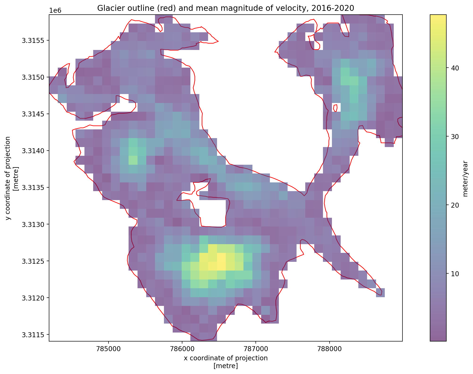
Now let’s take a look at the x and y components of velocity, again averaging over time:
fig, axs = plt.subplots(ncols =2, figsize=(17,7))
x = sample_glacier_raster.vx.mean(dim='mid_date').plot(ax=axs[0])
y = sample_glacier_raster.vy.mean(dim='mid_date').plot(ax=axs[1])
axs[0].set_title('x-component velocity')
axs[1].set_title('y-component velocity')
fig.suptitle('Temporal mean of velocity components')
x.colorbar.set_label('m/y', rotation=270)
y.colorbar.set_label('m/yr', rotation=270);
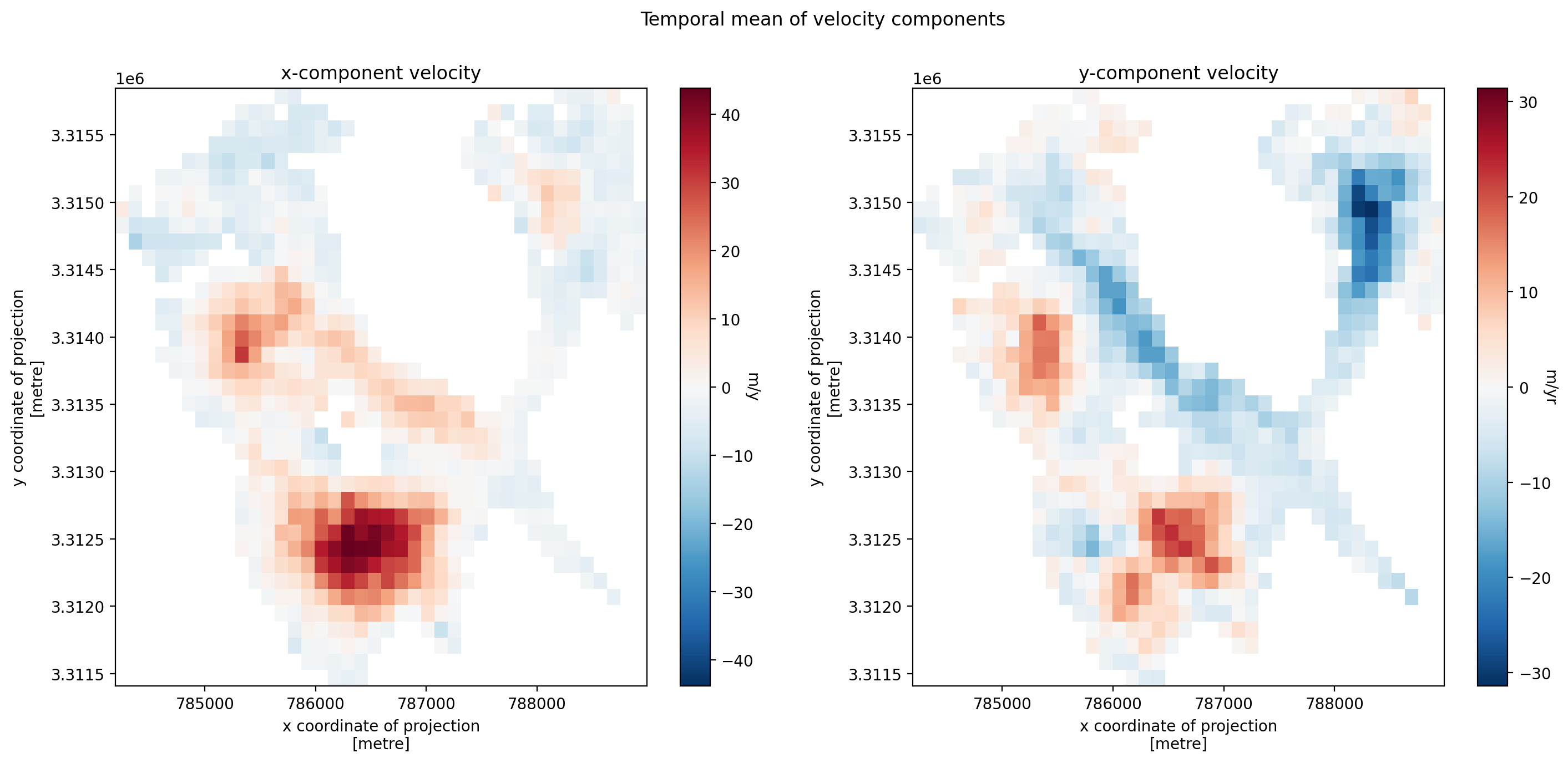
We can also plot the estimated error associated with the magnitude of velocity variable, which is included in the dataset
sample_glacier_raster.v_error.mean(dim=['mid_date']).plot();
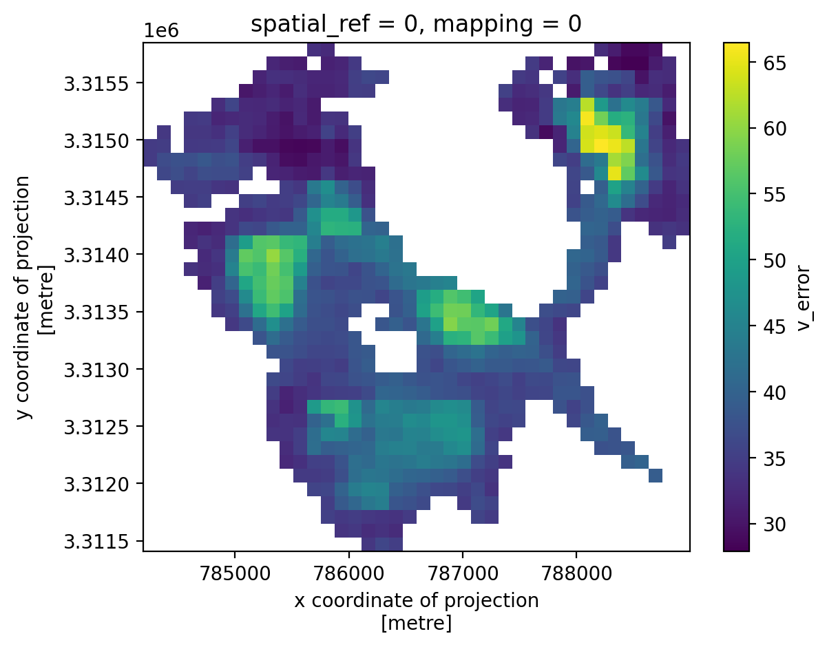
v_error is large relative to the velocity vectors, suggesting that this data could be pretty noisy.
Next we will visualize the velocity vectors.
fig, (ax,ax1)= plt.subplots(ncols=2, figsize=(20,9))
sample_glacier_vec.plot(ax=ax, facecolor='none', edgecolor='red')
sample_glacier_raster_timemean.plot.quiver('x','y','vx','vy', ax=ax, angles='xy', vmax=45, vmin=5, scale_units='xy', scale=1)
sample_glacier_vec.plot(ax=ax1, facecolor='none', edgecolor='red')
a = np.sqrt(sample_glacier_raster_timemean.vx**2 + sample_glacier_raster_timemean.vy**2).plot(ax=ax1, alpha=0.6, vmax=45, vmin=5)
a.colorbar.set_label('meter/year')
ax1.set_title('Glacier outline (red) and mean magnitude of velocity, 2016-2020');
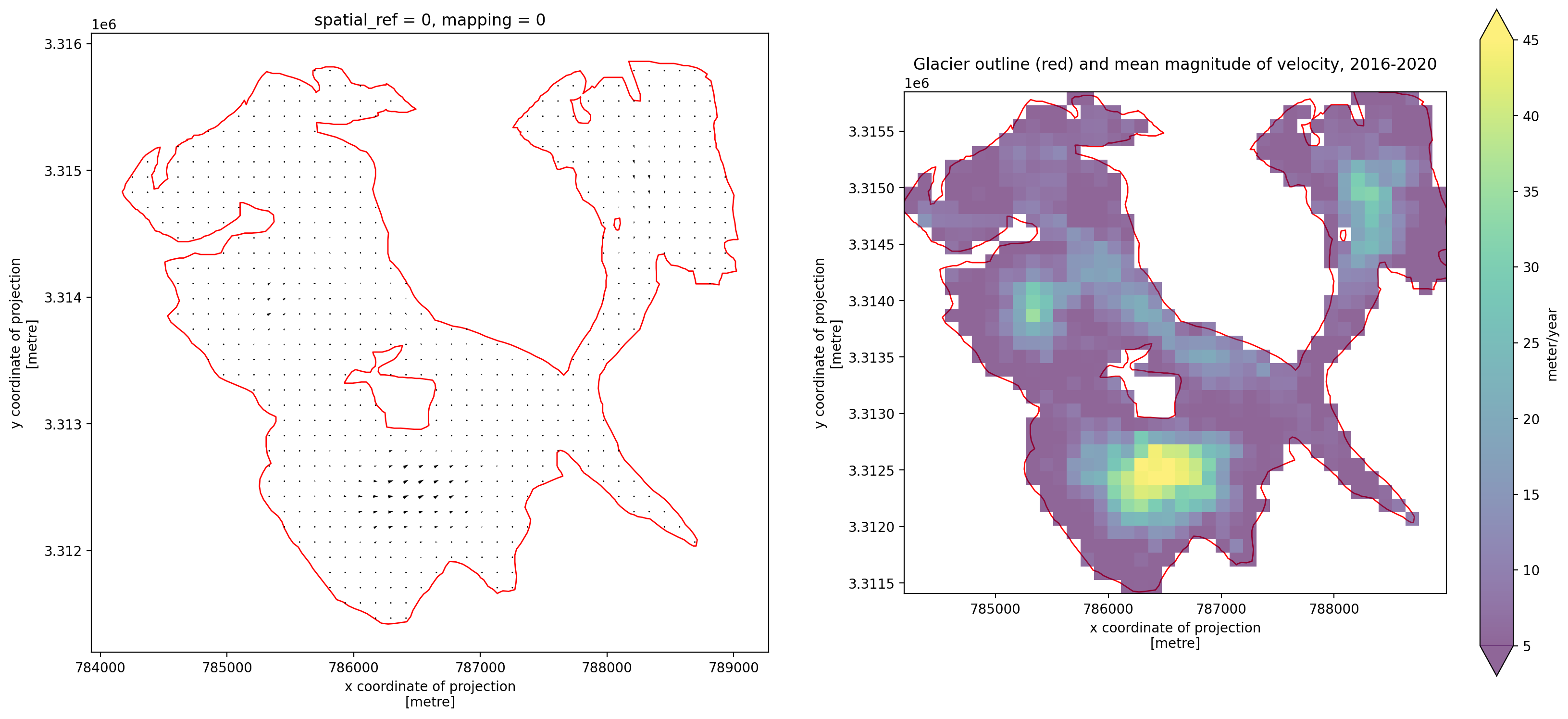
In this quiver plot, the units scale is set so that the horizontal and vertical components of velocity have the same units as the x and y dimensions (meters). This obscures a lot of the variability so we will replot the vectors letting the length be scaled based on average vector length
fig, (ax,ax1)= plt.subplots(ncols=2, figsize=(20,9))
sample_glacier_vec.plot(ax=ax, facecolor='none', edgecolor='red')
sample_glacier_raster_timemean.plot.quiver('x','y','vx','vy', ax=ax, angles='xy', vmax=45, vmin=5)
sample_glacier_vec.plot(ax=ax1, facecolor='none', edgecolor='red')
a = np.sqrt(sample_glacier_raster_timemean.vx**2 + sample_glacier_raster_timemean.vy**2).plot(ax=ax1, alpha=0.6)#, vmax=45, vmin=5)
a.colorbar.set_label('meter/year')
ax1.set_title('Glacier outline (red) and mean magnitude of velocity, 2016-2020');
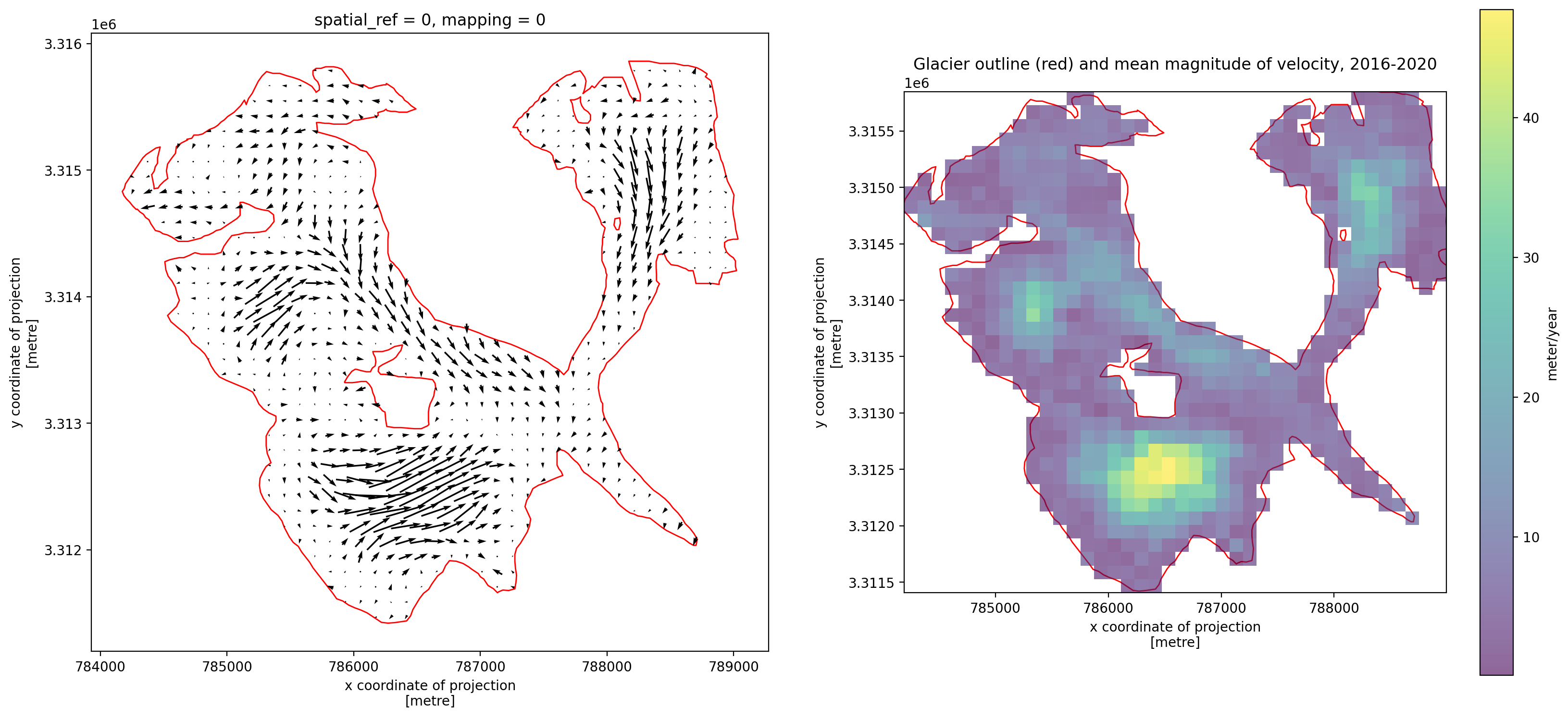
Now we can see more of the variability that aligns better with the calculated magnitude of velocity.
Exploring ITS_LIVE data#
ITS_LIVE data cubes come with many variables that carry information about the estimated surface velocities and the satellite images that were used to generate the surface velocity estimates. We won’t examine all of this information here but let’s look at a little bit.
To start with, let’s look at the satellite imagery used to generate the velocity data.
We see that we have two data_vars that indicate which sensor that each image in the image pair at a certain time step comes from.
sample_glacier_raster.satellite_img2
<xarray.DataArray 'satellite_img2' (mid_date: 3974)> Size: 32kB
array(['2B', '2B', '2B', ..., '8', '8', '7'], shape=(3974,), dtype=object)
Coordinates:
* mid_date (mid_date) datetime64[ns] 32kB 2018-04-14T04:18:49.171219968...
spatial_ref int64 8B 0
mapping int64 8B 0
Attributes:
description: id of the satellite that acquired image 2
standard_name: image2_satellite- mid_date: 3974
- '2B' '2B' '2B' '2A' '2A' '2B' '2B' ... '8' '8' '7' '7' '8' '8' '7'
array(['2B', '2B', '2B', ..., '8', '8', '7'], shape=(3974,), dtype=object)
- mid_date(mid_date)datetime64[ns]2018-04-14T04:18:49.171219968 .....
- description :
- midpoint of image 1 and image 2 acquisition date and time with granule's centroid longitude and latitude as microseconds
- standard_name :
- image_pair_center_date_with_time_separation
array(['2018-04-14T04:18:49.171219968', '2017-02-10T16:15:50.660901120', '2019-03-15T04:15:44.180925952', ..., '2018-06-11T04:10:57.953189888', '2017-05-27T04:10:08.145324032', '2017-05-07T04:11:30.865388288'], shape=(3974,), dtype='datetime64[ns]') - spatial_ref()int640
- GeoTransform :
- 784192.5 120.0 0.0 3315847.5 0.0 -120.0
array(0)
- mapping()int640
- crs_wkt :
- PROJCS["WGS 84 / UTM zone 46N",GEOGCS["WGS 84",DATUM["WGS_1984",SPHEROID["WGS 84",6378137,298.257223563,AUTHORITY["EPSG","7030"]],AUTHORITY["EPSG","6326"]],PRIMEM["Greenwich",0,AUTHORITY["EPSG","8901"]],UNIT["degree",0.0174532925199433,AUTHORITY["EPSG","9122"]],AUTHORITY["EPSG","4326"]],PROJECTION["Transverse_Mercator"],PARAMETER["latitude_of_origin",0],PARAMETER["central_meridian",93],PARAMETER["scale_factor",0.9996],PARAMETER["false_easting",500000],PARAMETER["false_northing",0],UNIT["metre",1,AUTHORITY["EPSG","9001"]],AXIS["Easting",EAST],AXIS["Northing",NORTH],AUTHORITY["EPSG","32646"]]
- semi_major_axis :
- 6378137.0
- semi_minor_axis :
- 6356752.314245179
- inverse_flattening :
- 298.257223563
- reference_ellipsoid_name :
- WGS 84
- longitude_of_prime_meridian :
- 0.0
- prime_meridian_name :
- Greenwich
- geographic_crs_name :
- WGS 84
- horizontal_datum_name :
- World Geodetic System 1984
- projected_crs_name :
- WGS 84 / UTM zone 46N
- grid_mapping_name :
- transverse_mercator
- latitude_of_projection_origin :
- 0.0
- longitude_of_central_meridian :
- 93.0
- false_easting :
- 500000.0
- false_northing :
- 0.0
- scale_factor_at_central_meridian :
- 0.9996
- spatial_ref :
- PROJCS["WGS 84 / UTM zone 46N",GEOGCS["WGS 84",DATUM["WGS_1984",SPHEROID["WGS 84",6378137,298.257223563,AUTHORITY["EPSG","7030"]],AUTHORITY["EPSG","6326"]],PRIMEM["Greenwich",0,AUTHORITY["EPSG","8901"]],UNIT["degree",0.0174532925199433,AUTHORITY["EPSG","9122"]],AUTHORITY["EPSG","4326"]],PROJECTION["Transverse_Mercator"],PARAMETER["latitude_of_origin",0],PARAMETER["central_meridian",93],PARAMETER["scale_factor",0.9996],PARAMETER["false_easting",500000],PARAMETER["false_northing",0],UNIT["metre",1,AUTHORITY["EPSG","9001"]],AXIS["Easting",EAST],AXIS["Northing",NORTH],AUTHORITY["EPSG","32646"]]
- GeoTransform :
- 784192.5 120.0 0.0 3315847.5 0.0 -120.0
array(0)
- mid_datePandasIndex
PandasIndex(DatetimeIndex(['2018-04-14 04:18:49.171219968', '2017-02-10 16:15:50.660901120', '2019-03-15 04:15:44.180925952', '2019-07-20 16:15:55.190603008', '2018-01-31 16:15:50.170811904', '2017-12-17 16:15:50.170508800', '2017-10-16 04:18:49.170811904', '2017-11-27 16:20:45.171105024', '2017-10-08 16:17:55.170906112', '2019-10-23 16:18:15.191001088', ... '2017-10-06 04:11:40.987761920', '2018-03-31 04:10:01.464065024', '2018-06-11 04:09:32.921265664', '2017-07-26 04:11:49.029760256', '2017-04-21 04:11:32.560144896', '2017-09-12 04:11:46.053865984', '2017-06-24 04:11:18.708142080', '2018-06-11 04:10:57.953189888', '2017-05-27 04:10:08.145324032', '2017-05-07 04:11:30.865388288'], dtype='datetime64[ns]', name='mid_date', length=3974, freq=None))
- description :
- id of the satellite that acquired image 2
- standard_name :
- image2_satellite
The satellite_img1 and satellite_img2 variables are 1-dimensional numpy arrays corresponding to the length of the mid_date dimension of the data cube. You can see that each element of the array is a string corresponding to a different satellite:
1A = Sentinel 1A, 1B = Sentinel 1B, 2A = Sentinel 2A
2B = Sentinel 2B, 7 = Landsat7, 8 = Landsat8
Examining velocity data from each satellite in ITS_LIVE dataset#
What if we only wanted to look at the velocity estimates from Landsat8?
l8_data = sample_glacier_raster.where(sample_glacier_raster['satellite_img1'] == '8', drop=True)
l8_data
<xarray.Dataset> Size: 51MB
Dimensions: (mid_date: 662, y: 37, x: 40)
Coordinates:
* mid_date (mid_date) datetime64[ns] 5kB 2017-12-25T04:1...
* x (x) float64 320B 7.843e+05 ... 7.889e+05
* y (y) float64 296B 3.316e+06 ... 3.311e+06
spatial_ref int64 8B 0
mapping int64 8B 0
Data variables: (12/59)
M11 (mid_date, y, x) float32 4MB nan nan ... nan nan
M11_dr_to_vr_factor (mid_date) float32 3kB nan nan nan ... nan nan
M12 (mid_date, y, x) float32 4MB nan nan ... nan nan
M12_dr_to_vr_factor (mid_date) float32 3kB nan nan nan ... nan nan
acquisition_date_img1 (mid_date) datetime64[ns] 5kB 2017-12-21T04:1...
acquisition_date_img2 (mid_date) datetime64[ns] 5kB 2017-12-29T04:1...
... ...
vy_error_modeled (mid_date) float32 3kB 1.163e+03 232.7 ... 166.2
vy_error_slow (mid_date) float32 3kB 112.5 37.6 ... 11.3 25.4
vy_error_stationary (mid_date) float32 3kB 112.5 37.6 ... 11.3 25.4
vy_stable_shift (mid_date) float32 3kB -74.2 -25.7 ... -10.8
vy_stable_shift_slow (mid_date) float32 3kB -73.8 -25.7 ... -10.7
vy_stable_shift_stationary (mid_date) float32 3kB -74.2 -25.7 ... -10.8
Attributes: (12/19)
Conventions: CF-1.8
GDAL_AREA_OR_POINT: Area
author: ITS_LIVE, a NASA MEaSUREs project (its-live.j...
autoRIFT_parameter_file: http://its-live-data.s3.amazonaws.com/autorif...
datacube_software_version: 1.0
date_created: 25-Sep-2023 22:00:23
... ...
s3: s3://its-live-data/datacubes/v2/N30E090/ITS_L...
skipped_granules: s3://its-live-data/datacubes/v2/N30E090/ITS_L...
time_standard_img1: UTC
time_standard_img2: UTC
title: ITS_LIVE datacube of image pair velocities
url: https://its-live-data.s3.amazonaws.com/datacu...- mid_date: 662
- y: 37
- x: 40
- mid_date(mid_date)datetime64[ns]2017-12-25T04:11:40.527109888 .....
- description :
- midpoint of image 1 and image 2 acquisition date and time with granule's centroid longitude and latitude as microseconds
- standard_name :
- image_pair_center_date_with_time_separation
array(['2017-12-25T04:11:40.527109888', '2018-12-12T04:08:03.179142912', '2018-12-04T04:08:17.320696064', ..., '2017-06-24T04:11:18.708142080', '2017-05-27T04:10:08.145324032', '2017-05-07T04:11:30.865388288'], shape=(662,), dtype='datetime64[ns]') - x(x)float647.843e+05 7.844e+05 ... 7.889e+05
- description :
- x coordinate of projection
- standard_name :
- projection_x_coordinate
- axis :
- X
- long_name :
- x coordinate of projection
- units :
- metre
array([784252.5, 784372.5, 784492.5, 784612.5, 784732.5, 784852.5, 784972.5, 785092.5, 785212.5, 785332.5, 785452.5, 785572.5, 785692.5, 785812.5, 785932.5, 786052.5, 786172.5, 786292.5, 786412.5, 786532.5, 786652.5, 786772.5, 786892.5, 787012.5, 787132.5, 787252.5, 787372.5, 787492.5, 787612.5, 787732.5, 787852.5, 787972.5, 788092.5, 788212.5, 788332.5, 788452.5, 788572.5, 788692.5, 788812.5, 788932.5]) - y(y)float643.316e+06 3.316e+06 ... 3.311e+06
- description :
- y coordinate of projection
- standard_name :
- projection_y_coordinate
- axis :
- Y
- long_name :
- y coordinate of projection
- units :
- metre
array([3315787.5, 3315667.5, 3315547.5, 3315427.5, 3315307.5, 3315187.5, 3315067.5, 3314947.5, 3314827.5, 3314707.5, 3314587.5, 3314467.5, 3314347.5, 3314227.5, 3314107.5, 3313987.5, 3313867.5, 3313747.5, 3313627.5, 3313507.5, 3313387.5, 3313267.5, 3313147.5, 3313027.5, 3312907.5, 3312787.5, 3312667.5, 3312547.5, 3312427.5, 3312307.5, 3312187.5, 3312067.5, 3311947.5, 3311827.5, 3311707.5, 3311587.5, 3311467.5]) - spatial_ref()int640
- GeoTransform :
- 784192.5 120.0 0.0 3315847.5 0.0 -120.0
array(0)
- mapping()int640
- crs_wkt :
- PROJCS["WGS 84 / UTM zone 46N",GEOGCS["WGS 84",DATUM["WGS_1984",SPHEROID["WGS 84",6378137,298.257223563,AUTHORITY["EPSG","7030"]],AUTHORITY["EPSG","6326"]],PRIMEM["Greenwich",0,AUTHORITY["EPSG","8901"]],UNIT["degree",0.0174532925199433,AUTHORITY["EPSG","9122"]],AUTHORITY["EPSG","4326"]],PROJECTION["Transverse_Mercator"],PARAMETER["latitude_of_origin",0],PARAMETER["central_meridian",93],PARAMETER["scale_factor",0.9996],PARAMETER["false_easting",500000],PARAMETER["false_northing",0],UNIT["metre",1,AUTHORITY["EPSG","9001"]],AXIS["Easting",EAST],AXIS["Northing",NORTH],AUTHORITY["EPSG","32646"]]
- semi_major_axis :
- 6378137.0
- semi_minor_axis :
- 6356752.314245179
- inverse_flattening :
- 298.257223563
- reference_ellipsoid_name :
- WGS 84
- longitude_of_prime_meridian :
- 0.0
- prime_meridian_name :
- Greenwich
- geographic_crs_name :
- WGS 84
- horizontal_datum_name :
- World Geodetic System 1984
- projected_crs_name :
- WGS 84 / UTM zone 46N
- grid_mapping_name :
- transverse_mercator
- latitude_of_projection_origin :
- 0.0
- longitude_of_central_meridian :
- 93.0
- false_easting :
- 500000.0
- false_northing :
- 0.0
- scale_factor_at_central_meridian :
- 0.9996
- spatial_ref :
- PROJCS["WGS 84 / UTM zone 46N",GEOGCS["WGS 84",DATUM["WGS_1984",SPHEROID["WGS 84",6378137,298.257223563,AUTHORITY["EPSG","7030"]],AUTHORITY["EPSG","6326"]],PRIMEM["Greenwich",0,AUTHORITY["EPSG","8901"]],UNIT["degree",0.0174532925199433,AUTHORITY["EPSG","9122"]],AUTHORITY["EPSG","4326"]],PROJECTION["Transverse_Mercator"],PARAMETER["latitude_of_origin",0],PARAMETER["central_meridian",93],PARAMETER["scale_factor",0.9996],PARAMETER["false_easting",500000],PARAMETER["false_northing",0],UNIT["metre",1,AUTHORITY["EPSG","9001"]],AXIS["Easting",EAST],AXIS["Northing",NORTH],AUTHORITY["EPSG","32646"]]
- GeoTransform :
- 784192.5 120.0 0.0 3315847.5 0.0 -120.0
array(0)
- M11(mid_date, y, x)float32nan nan nan nan ... nan nan nan nan
- description :
- conversion matrix element (1st row, 1st column) that can be multiplied with vx to give range pixel displacement dr (see Eq. A18 in https://www.mdpi.com/2072-4292/13/4/749)
- standard_name :
- conversion_matrix_element_11
- units :
- pixel/(meter/year)
array([[[nan, nan, nan, ..., nan, nan, nan], [nan, nan, nan, ..., nan, nan, nan], [nan, nan, nan, ..., nan, nan, nan], ..., [nan, nan, nan, ..., nan, nan, nan], [nan, nan, nan, ..., nan, nan, nan], [nan, nan, nan, ..., nan, nan, nan]], [[nan, nan, nan, ..., nan, nan, nan], [nan, nan, nan, ..., nan, nan, nan], [nan, nan, nan, ..., nan, nan, nan], ..., [nan, nan, nan, ..., nan, nan, nan], [nan, nan, nan, ..., nan, nan, nan], [nan, nan, nan, ..., nan, nan, nan]], [[nan, nan, nan, ..., nan, nan, nan], [nan, nan, nan, ..., nan, nan, nan], [nan, nan, nan, ..., nan, nan, nan], ..., ... [nan, nan, nan, ..., nan, nan, nan], [nan, nan, nan, ..., nan, nan, nan], [nan, nan, nan, ..., nan, nan, nan]], [[nan, nan, nan, ..., nan, nan, nan], [nan, nan, nan, ..., nan, nan, nan], [nan, nan, nan, ..., nan, nan, nan], ..., [nan, nan, nan, ..., nan, nan, nan], [nan, nan, nan, ..., nan, nan, nan], [nan, nan, nan, ..., nan, nan, nan]], [[nan, nan, nan, ..., nan, nan, nan], [nan, nan, nan, ..., nan, nan, nan], [nan, nan, nan, ..., nan, nan, nan], ..., [nan, nan, nan, ..., nan, nan, nan], [nan, nan, nan, ..., nan, nan, nan], [nan, nan, nan, ..., nan, nan, nan]]], shape=(662, 37, 40), dtype=float32) - M11_dr_to_vr_factor(mid_date)float32nan nan nan nan ... nan nan nan nan
- description :
- multiplicative factor that converts slant range pixel displacement dr to slant range velocity vr
- standard_name :
- M11_dr_to_vr_factor
- units :
- meter/(year*pixel)
array([nan, nan, nan, nan, nan, nan, nan, nan, nan, nan, nan, nan, nan, nan, nan, nan, nan, nan, nan, nan, nan, nan, nan, nan, nan, nan, nan, nan, nan, nan, nan, nan, nan, nan, nan, nan, nan, nan, nan, nan, nan, nan, nan, nan, nan, nan, nan, nan, nan, nan, nan, nan, nan, nan, nan, nan, nan, nan, nan, nan, nan, nan, nan, nan, nan, nan, nan, nan, nan, nan, nan, nan, nan, nan, nan, nan, nan, nan, nan, nan, nan, nan, nan, nan, nan, nan, nan, nan, nan, nan, nan, nan, nan, nan, nan, nan, nan, nan, nan, nan, nan, nan, nan, nan, nan, nan, nan, nan, nan, nan, nan, nan, nan, nan, nan, nan, nan, nan, nan, nan, nan, nan, nan, nan, nan, nan, nan, nan, nan, nan, nan, nan, nan, nan, nan, nan, nan, nan, nan, nan, nan, nan, nan, nan, nan, nan, nan, nan, nan, nan, nan, nan, nan, nan, nan, nan, nan, nan, nan, nan, nan, nan, nan, nan, nan, nan, nan, nan, nan, nan, nan, nan, nan, nan, nan, nan, nan, nan, nan, nan, nan, nan, nan, nan, nan, nan, nan, nan, nan, nan, nan, nan, nan, nan, nan, nan, nan, nan, nan, nan, nan, nan, nan, nan, nan, nan, nan, nan, nan, nan, nan, nan, nan, nan, nan, nan, nan, nan, nan, nan, nan, nan, nan, nan, nan, nan, nan, nan, nan, nan, nan, nan, nan, nan, nan, nan, nan, nan, nan, nan, nan, nan, nan, nan, nan, nan, nan, nan, nan, nan, nan, nan, nan, nan, nan, nan, nan, nan, nan, nan, ... nan, nan, nan, nan, nan, nan, nan, nan, nan, nan, nan, nan, nan, nan, nan, nan, nan, nan, nan, nan, nan, nan, nan, nan, nan, nan, nan, nan, nan, nan, nan, nan, nan, nan, nan, nan, nan, nan, nan, nan, nan, nan, nan, nan, nan, nan, nan, nan, nan, nan, nan, nan, nan, nan, nan, nan, nan, nan, nan, nan, nan, nan, nan, nan, nan, nan, nan, nan, nan, nan, nan, nan, nan, nan, nan, nan, nan, nan, nan, nan, nan, nan, nan, nan, nan, nan, nan, nan, nan, nan, nan, nan, nan, nan, nan, nan, nan, nan, nan, nan, nan, nan, nan, nan, nan, nan, nan, nan, nan, nan, nan, nan, nan, nan, nan, nan, nan, nan, nan, nan, nan, nan, nan, nan, nan, nan, nan, nan, nan, nan, nan, nan, nan, nan, nan, nan, nan, nan, nan, nan, nan, nan, nan, nan, nan, nan, nan, nan, nan, nan, nan, nan, nan, nan, nan, nan, nan, nan, nan, nan, nan, nan, nan, nan, nan, nan, nan, nan, nan, nan, nan, nan, nan, nan, nan, nan, nan, nan, nan, nan, nan, nan, nan, nan, nan, nan, nan, nan, nan, nan, nan, nan, nan, nan, nan, nan, nan, nan, nan, nan, nan, nan, nan, nan, nan, nan, nan, nan, nan, nan, nan, nan, nan, nan, nan, nan, nan, nan, nan, nan, nan, nan, nan, nan, nan, nan, nan, nan, nan, nan, nan, nan, nan, nan, nan, nan, nan, nan, nan, nan, nan, nan, nan, nan, nan, nan], dtype=float32) - M12(mid_date, y, x)float32nan nan nan nan ... nan nan nan nan
- description :
- conversion matrix element (1st row, 2nd column) that can be multiplied with vy to give range pixel displacement dr (see Eq. A18 in https://www.mdpi.com/2072-4292/13/4/749)
- standard_name :
- conversion_matrix_element_12
- units :
- pixel/(meter/year)
array([[[nan, nan, nan, ..., nan, nan, nan], [nan, nan, nan, ..., nan, nan, nan], [nan, nan, nan, ..., nan, nan, nan], ..., [nan, nan, nan, ..., nan, nan, nan], [nan, nan, nan, ..., nan, nan, nan], [nan, nan, nan, ..., nan, nan, nan]], [[nan, nan, nan, ..., nan, nan, nan], [nan, nan, nan, ..., nan, nan, nan], [nan, nan, nan, ..., nan, nan, nan], ..., [nan, nan, nan, ..., nan, nan, nan], [nan, nan, nan, ..., nan, nan, nan], [nan, nan, nan, ..., nan, nan, nan]], [[nan, nan, nan, ..., nan, nan, nan], [nan, nan, nan, ..., nan, nan, nan], [nan, nan, nan, ..., nan, nan, nan], ..., ... [nan, nan, nan, ..., nan, nan, nan], [nan, nan, nan, ..., nan, nan, nan], [nan, nan, nan, ..., nan, nan, nan]], [[nan, nan, nan, ..., nan, nan, nan], [nan, nan, nan, ..., nan, nan, nan], [nan, nan, nan, ..., nan, nan, nan], ..., [nan, nan, nan, ..., nan, nan, nan], [nan, nan, nan, ..., nan, nan, nan], [nan, nan, nan, ..., nan, nan, nan]], [[nan, nan, nan, ..., nan, nan, nan], [nan, nan, nan, ..., nan, nan, nan], [nan, nan, nan, ..., nan, nan, nan], ..., [nan, nan, nan, ..., nan, nan, nan], [nan, nan, nan, ..., nan, nan, nan], [nan, nan, nan, ..., nan, nan, nan]]], shape=(662, 37, 40), dtype=float32) - M12_dr_to_vr_factor(mid_date)float32nan nan nan nan ... nan nan nan nan
- description :
- multiplicative factor that converts slant range pixel displacement dr to slant range velocity vr
- standard_name :
- M12_dr_to_vr_factor
- units :
- meter/(year*pixel)
array([nan, nan, nan, nan, nan, nan, nan, nan, nan, nan, nan, nan, nan, nan, nan, nan, nan, nan, nan, nan, nan, nan, nan, nan, nan, nan, nan, nan, nan, nan, nan, nan, nan, nan, nan, nan, nan, nan, nan, nan, nan, nan, nan, nan, nan, nan, nan, nan, nan, nan, nan, nan, nan, nan, nan, nan, nan, nan, nan, nan, nan, nan, nan, nan, nan, nan, nan, nan, nan, nan, nan, nan, nan, nan, nan, nan, nan, nan, nan, nan, nan, nan, nan, nan, nan, nan, nan, nan, nan, nan, nan, nan, nan, nan, nan, nan, nan, nan, nan, nan, nan, nan, nan, nan, nan, nan, nan, nan, nan, nan, nan, nan, nan, nan, nan, nan, nan, nan, nan, nan, nan, nan, nan, nan, nan, nan, nan, nan, nan, nan, nan, nan, nan, nan, nan, nan, nan, nan, nan, nan, nan, nan, nan, nan, nan, nan, nan, nan, nan, nan, nan, nan, nan, nan, nan, nan, nan, nan, nan, nan, nan, nan, nan, nan, nan, nan, nan, nan, nan, nan, nan, nan, nan, nan, nan, nan, nan, nan, nan, nan, nan, nan, nan, nan, nan, nan, nan, nan, nan, nan, nan, nan, nan, nan, nan, nan, nan, nan, nan, nan, nan, nan, nan, nan, nan, nan, nan, nan, nan, nan, nan, nan, nan, nan, nan, nan, nan, nan, nan, nan, nan, nan, nan, nan, nan, nan, nan, nan, nan, nan, nan, nan, nan, nan, nan, nan, nan, nan, nan, nan, nan, nan, nan, nan, nan, nan, nan, nan, nan, nan, nan, nan, nan, nan, nan, nan, nan, nan, nan, nan, ... nan, nan, nan, nan, nan, nan, nan, nan, nan, nan, nan, nan, nan, nan, nan, nan, nan, nan, nan, nan, nan, nan, nan, nan, nan, nan, nan, nan, nan, nan, nan, nan, nan, nan, nan, nan, nan, nan, nan, nan, nan, nan, nan, nan, nan, nan, nan, nan, nan, nan, nan, nan, nan, nan, nan, nan, nan, nan, nan, nan, nan, nan, nan, nan, nan, nan, nan, nan, nan, nan, nan, nan, nan, nan, nan, nan, nan, nan, nan, nan, nan, nan, nan, nan, nan, nan, nan, nan, nan, nan, nan, nan, nan, nan, nan, nan, nan, nan, nan, nan, nan, nan, nan, nan, nan, nan, nan, nan, nan, nan, nan, nan, nan, nan, nan, nan, nan, nan, nan, nan, nan, nan, nan, nan, nan, nan, nan, nan, nan, nan, nan, nan, nan, nan, nan, nan, nan, nan, nan, nan, nan, nan, nan, nan, nan, nan, nan, nan, nan, nan, nan, nan, nan, nan, nan, nan, nan, nan, nan, nan, nan, nan, nan, nan, nan, nan, nan, nan, nan, nan, nan, nan, nan, nan, nan, nan, nan, nan, nan, nan, nan, nan, nan, nan, nan, nan, nan, nan, nan, nan, nan, nan, nan, nan, nan, nan, nan, nan, nan, nan, nan, nan, nan, nan, nan, nan, nan, nan, nan, nan, nan, nan, nan, nan, nan, nan, nan, nan, nan, nan, nan, nan, nan, nan, nan, nan, nan, nan, nan, nan, nan, nan, nan, nan, nan, nan, nan, nan, nan, nan, nan, nan, nan, nan, nan, nan], dtype=float32) - acquisition_date_img1(mid_date)datetime64[ns]2017-12-21T04:10:40.253580032 .....
- description :
- acquisition date and time of image 1
- standard_name :
- image1_acquition_date
array(['2017-12-21T04:10:40.253580032', '2018-11-22T04:10:24.234354944', '2018-11-22T04:10:24.234354944', '2017-02-04T04:10:29.099783936', '2018-01-22T04:10:27.510945024', '2018-11-22T04:10:24.234354944', '2017-01-19T04:10:36.447260928', '2017-02-04T04:10:29.099783936', '2017-11-03T04:10:45.832015872', '2017-11-03T04:10:45.832015872', '2017-02-04T04:10:29.099783936', '2017-12-21T04:10:40.253580032', '2018-11-22T04:10:24.234354944', '2018-01-22T04:10:27.510945024', '2018-11-22T04:10:24.234354944', '2017-12-21T04:10:40.253580032', '2017-02-04T04:10:29.099783936', '2017-01-19T04:10:36.447260928', '2018-01-22T04:10:27.510945024', '2017-01-19T04:10:36.447260928', '2017-02-04T04:10:29.099783936', '2017-02-04T04:10:29.099783936', '2018-01-22T04:10:27.510945024', '2017-11-03T04:10:45.832015872', '2017-11-03T04:10:45.832015872', '2018-12-08T04:10:21.702228992', '2017-02-04T04:10:29.099783936', '2018-01-22T04:10:27.510945024', '2016-10-31T04:10:49.197186048', '2018-01-22T04:10:27.510945024', '2016-10-31T04:10:49.197186048', '2017-01-19T04:10:36.447260928', '2018-12-08T04:10:21.702228992', '2017-01-19T04:10:36.447260928', '2017-12-21T04:10:40.253580032', '2017-11-03T04:10:45.832015872', '2017-12-21T04:10:40.253580032', '2017-01-19T04:10:36.447260928', '2018-01-22T04:10:27.510945024', '2019-01-09T04:10:19.605915904', ... '2017-07-30T04:10:25.156854016', '2017-07-30T04:10:25.156854016', '2017-07-30T04:10:25.156854016', '2017-07-30T04:10:25.156854016', '2018-02-07T04:10:19.247780096', '2016-11-16T04:10:48.428282112', '2016-10-15T04:10:47.896870912', '2017-07-30T04:10:25.156854016', '2018-03-27T04:09:57.437323008', '2017-07-30T04:10:25.156854016', '2017-04-09T04:09:59.003422976', '2018-02-07T04:10:19.247780096', '2017-04-09T04:09:59.003422976', '2016-10-15T04:10:47.896870912', '2017-07-30T04:10:25.156854016', '2017-07-30T04:10:25.156854016', '2017-07-30T04:10:25.156854016', '2017-09-16T04:10:35.331774976', '2017-10-18T04:10:46.076395008', '2017-07-30T04:10:25.156854016', '2016-10-15T04:10:47.896870912', '2017-11-19T04:10:41.686725376', '2017-04-09T04:09:59.003422976', '2018-05-30T04:09:17.034597888', '2017-04-09T04:09:59.003422976', '2017-07-14T04:10:16.946407936', '2017-04-09T04:09:59.003422976', '2017-09-16T04:10:35.331774976', '2017-07-30T04:10:25.156854016', '2018-05-14T04:09:29.903631104', '2017-09-16T04:10:35.331774976', '2017-09-16T04:10:35.331774976', '2017-12-05T04:10:37.029957888', '2018-04-28T04:09:39.925913088', '2017-07-30T04:10:25.156854016', '2016-10-15T04:10:47.896870912', '2017-04-09T04:09:59.003422976', '2017-04-09T04:09:59.003422976'], dtype='datetime64[ns]') - acquisition_date_img2(mid_date)datetime64[ns]2017-12-29T04:12:40.458198016 .....
- description :
- acquisition date and time of image 2
- standard_name :
- image2_acquition_date
array(['2017-12-29T04:12:40.458198016', '2019-01-01T04:05:41.761686272', '2018-12-16T04:06:10.044793088', '2017-12-29T04:12:40.458198016', '2019-01-01T04:05:41.761686272', '2020-02-13T04:10:30.639724032', '2017-01-27T04:12:29.455911936', '2018-01-22T04:10:27.510945024', '2017-11-11T04:13:04.720666112', '2017-12-29T04:12:40.458198016', '2018-02-15T04:11:59.198033920', '2019-01-01T04:05:41.761686272', '2019-01-17T04:05:11.586401024', '2018-12-16T04:06:10.044793088', '2018-11-30T04:06:36.228204288', '2018-12-16T04:06:10.044793088', '2017-12-21T04:10:40.253580032', '2017-12-29T04:12:40.458198016', '2018-02-15T04:11:59.198033920', '2018-01-22T04:10:27.510945024', '2017-11-11T04:13:04.720666112', '2017-02-28T04:12:32.528041984', '2018-11-22T04:10:24.234354944', '2018-01-22T04:10:27.510945024', '2017-12-21T04:10:40.253580032', '2019-01-01T04:05:41.761686272', '2017-11-03T04:10:45.832015872', '2019-06-02T04:10:12.332978176', '2017-11-11T04:13:04.720666112', '2019-01-17T04:05:11.586401024', '2017-12-29T04:12:40.458198016', '2017-12-21T04:10:40.253580032', '2018-12-16T04:06:10.044793088', '2018-02-15T04:11:59.198033920', '2019-06-02T04:10:12.332978176', '2019-01-01T04:05:41.761686272', '2018-02-15T04:11:59.198033920', '2017-02-28T04:12:32.528041984', '2018-11-30T04:06:36.228204288', '2020-02-29T04:10:26.243158016', ... '2017-11-19T04:10:41.686725376', '2018-05-30T04:09:17.034597888', '2018-01-30T04:12:11.667300096', '2018-04-04T04:11:23.527504896', '2018-03-03T04:11:49.197383936', '2018-03-03T04:11:49.197383936', '2017-06-04T04:13:02.386535936', '2018-11-30T04:06:36.228204288', '2018-07-25T04:09:25.555763200', '2018-05-22T04:10:35.049019904', '2018-05-22T04:10:35.049019904', '2018-10-29T04:07:21.963168256', '2017-10-26T04:13:06.609417984', '2017-04-09T04:09:59.003422976', '2019-01-25T04:10:15.711925760', '2018-01-14T04:12:27.084400896', '2019-01-09T04:10:19.605915904', '2017-10-26T04:13:06.609417984', '2018-03-03T04:11:49.197383936', '2018-07-25T04:09:25.555763200', '2017-07-14T04:10:16.946407936', '2018-07-25T04:09:25.555763200', '2018-03-03T04:11:49.197383936', '2018-07-25T04:09:25.555763200', '2018-09-19T04:10:06.348390144', '2017-10-26T04:13:06.609417984', '2017-09-16T04:10:35.331774976', '2018-11-30T04:06:36.228204288', '2018-10-29T04:07:21.963168256', '2018-07-25T04:09:25.555763200', '2018-10-29T04:07:21.963168256', '2018-03-03T04:11:49.197383936', '2018-07-25T04:09:25.555763200', '2018-07-25T04:09:25.555763200', '2017-10-26T04:13:06.609417984', '2018-03-03T04:11:49.197383936', '2017-07-14T04:10:16.946407936', '2017-06-04T04:13:02.386535936'], dtype='datetime64[ns]') - autoRIFT_software_version(mid_date)object'1.5.0' '1.5.0' ... '1.5.0' '1.5.0'
- description :
- version of autoRIFT software
- standard_name :
- autoRIFT_software_version
array(['1.5.0', '1.5.0', '1.5.0', '1.5.0', '1.5.0', '1.5.0', '1.5.0', '1.5.0', '1.5.0', '1.5.0', '1.5.0', '1.5.0', '1.5.0', '1.5.0', '1.5.0', '1.5.0', '1.5.0', '1.5.0', '1.5.0', '1.5.0', '1.5.0', '1.5.0', '1.5.0', '1.5.0', '1.5.0', '1.5.0', '1.5.0', '1.5.0', '1.5.0', '1.5.0', '1.5.0', '1.5.0', '1.5.0', '1.5.0', '1.5.0', '1.5.0', '1.5.0', '1.5.0', '1.5.0', '1.5.0', '1.5.0', '1.5.0', '1.5.0', '1.5.0', '1.5.0', '1.5.0', '1.5.0', '1.5.0', '1.5.0', '1.5.0', '1.5.0', '1.5.0', '1.5.0', '1.5.0', '1.5.0', '1.5.0', '1.5.0', '1.5.0', '1.5.0', '1.5.0', '1.5.0', '1.5.0', '1.5.0', '1.5.0', '1.5.0', '1.5.0', '1.5.0', '1.5.0', '1.5.0', '1.5.0', '1.5.0', '1.5.0', '1.5.0', '1.5.0', '1.5.0', '1.5.0', '1.5.0', '1.5.0', '1.5.0', '1.5.0', '1.5.0', '1.5.0', '1.5.0', '1.5.0', '1.5.0', '1.5.0', '1.5.0', '1.5.0', '1.5.0', '1.5.0', '1.5.0', '1.5.0', '1.5.0', '1.5.0', '1.5.0', '1.5.0', '1.5.0', '1.5.0', '1.5.0', '1.5.0', '1.5.0', '1.5.0', '1.5.0', '1.5.0', '1.5.0', '1.5.0', '1.5.0', '1.5.0', '1.5.0', '1.5.0', '1.5.0', '1.5.0', '1.5.0', '1.5.0', '1.5.0', '1.5.0', '1.5.0', '1.5.0', '1.5.0', '1.5.0', '1.5.0', '1.5.0', '1.5.0', '1.5.0', '1.5.0', '1.5.0', '1.5.0', '1.5.0', '1.5.0', '1.5.0', '1.5.0', '1.5.0', '1.5.0', '1.5.0', '1.5.0', '1.5.0', '1.5.0', '1.5.0', '1.5.0', '1.5.0', ... '1.5.0', '1.5.0', '1.5.0', '1.5.0', '1.5.0', '1.5.0', '1.5.0', '1.5.0', '1.5.0', '1.5.0', '1.5.0', '1.5.0', '1.5.0', '1.5.0', '1.5.0', '1.5.0', '1.5.0', '1.5.0', '1.5.0', '1.5.0', '1.5.0', '1.5.0', '1.5.0', '1.5.0', '1.5.0', '1.5.0', '1.5.0', '1.5.0', '1.5.0', '1.5.0', '1.5.0', '1.5.0', '1.5.0', '1.5.0', '1.5.0', '1.5.0', '1.5.0', '1.5.0', '1.5.0', '1.5.0', '1.5.0', '1.5.0', '1.5.0', '1.5.0', '1.5.0', '1.5.0', '1.5.0', '1.5.0', '1.5.0', '1.5.0', '1.5.0', '1.5.0', '1.5.0', '1.5.0', '1.5.0', '1.5.0', '1.5.0', '1.5.0', '1.5.0', '1.5.0', '1.5.0', '1.5.0', '1.5.0', '1.5.0', '1.5.0', '1.5.0', '1.5.0', '1.5.0', '1.5.0', '1.5.0', '1.5.0', '1.5.0', '1.5.0', '1.5.0', '1.5.0', '1.5.0', '1.5.0', '1.5.0', '1.5.0', '1.5.0', '1.5.0', '1.5.0', '1.5.0', '1.5.0', '1.5.0', '1.5.0', '1.5.0', '1.5.0', '1.5.0', '1.5.0', '1.5.0', '1.5.0', '1.5.0', '1.5.0', '1.5.0', '1.5.0', '1.5.0', '1.5.0', '1.5.0', '1.5.0', '1.5.0', '1.5.0', '1.5.0', '1.5.0', '1.5.0', '1.5.0', '1.5.0', '1.5.0', '1.5.0', '1.5.0', '1.5.0', '1.5.0', '1.5.0', '1.5.0', '1.5.0', '1.5.0', '1.5.0', '1.5.0', '1.5.0', '1.5.0', '1.5.0', '1.5.0', '1.5.0', '1.5.0', '1.5.0', '1.5.0', '1.5.0', '1.5.0', '1.5.0', '1.5.0', '1.5.0', '1.5.0', '1.5.0', '1.5.0', '1.5.0', '1.5.0', '1.5.0'], dtype=object) - chip_size_height(mid_date, y, x)float32nan nan nan nan ... nan nan nan nan
- chip_size_coordinates :
- Optical data: chip_size_coordinates = 'image projection geometry: width = x, height = y'. Radar data: chip_size_coordinates = 'radar geometry: width = range, height = azimuth'
- description :
- height of search template (chip)
- standard_name :
- chip_size_height
- units :
- m
- y_pixel_size :
- 10.0
array([[[ nan, nan, nan, ..., 480., nan, nan], [ nan, nan, nan, ..., 480., 480., nan], [ nan, nan, nan, ..., 480., 480., nan], ..., [ nan, nan, nan, ..., nan, nan, nan], [ nan, nan, nan, ..., nan, nan, nan], [ nan, nan, nan, ..., nan, nan, nan]], [[ nan, nan, nan, ..., 480., nan, nan], [ nan, nan, nan, ..., 480., 480., nan], [ nan, nan, nan, ..., 480., 480., nan], ..., [ nan, nan, nan, ..., nan, nan, nan], [ nan, nan, nan, ..., nan, nan, nan], [ nan, nan, nan, ..., nan, nan, nan]], [[ nan, nan, nan, ..., 240., nan, nan], [ nan, nan, nan, ..., 480., 480., nan], [ nan, nan, nan, ..., 480., 480., nan], ..., ... [ nan, nan, nan, ..., nan, nan, nan], [ nan, nan, nan, ..., nan, nan, nan], [ nan, nan, nan, ..., nan, nan, nan]], [[ nan, nan, nan, ..., nan, nan, nan], [ nan, nan, nan, ..., nan, nan, nan], [ nan, nan, nan, ..., nan, nan, nan], ..., [ nan, nan, nan, ..., nan, nan, nan], [ nan, nan, nan, ..., nan, nan, nan], [ nan, nan, nan, ..., nan, nan, nan]], [[ nan, nan, nan, ..., nan, nan, nan], [ nan, nan, nan, ..., nan, nan, nan], [ nan, nan, nan, ..., nan, nan, nan], ..., [ nan, nan, nan, ..., nan, nan, nan], [ nan, nan, nan, ..., nan, nan, nan], [ nan, nan, nan, ..., nan, nan, nan]]], shape=(662, 37, 40), dtype=float32) - chip_size_width(mid_date, y, x)float32nan nan nan nan ... nan nan nan nan
- chip_size_coordinates :
- Optical data: chip_size_coordinates = 'image projection geometry: width = x, height = y'. Radar data: chip_size_coordinates = 'radar geometry: width = range, height = azimuth'
- description :
- width of search template (chip)
- standard_name :
- chip_size_width
- units :
- m
- x_pixel_size :
- 10.0
array([[[ nan, nan, nan, ..., 480., nan, nan], [ nan, nan, nan, ..., 480., 480., nan], [ nan, nan, nan, ..., 480., 480., nan], ..., [ nan, nan, nan, ..., nan, nan, nan], [ nan, nan, nan, ..., nan, nan, nan], [ nan, nan, nan, ..., nan, nan, nan]], [[ nan, nan, nan, ..., 480., nan, nan], [ nan, nan, nan, ..., 480., 480., nan], [ nan, nan, nan, ..., 480., 480., nan], ..., [ nan, nan, nan, ..., nan, nan, nan], [ nan, nan, nan, ..., nan, nan, nan], [ nan, nan, nan, ..., nan, nan, nan]], [[ nan, nan, nan, ..., 240., nan, nan], [ nan, nan, nan, ..., 480., 480., nan], [ nan, nan, nan, ..., 480., 480., nan], ..., ... [ nan, nan, nan, ..., nan, nan, nan], [ nan, nan, nan, ..., nan, nan, nan], [ nan, nan, nan, ..., nan, nan, nan]], [[ nan, nan, nan, ..., nan, nan, nan], [ nan, nan, nan, ..., nan, nan, nan], [ nan, nan, nan, ..., nan, nan, nan], ..., [ nan, nan, nan, ..., nan, nan, nan], [ nan, nan, nan, ..., nan, nan, nan], [ nan, nan, nan, ..., nan, nan, nan]], [[ nan, nan, nan, ..., nan, nan, nan], [ nan, nan, nan, ..., nan, nan, nan], [ nan, nan, nan, ..., nan, nan, nan], ..., [ nan, nan, nan, ..., nan, nan, nan], [ nan, nan, nan, ..., nan, nan, nan], [ nan, nan, nan, ..., nan, nan, nan]]], shape=(662, 37, 40), dtype=float32) - date_center(mid_date)datetime64[ns]2017-12-25T04:11:40.355888896 .....
- description :
- midpoint of image 1 and image 2 acquisition date
- standard_name :
- image_pair_center_date
array(['2017-12-25T04:11:40.355888896', '2018-12-12T04:08:02.998021120', '2018-12-04T04:08:17.139574016', '2017-07-18T04:11:34.778990848', '2018-07-13T04:08:04.636314880', '2019-07-04T04:10:27.437039104', '2017-01-23T04:11:32.951587072', '2017-07-30T04:10:28.305363968', '2017-11-07T04:11:55.276340992', '2017-12-01T04:11:43.145106944', '2017-08-11T04:11:14.148909056', '2018-06-27T04:08:11.007632896', '2018-12-20T04:07:47.910377984', '2018-07-05T04:08:18.777868800', '2018-11-26T04:08:30.231279104', '2018-06-19T04:08:25.149186048', '2017-07-14T04:10:34.676681984', '2017-07-10T04:11:38.452729088', '2018-02-03T04:11:13.354489088', '2017-07-22T04:10:31.979102976', '2017-06-24T04:11:46.910224896', '2017-02-16T04:11:30.813913088', '2018-06-23T04:10:25.872649728', '2017-12-13T04:10:36.671480064', '2017-11-27T04:10:43.042798080', '2018-12-20T04:08:01.731956992', '2017-06-20T04:10:37.465900032', '2018-09-27T04:10:19.921960960', '2017-05-07T04:11:56.958926336', '2018-07-21T04:07:49.548673024', '2017-05-31T04:11:44.827692032', '2017-07-06T04:10:38.350421248', '2018-12-12T04:08:15.873510912', '2017-08-03T04:11:17.822647296', '2018-09-11T04:10:26.293278976', '2018-06-03T04:08:13.796850944', '2018-01-18T04:11:19.725807104', '2017-02-08T04:11:34.487651328', '2018-06-27T04:08:31.869574912', '2019-08-05T04:10:22.924537088', ... '2017-09-24T04:10:33.421789952', '2017-12-29T04:09:51.095726336', '2017-10-30T04:11:18.412077056', '2017-12-01T04:10:54.342180096', '2018-02-19T04:11:04.222582016', '2017-07-10T04:11:18.812833024', '2017-02-08T04:11:55.141702912', '2018-03-31T04:08:30.692528640', '2018-05-26T04:09:41.496542976', '2017-12-25T04:10:30.102937088', '2017-10-30T04:10:17.026221056', '2018-06-19T04:08:50.605474048', '2017-07-18T04:11:32.806420992', '2017-01-11T04:10:23.450147072', '2018-04-28T04:10:20.434390016', '2017-10-22T04:11:26.120627968', '2018-04-20T04:10:22.381384960', '2017-10-06T04:11:50.970597120', '2017-12-25T04:11:17.636889344', '2018-01-26T04:09:55.356307968', '2017-02-28T04:10:32.421638912', '2018-03-23T04:10:03.621243904', '2017-09-20T04:10:54.100402944', '2018-06-27T04:09:21.295180032', '2017-12-29T04:10:02.675906816', '2017-09-04T04:11:41.777913344', '2017-06-28T04:10:17.167599104', '2018-04-24T04:08:35.779988992', '2018-03-15T04:08:53.560011008', '2018-06-19T04:09:27.729697024', '2018-04-08T04:08:58.647471104', '2017-12-09T04:11:12.264579072', '2018-03-31T04:10:01.292859904', '2018-06-11T04:09:32.740837888', '2017-09-12T04:11:45.883136000', '2017-06-24T04:11:18.547127040', '2017-05-27T04:10:07.974915072', '2017-05-07T04:11:30.694979072'], dtype='datetime64[ns]') - date_dt(mid_date)timedelta64[ns]8 days 00:02:00.217895504 ... 56...
- description :
- time separation between acquisition of image 1 and image 2
- standard_name :
- image_pair_time_separation
array([ 691320217895504, 3455717541503909, 2073345886230468, 28339331835937495, 29721315234375000, 38707205273437495, 691313049316405, 30412797363281252, 691338922119144, 4838514697265621, 32486489648437495, 32486102050781252, 4838087219238279, 28338941601562504, 690972006225585, 31103731054687495, 27648010546875000, 29721723925781252, 2073691625976558, 31795192089843747, 24192155566406252, 2073723431396486, 26265597363281252, 6911981542968747, 4147194396972657, 2073320013427738, 23500815820312504, 42854384179687495, 32486534472656252, 31103683593750000, 36633710742187495, 29030402636718747, 690948358154297, 33868881738281252, 45619173632812504, 36633296777343747, 4838479101562504, 3456116015625000, 26956567968750000, 35942407910156252, 34560010546875000, 40780871191406252, 38707178906250000, 37324807910156252, 24883210546875000, 33177578906250000, 35250923144531252, 31795221093750000, 33868549511718747, 25574547656250000, 20736026367187495, 35942368359375000, 8985673168945315, 33868470410156252, 35251268554687495, 29721354785156252, 3455689855957027, 26956942382812504, 690891998291017, 29030423730468747, ... 8985667236328126, 20735968359375000, 35942357812500000, 12441626367187495, 15897730517578126, 29030386816406252, 25574175878906252, 46310088867187495, 11750546337890621, 19353581542968747, 26265621093750000, 45619294921875000, 16588856689453126, 14515314697265621, 24192147656250000, 24883163085937495, 17280134472656252, 38016065917968747, 20735972314453126, 42854397363281252, 11059211865234378, 9676816479492189, 26265531445312504, 15897706787109378, 21427258007812504, 2073689978027342, 40780860644531252, 20044934472656252, 42162970605468747, 10367968359375000, 25574410546875000, 35251236914062504, 22809423339843747, 17280187207031252, 15206351220703126, 47001589453125000, 14515321289062504, 45619194726562504, 3456151281738279, 11750463281250000, 31103939355468747, 23500768359375000, 21427123535156252, 28339310742187495, 4838408569335936, 45619205273437495, 8985769409179684, 13824036914062504, 38015760058593747, 39398218066406252, 6220795385742189, 35251007519531252, 14515273828125000, 20044728808593747, 7603185498046873, 7603361499023441, 43545660644531252, 8294417797851558, 4838583251953126], dtype='timedelta64[ns]') - floatingice(y, x, mid_date)float32nan nan nan nan ... nan nan nan nan
- description :
- floating ice mask, 0 = non-floating-ice, 1 = floating-ice
- flag_meanings :
- non-ice ice
- flag_values :
- [0, 1]
- standard_name :
- floating ice mask
- url :
- https://its-live-data.s3.amazonaws.com/autorift_parameters/v001/N46_0120m_floatingice.tif
array([[[nan, nan, nan, ..., nan, nan, nan], [nan, nan, nan, ..., nan, nan, nan], [nan, nan, nan, ..., nan, nan, nan], ..., [ 0., 0., 0., ..., 0., 0., 0.], [nan, nan, nan, ..., nan, nan, nan], [nan, nan, nan, ..., nan, nan, nan]], [[nan, nan, nan, ..., nan, nan, nan], [nan, nan, nan, ..., nan, nan, nan], [nan, nan, nan, ..., nan, nan, nan], ..., [ 0., 0., 0., ..., 0., 0., 0.], [ 0., 0., 0., ..., 0., 0., 0.], [nan, nan, nan, ..., nan, nan, nan]], [[nan, nan, nan, ..., nan, nan, nan], [nan, nan, nan, ..., nan, nan, nan], [nan, nan, nan, ..., nan, nan, nan], ..., ... [nan, nan, nan, ..., nan, nan, nan], [nan, nan, nan, ..., nan, nan, nan], [nan, nan, nan, ..., nan, nan, nan]], [[nan, nan, nan, ..., nan, nan, nan], [nan, nan, nan, ..., nan, nan, nan], [nan, nan, nan, ..., nan, nan, nan], ..., [nan, nan, nan, ..., nan, nan, nan], [nan, nan, nan, ..., nan, nan, nan], [nan, nan, nan, ..., nan, nan, nan]], [[nan, nan, nan, ..., nan, nan, nan], [nan, nan, nan, ..., nan, nan, nan], [nan, nan, nan, ..., nan, nan, nan], ..., [nan, nan, nan, ..., nan, nan, nan], [nan, nan, nan, ..., nan, nan, nan], [nan, nan, nan, ..., nan, nan, nan]]], shape=(37, 40, 662), dtype=float32) - granule_url(mid_date)object'https://its-live-data.s3.amazon...
- description :
- original granule URL
- standard_name :
- granule_url
array(['https://its-live-data.s3.amazonaws.com/velocity_image_pair/landsatOLI/v02/N30E090/LC08_L1TP_135039_20171221_20200902_02_T1_X_LE07_L1TP_135039_20171229_20200830_02_T1_G0120V02_P099.nc', 'https://its-live-data.s3.amazonaws.com/velocity_image_pair/landsatOLI/v02/N30E090/LC08_L1TP_135039_20181122_20200830_02_T1_X_LE07_L1TP_135039_20190101_20200827_02_T1_G0120V02_P099.nc', 'https://its-live-data.s3.amazonaws.com/velocity_image_pair/landsatOLI/v02/N30E090/LC08_L1TP_135039_20181122_20200830_02_T1_X_LE07_L1TP_135039_20181216_20200827_02_T1_G0120V02_P098.nc', 'https://its-live-data.s3.amazonaws.com/velocity_image_pair/landsatOLI/v02/N30E090/LC08_L1TP_135039_20170204_20200905_02_T1_X_LE07_L1TP_135039_20171229_20200830_02_T1_G0120V02_P096.nc', 'https://its-live-data.s3.amazonaws.com/velocity_image_pair/landsatOLI/v02/N30E090/LC08_L1TP_135039_20180122_20200902_02_T1_X_LE07_L1TP_135039_20190101_20200827_02_T1_G0120V02_P094.nc', 'https://its-live-data.s3.amazonaws.com/velocity_image_pair/landsatOLI/v02/N30E090/LC08_L1TP_135039_20181122_20200830_02_T1_X_LC08_L1TP_135039_20200213_20200823_02_T1_G0120V02_P094.nc', 'https://its-live-data.s3.amazonaws.com/velocity_image_pair/landsatOLI/v02/N30E090/LC08_L1TP_135039_20170119_20200905_02_T1_X_LE07_L1TP_135039_20170127_20201008_02_T1_G0120V02_P094.nc', 'https://its-live-data.s3.amazonaws.com/velocity_image_pair/landsatOLI/v02/N30E090/LC08_L1TP_135039_20170204_20200905_02_T1_X_LC08_L1TP_135039_20180122_20200902_02_T1_G0120V02_P093.nc', 'https://its-live-data.s3.amazonaws.com/velocity_image_pair/landsatOLI/v02/N30E090/LC08_L1TP_135039_20171103_20200902_02_T1_X_LE07_L1TP_135039_20171111_20200830_02_T1_G0120V02_P092.nc', 'https://its-live-data.s3.amazonaws.com/velocity_image_pair/landsatOLI/v02/N30E090/LC08_L1TP_135039_20171103_20200902_02_T1_X_LE07_L1TP_135039_20171229_20200830_02_T1_G0120V02_P091.nc', 'https://its-live-data.s3.amazonaws.com/velocity_image_pair/landsatOLI/v02/N30E090/LC08_L1TP_135039_20170204_20200905_02_T1_X_LE07_L1TP_135039_20180215_20200829_02_T1_G0120V02_P092.nc', 'https://its-live-data.s3.amazonaws.com/velocity_image_pair/landsatOLI/v02/N30E090/LC08_L1TP_135039_20171221_20200902_02_T1_X_LE07_L1TP_135039_20190101_20200827_02_T1_G0120V02_P091.nc', 'https://its-live-data.s3.amazonaws.com/velocity_image_pair/landsatOLI/v02/N30E090/LC08_L1TP_135039_20181122_20200830_02_T1_X_LE07_L1TP_135039_20190117_20200827_02_T1_G0120V02_P091.nc', 'https://its-live-data.s3.amazonaws.com/velocity_image_pair/landsatOLI/v02/N30E090/LC08_L1TP_135039_20180122_20200902_02_T1_X_LE07_L1TP_135039_20181216_20200827_02_T1_G0120V02_P091.nc', 'https://its-live-data.s3.amazonaws.com/velocity_image_pair/landsatOLI/v02/N30E090/LC08_L1TP_135039_20181122_20200830_02_T1_X_LE07_L1TP_135039_20181130_20200827_02_T1_G0120V02_P090.nc', 'https://its-live-data.s3.amazonaws.com/velocity_image_pair/landsatOLI/v02/N30E090/LC08_L1TP_135039_20171221_20200902_02_T1_X_LE07_L1TP_135039_20181216_20200827_02_T1_G0120V02_P089.nc', 'https://its-live-data.s3.amazonaws.com/velocity_image_pair/landsatOLI/v02/N30E090/LC08_L1TP_135039_20170204_20200905_02_T1_X_LC08_L1TP_135039_20171221_20200902_02_T1_G0120V02_P089.nc', 'https://its-live-data.s3.amazonaws.com/velocity_image_pair/landsatOLI/v02/N30E090/LC08_L1TP_135039_20170119_20200905_02_T1_X_LE07_L1TP_135039_20171229_20200830_02_T1_G0120V02_P089.nc', 'https://its-live-data.s3.amazonaws.com/velocity_image_pair/landsatOLI/v02/N30E090/LC08_L1TP_135039_20180122_20200902_02_T1_X_LE07_L1TP_135039_20180215_20200829_02_T1_G0120V02_P088.nc', 'https://its-live-data.s3.amazonaws.com/velocity_image_pair/landsatOLI/v02/N30E090/LC08_L1TP_135039_20170119_20200905_02_T1_X_LC08_L1TP_135039_20180122_20200902_02_T1_G0120V02_P088.nc', ... 'https://its-live-data.s3.amazonaws.com/velocity_image_pair/landsatOLI/v02/N30E090/LC08_L1TP_135039_20170730_20200903_02_T1_X_LE07_L1TP_135039_20180725_20200828_02_T1_G0120V02_P008.nc', 'https://its-live-data.s3.amazonaws.com/velocity_image_pair/landsatOLI/v02/N30E090/LC08_L1TP_135039_20161015_20200905_02_T1_X_LC08_L1TP_135039_20170714_20200903_02_T1_G0120V02_P007.nc', 'https://its-live-data.s3.amazonaws.com/velocity_image_pair/landsatOLI/v02/N30E090/LC08_L1TP_135039_20171119_20200902_02_T1_X_LE07_L1TP_135039_20180725_20200828_02_T1_G0120V02_P008.nc', 'https://its-live-data.s3.amazonaws.com/velocity_image_pair/landsatOLI/v02/N30E090/LC08_L1TP_135039_20170409_20200904_02_T1_X_LE07_L1TP_135039_20180303_20200829_02_T1_G0120V02_P007.nc', 'https://its-live-data.s3.amazonaws.com/velocity_image_pair/landsatOLI/v02/N30E090/LC08_L1TP_135039_20180530_20200831_02_T1_X_LE07_L1TP_135039_20180725_20200828_02_T1_G0120V02_P007.nc', 'https://its-live-data.s3.amazonaws.com/velocity_image_pair/landsatOLI/v02/N30E090/LC08_L1TP_135039_20170409_20200904_02_T1_X_LC08_L1TP_135039_20180919_20200830_02_T1_G0120V02_P006.nc', 'https://its-live-data.s3.amazonaws.com/velocity_image_pair/landsatOLI/v02/N30E090/LC08_L1TP_135039_20170714_20200903_02_T1_X_LE07_L1TP_135039_20171026_20200830_02_T1_G0120V02_P007.nc', 'https://its-live-data.s3.amazonaws.com/velocity_image_pair/landsatOLI/v02/N30E090/LC08_L1TP_135039_20170409_20200904_02_T1_X_LC08_L1TP_135039_20170916_20200903_02_T1_G0120V02_P007.nc', 'https://its-live-data.s3.amazonaws.com/velocity_image_pair/landsatOLI/v02/N30E090/LC08_L1TP_135039_20170916_20200903_02_T1_X_LE07_L1TP_135039_20181130_20200827_02_T1_G0120V02_P007.nc', 'https://its-live-data.s3.amazonaws.com/velocity_image_pair/landsatOLI/v02/N20E090/LC08_L1TP_135039_20170730_20200903_02_T1_X_LE07_L1TP_135039_20181029_20200827_02_T1_G0120V02_P007.nc', 'https://its-live-data.s3.amazonaws.com/velocity_image_pair/landsatOLI/v02/N30E090/LC08_L1TP_135039_20180514_20200901_02_T1_X_LE07_L1TP_135039_20180725_20200828_02_T1_G0120V02_P006.nc', 'https://its-live-data.s3.amazonaws.com/velocity_image_pair/landsatOLI/v02/N30E090/LC08_L1TP_135039_20170916_20200903_02_T1_X_LE07_L1TP_135039_20181029_20200827_02_T1_G0120V02_P005.nc', 'https://its-live-data.s3.amazonaws.com/velocity_image_pair/landsatOLI/v02/N30E090/LC08_L1TP_135039_20170916_20200903_02_T1_X_LE07_L1TP_135039_20180303_20200829_02_T1_G0120V02_P004.nc', 'https://its-live-data.s3.amazonaws.com/velocity_image_pair/landsatOLI/v02/N30E090/LC08_L1TP_135039_20171205_20200902_02_T1_X_LE07_L1TP_135039_20180725_20200828_02_T1_G0120V02_P005.nc', 'https://its-live-data.s3.amazonaws.com/velocity_image_pair/landsatOLI/v02/N30E090/LC08_L1TP_135039_20180428_20200901_02_T1_X_LE07_L1TP_135039_20180725_20200828_02_T1_G0120V02_P003.nc', 'https://its-live-data.s3.amazonaws.com/velocity_image_pair/landsatOLI/v02/N30E090/LC08_L1TP_135039_20170730_20200903_02_T1_X_LE07_L1TP_135039_20171026_20200830_02_T1_G0120V02_P003.nc', 'https://its-live-data.s3.amazonaws.com/velocity_image_pair/landsatOLI/v02/N30E090/LC08_L1TP_135039_20161015_20200905_02_T1_X_LE07_L1TP_135039_20180303_20200829_02_T1_G0120V02_P003.nc', 'https://its-live-data.s3.amazonaws.com/velocity_image_pair/landsatOLI/v02/N30E090/LC08_L1TP_135039_20170409_20200904_02_T1_X_LC08_L1TP_135039_20170714_20200903_02_T1_G0120V02_P003.nc', 'https://its-live-data.s3.amazonaws.com/velocity_image_pair/landsatOLI/v02/N30E090/LC08_L1TP_135039_20170409_20200904_02_T1_X_LE07_L1TP_135039_20170604_20200831_02_T1_G0120V02_P002.nc'], dtype=object) - interp_mask(mid_date, y, x)float32nan nan nan nan ... nan nan nan nan
- description :
- light interpolation mask
- flag_meanings :
- measured interpolated
- flag_values :
- [0, 1]
- standard_name :
- interpolated_value_mask
array([[[nan, nan, nan, ..., nan, nan, nan], [nan, nan, nan, ..., 1., 1., nan], [nan, nan, nan, ..., 1., 1., nan], ..., [nan, nan, nan, ..., nan, nan, nan], [nan, nan, nan, ..., nan, nan, nan], [nan, nan, nan, ..., nan, nan, nan]], [[nan, nan, nan, ..., nan, nan, nan], [nan, nan, nan, ..., nan, nan, nan], [nan, nan, nan, ..., nan, nan, nan], ..., [nan, nan, nan, ..., nan, nan, nan], [nan, nan, nan, ..., nan, nan, nan], [nan, nan, nan, ..., nan, nan, nan]], [[nan, nan, nan, ..., nan, nan, nan], [nan, nan, nan, ..., nan, nan, nan], [nan, nan, nan, ..., 1., 1., nan], ..., ... [nan, nan, nan, ..., nan, nan, nan], [nan, nan, nan, ..., nan, nan, nan], [nan, nan, nan, ..., nan, nan, nan]], [[nan, nan, nan, ..., nan, nan, nan], [nan, nan, nan, ..., nan, nan, nan], [nan, nan, nan, ..., nan, nan, nan], ..., [nan, nan, nan, ..., nan, nan, nan], [nan, nan, nan, ..., nan, nan, nan], [nan, nan, nan, ..., nan, nan, nan]], [[nan, nan, nan, ..., nan, nan, nan], [nan, nan, nan, ..., nan, nan, nan], [nan, nan, nan, ..., nan, nan, nan], ..., [nan, nan, nan, ..., nan, nan, nan], [nan, nan, nan, ..., nan, nan, nan], [nan, nan, nan, ..., nan, nan, nan]]], shape=(662, 37, 40), dtype=float32) - landice(y, x, mid_date)float32nan nan nan nan ... nan nan nan nan
- description :
- land ice mask, 0 = non-land-ice, 1 = land-ice
- flag_meanings :
- non-ice ice
- flag_values :
- [0, 1]
- standard_name :
- land ice mask
- url :
- https://its-live-data.s3.amazonaws.com/autorift_parameters/v001/N46_0120m_landice.tif
array([[[nan, nan, nan, ..., nan, nan, nan], [nan, nan, nan, ..., nan, nan, nan], [nan, nan, nan, ..., nan, nan, nan], ..., [ 1., 1., 1., ..., 1., 1., 1.], [nan, nan, nan, ..., nan, nan, nan], [nan, nan, nan, ..., nan, nan, nan]], [[nan, nan, nan, ..., nan, nan, nan], [nan, nan, nan, ..., nan, nan, nan], [nan, nan, nan, ..., nan, nan, nan], ..., [ 1., 1., 1., ..., 1., 1., 1.], [ 1., 1., 1., ..., 1., 1., 1.], [nan, nan, nan, ..., nan, nan, nan]], [[nan, nan, nan, ..., nan, nan, nan], [nan, nan, nan, ..., nan, nan, nan], [nan, nan, nan, ..., nan, nan, nan], ..., ... [nan, nan, nan, ..., nan, nan, nan], [nan, nan, nan, ..., nan, nan, nan], [nan, nan, nan, ..., nan, nan, nan]], [[nan, nan, nan, ..., nan, nan, nan], [nan, nan, nan, ..., nan, nan, nan], [nan, nan, nan, ..., nan, nan, nan], ..., [nan, nan, nan, ..., nan, nan, nan], [nan, nan, nan, ..., nan, nan, nan], [nan, nan, nan, ..., nan, nan, nan]], [[nan, nan, nan, ..., nan, nan, nan], [nan, nan, nan, ..., nan, nan, nan], [nan, nan, nan, ..., nan, nan, nan], ..., [nan, nan, nan, ..., nan, nan, nan], [nan, nan, nan, ..., nan, nan, nan], [nan, nan, nan, ..., nan, nan, nan]]], shape=(37, 40, 662), dtype=float32) - mission_img1(mid_date)object'L' 'L' 'L' 'L' ... 'L' 'L' 'L' 'L'
- description :
- id of the mission that acquired image 1
- standard_name :
- image1_mission
array(['L', 'L', 'L', 'L', 'L', 'L', 'L', 'L', 'L', 'L', 'L', 'L', 'L', 'L', 'L', 'L', 'L', 'L', 'L', 'L', 'L', 'L', 'L', 'L', 'L', 'L', 'L', 'L', 'L', 'L', 'L', 'L', 'L', 'L', 'L', 'L', 'L', 'L', 'L', 'L', 'L', 'L', 'L', 'L', 'L', 'L', 'L', 'L', 'L', 'L', 'L', 'L', 'L', 'L', 'L', 'L', 'L', 'L', 'L', 'L', 'L', 'L', 'L', 'L', 'L', 'L', 'L', 'L', 'L', 'L', 'L', 'L', 'L', 'L', 'L', 'L', 'L', 'L', 'L', 'L', 'L', 'L', 'L', 'L', 'L', 'L', 'L', 'L', 'L', 'L', 'L', 'L', 'L', 'L', 'L', 'L', 'L', 'L', 'L', 'L', 'L', 'L', 'L', 'L', 'L', 'L', 'L', 'L', 'L', 'L', 'L', 'L', 'L', 'L', 'L', 'L', 'L', 'L', 'L', 'L', 'L', 'L', 'L', 'L', 'L', 'L', 'L', 'L', 'L', 'L', 'L', 'L', 'L', 'L', 'L', 'L', 'L', 'L', 'L', 'L', 'L', 'L', 'L', 'L', 'L', 'L', 'L', 'L', 'L', 'L', 'L', 'L', 'L', 'L', 'L', 'L', 'L', 'L', 'L', 'L', 'L', 'L', 'L', 'L', 'L', 'L', 'L', 'L', 'L', 'L', 'L', 'L', 'L', 'L', 'L', 'L', 'L', 'L', 'L', 'L', 'L', 'L', 'L', 'L', 'L', 'L', 'L', 'L', 'L', 'L', 'L', 'L', 'L', 'L', 'L', 'L', 'L', 'L', 'L', 'L', 'L', 'L', 'L', 'L', 'L', 'L', 'L', 'L', 'L', 'L', 'L', 'L', 'L', 'L', 'L', 'L', 'L', 'L', 'L', 'L', 'L', 'L', 'L', 'L', 'L', 'L', 'L', 'L', 'L', 'L', 'L', 'L', 'L', 'L', 'L', 'L', 'L', 'L', 'L', 'L', 'L', 'L', 'L', 'L', 'L', 'L', 'L', 'L', 'L', 'L', 'L', 'L', 'L', 'L', 'L', 'L', 'L', 'L', 'L', 'L', ... 'L', 'L', 'L', 'L', 'L', 'L', 'L', 'L', 'L', 'L', 'L', 'L', 'L', 'L', 'L', 'L', 'L', 'L', 'L', 'L', 'L', 'L', 'L', 'L', 'L', 'L', 'L', 'L', 'L', 'L', 'L', 'L', 'L', 'L', 'L', 'L', 'L', 'L', 'L', 'L', 'L', 'L', 'L', 'L', 'L', 'L', 'L', 'L', 'L', 'L', 'L', 'L', 'L', 'L', 'L', 'L', 'L', 'L', 'L', 'L', 'L', 'L', 'L', 'L', 'L', 'L', 'L', 'L', 'L', 'L', 'L', 'L', 'L', 'L', 'L', 'L', 'L', 'L', 'L', 'L', 'L', 'L', 'L', 'L', 'L', 'L', 'L', 'L', 'L', 'L', 'L', 'L', 'L', 'L', 'L', 'L', 'L', 'L', 'L', 'L', 'L', 'L', 'L', 'L', 'L', 'L', 'L', 'L', 'L', 'L', 'L', 'L', 'L', 'L', 'L', 'L', 'L', 'L', 'L', 'L', 'L', 'L', 'L', 'L', 'L', 'L', 'L', 'L', 'L', 'L', 'L', 'L', 'L', 'L', 'L', 'L', 'L', 'L', 'L', 'L', 'L', 'L', 'L', 'L', 'L', 'L', 'L', 'L', 'L', 'L', 'L', 'L', 'L', 'L', 'L', 'L', 'L', 'L', 'L', 'L', 'L', 'L', 'L', 'L', 'L', 'L', 'L', 'L', 'L', 'L', 'L', 'L', 'L', 'L', 'L', 'L', 'L', 'L', 'L', 'L', 'L', 'L', 'L', 'L', 'L', 'L', 'L', 'L', 'L', 'L', 'L', 'L', 'L', 'L', 'L', 'L', 'L', 'L', 'L', 'L', 'L', 'L', 'L', 'L', 'L', 'L', 'L', 'L', 'L', 'L', 'L', 'L', 'L', 'L', 'L', 'L', 'L', 'L', 'L', 'L', 'L', 'L', 'L', 'L', 'L', 'L', 'L', 'L', 'L', 'L', 'L', 'L', 'L', 'L', 'L', 'L', 'L', 'L', 'L', 'L', 'L', 'L', 'L', 'L', 'L', 'L'], dtype=object) - mission_img2(mid_date)object'L' 'L' 'L' 'L' ... 'L' 'L' 'L' 'L'
- description :
- id of the mission that acquired image 2
- standard_name :
- image2_mission
array(['L', 'L', 'L', 'L', 'L', 'L', 'L', 'L', 'L', 'L', 'L', 'L', 'L', 'L', 'L', 'L', 'L', 'L', 'L', 'L', 'L', 'L', 'L', 'L', 'L', 'L', 'L', 'L', 'L', 'L', 'L', 'L', 'L', 'L', 'L', 'L', 'L', 'L', 'L', 'L', 'L', 'L', 'L', 'L', 'L', 'L', 'L', 'L', 'L', 'L', 'L', 'L', 'L', 'L', 'L', 'L', 'L', 'L', 'L', 'L', 'L', 'L', 'L', 'L', 'L', 'L', 'L', 'L', 'L', 'L', 'L', 'L', 'L', 'L', 'L', 'L', 'L', 'L', 'L', 'L', 'L', 'L', 'L', 'L', 'L', 'L', 'L', 'L', 'L', 'L', 'L', 'L', 'L', 'L', 'L', 'L', 'L', 'L', 'L', 'L', 'L', 'L', 'L', 'L', 'L', 'L', 'L', 'L', 'L', 'L', 'L', 'L', 'L', 'L', 'L', 'L', 'L', 'L', 'L', 'L', 'L', 'L', 'L', 'L', 'L', 'L', 'L', 'L', 'L', 'L', 'L', 'L', 'L', 'L', 'L', 'L', 'L', 'L', 'L', 'L', 'L', 'L', 'L', 'L', 'L', 'L', 'L', 'L', 'L', 'L', 'L', 'L', 'L', 'L', 'L', 'L', 'L', 'L', 'L', 'L', 'L', 'L', 'L', 'L', 'L', 'L', 'L', 'L', 'L', 'L', 'L', 'L', 'L', 'L', 'L', 'L', 'L', 'L', 'L', 'L', 'L', 'L', 'L', 'L', 'L', 'L', 'L', 'L', 'L', 'L', 'L', 'L', 'L', 'L', 'L', 'L', 'L', 'L', 'L', 'L', 'L', 'L', 'L', 'L', 'L', 'L', 'L', 'L', 'L', 'L', 'L', 'L', 'L', 'L', 'L', 'L', 'L', 'L', 'L', 'L', 'L', 'L', 'L', 'L', 'L', 'L', 'L', 'L', 'L', 'L', 'L', 'L', 'L', 'L', 'L', 'L', 'L', 'L', 'L', 'L', 'L', 'L', 'L', 'L', 'L', 'L', 'L', 'L', 'L', 'L', 'L', 'L', 'L', 'L', 'L', 'L', 'L', 'L', 'L', 'L', ... 'L', 'L', 'L', 'L', 'L', 'L', 'L', 'L', 'L', 'L', 'L', 'L', 'L', 'L', 'L', 'L', 'L', 'L', 'L', 'L', 'L', 'L', 'L', 'L', 'L', 'L', 'L', 'L', 'L', 'L', 'L', 'L', 'L', 'L', 'L', 'L', 'L', 'L', 'L', 'L', 'L', 'L', 'L', 'L', 'L', 'L', 'L', 'L', 'L', 'L', 'L', 'L', 'L', 'L', 'L', 'L', 'L', 'L', 'L', 'L', 'L', 'L', 'L', 'L', 'L', 'L', 'L', 'L', 'L', 'L', 'L', 'L', 'L', 'L', 'L', 'L', 'L', 'L', 'L', 'L', 'L', 'L', 'L', 'L', 'L', 'L', 'L', 'L', 'L', 'L', 'L', 'L', 'L', 'L', 'L', 'L', 'L', 'L', 'L', 'L', 'L', 'L', 'L', 'L', 'L', 'L', 'L', 'L', 'L', 'L', 'L', 'L', 'L', 'L', 'L', 'L', 'L', 'L', 'L', 'L', 'L', 'L', 'L', 'L', 'L', 'L', 'L', 'L', 'L', 'L', 'L', 'L', 'L', 'L', 'L', 'L', 'L', 'L', 'L', 'L', 'L', 'L', 'L', 'L', 'L', 'L', 'L', 'L', 'L', 'L', 'L', 'L', 'L', 'L', 'L', 'L', 'L', 'L', 'L', 'L', 'L', 'L', 'L', 'L', 'L', 'L', 'L', 'L', 'L', 'L', 'L', 'L', 'L', 'L', 'L', 'L', 'L', 'L', 'L', 'L', 'L', 'L', 'L', 'L', 'L', 'L', 'L', 'L', 'L', 'L', 'L', 'L', 'L', 'L', 'L', 'L', 'L', 'L', 'L', 'L', 'L', 'L', 'L', 'L', 'L', 'L', 'L', 'L', 'L', 'L', 'L', 'L', 'L', 'L', 'L', 'L', 'L', 'L', 'L', 'L', 'L', 'L', 'L', 'L', 'L', 'L', 'L', 'L', 'L', 'L', 'L', 'L', 'L', 'L', 'L', 'L', 'L', 'L', 'L', 'L', 'L', 'L', 'L', 'L', 'L', 'L'], dtype=object) - roi_valid_percentage(mid_date)float3299.0 99.0 98.0 96.0 ... 3.9 3.2 2.0
- description :
- percentage of pixels with a valid velocity estimate determined for the intersection of the full image pair footprint and the region of interest (roi) that defines where autoRIFT tried to estimate a velocity
- standard_name :
- region_of_interest_valid_pixel_percentage
array([99. , 99. , 98. , 96. , 94.8, 94.3, 94. , 93.2, 92. , 91.5, 92. , 91.6, 91. , 91.4, 90. , 89.1, 89.3, 89.2, 88.1, 88.1, 86.9, 87. , 86.3, 86.1, 86.1, 86. , 86.4, 85.8, 85. , 84.6, 83.6, 83.7, 84. , 84.3, 82.8, 81.9, 81.6, 82. , 80.5, 80.5, 80.7, 81.1, 80.6, 79.8, 79.6, 80.1, 80.3, 78.5, 78.5, 79.1, 78.9, 77.7, 78. , 78.4, 77.3, 77.4, 76.4, 75.7, 74.7, 73.7, 73.6, 74.3, 73.6, 73.7, 73. , 73.4, 72.8, 72.6, 71.7, 71.8, 71.9, 71.8, 71.4, 70.9, 71.2, 70.7, 71.4, 69.7, 70.3, 70. , 69.6, 68.8, 69.2, 68.6, 69. , 67.7, 68.3, 68.3, 67.6, 67. , 66.5, 66.9, 67. , 66.8, 67.3, 65.6, 66. , 66.3, 66. , 65.7, 65.6, 65.4, 65.4, 64.6, 65.3, 65.4, 65. , 63.6, 63.8, 64. , 64.3, 63.5, 63.6, 63.3, 63.1, 62.5, 62.8, 62.6, 62.1, 62. , 60.7, 60.7, 61.3, 61.2, 61.1, 59.6, 60.4, 59.9, 60.1, 59.3, 58.6, 59.2, 59. , 58.6, 59.4, 58.9, 58.8, 59.2, 57.7, 58.1, 57.6, 57.6, 57.8, 58.4, 57.4, 56.8, 56.8, 56. , 56. , 55.6, 56.3, 55.8, 55.4, 55. , 55.4, 54.6, 54.3, 54.2, 54.3, 54.4, 53.4, 52.9, 53.1, 53. , 52.5, 52.7, 52.5, 51.9, 52.1, 52. , 52.1, 52.1, 52. , 51.5, 50.5, 51.4, 50.2, 49.5, 49.4, 49.3, 49.2, 48. , 48.2, 47.8, 48. , 48.2, 48. , 47. , 46.6, 46.5, 47.2, 46.7, 46.8, 47.3, 46.9, 47. , 47. , 46.9, 47.4, 46.1, 46.2, 45.8, 45.9, 44.8, 44.5, 44.6, 44.8, 44.6, 44.5, 43.5, 44. , 44.1, 44.4, 44. , 43.4, 43. , 43.3, 42.5, 42.6, 42.7, ... 22.7, 23.2, 23.4, 22.7, 22.8, 23. , 22.6, 23.4, 22.6, 22.7, 23.2, 22.8, 21.9, 22. , 22.2, 21.5, 21.6, 22.2, 22.3, 22.3, 21.5, 22.4, 22.2, 21.7, 22. , 21.7, 21.8, 22.1, 21.9, 21.5, 22.4, 22.3, 20.8, 21.2, 20.7, 20.9, 21.4, 20.8, 21. , 20.6, 20.8, 20.7, 21.2, 21. , 20.6, 20.8, 21.1, 20.5, 20.9, 20.7, 19.8, 19.5, 19.9, 19.9, 20. , 20.4, 19.9, 19.5, 20.1, 19.9, 20.3, 20.4, 20.2, 19.5, 19.6, 19.9, 20.4, 19.6, 19.3, 19.4, 18.7, 18.5, 19.4, 19.4, 18.8, 18.9, 19. , 19.1, 19. , 18.8, 18.6, 19. , 19.1, 19.1, 19.1, 18.9, 18.2, 18.1, 17.8, 17.5, 18.4, 18.4, 17.5, 18. , 18.3, 17.5, 17.7, 17.7, 17.1, 16.7, 16.6, 16.7, 17.1, 17.1, 16.5, 17. , 16.8, 17.4, 16.6, 15.5, 15.8, 16. , 15.9, 15.6, 15.7, 16.3, 16. , 15.8, 15.6, 15.7, 16.3, 16.3, 16. , 15.5, 14.7, 14.9, 15.4, 14.8, 15.2, 14.9, 14.8, 14.5, 15.3, 13.5, 13.8, 13.7, 13.6, 14.4, 14.1, 14.1, 13.6, 13.9, 13.6, 14. , 14.3, 14.2, 14.1, 14. , 12.8, 12.9, 12.9, 12.7, 12.5, 12.9, 13.1, 12.4, 11.6, 11.9, 12.4, 12.2, 11.5, 11.5, 11.7, 10.8, 10.5, 10.5, 11.2, 11.2, 11.3, 11. , 10.2, 10.3, 10. , 9.8, 9.7, 10.3, 9.7, 10.4, 9.7, 8.8, 9.3, 9.1, 8.5, 8.8, 8.8, 9.4, 8.9, 8.3, 8.4, 8.3, 8.2, 7.7, 8.1, 7.6, 8.2, 7.4, 7.2, 6.8, 7.2, 7. , 7.2, 7.4, 6.3, 5.2, 4.9, 5.2, 3.6, 3.7, 3.9, 3.2, 2. ], dtype=float32) - satellite_img1(mid_date)object'8' '8' '8' '8' ... '8' '8' '8' '8'
- description :
- id of the satellite that acquired image 1
- standard_name :
- image1_satellite
array(['8', '8', '8', '8', '8', '8', '8', '8', '8', '8', '8', '8', '8', '8', '8', '8', '8', '8', '8', '8', '8', '8', '8', '8', '8', '8', '8', '8', '8', '8', '8', '8', '8', '8', '8', '8', '8', '8', '8', '8', '8', '8', '8', '8', '8', '8', '8', '8', '8', '8', '8', '8', '8', '8', '8', '8', '8', '8', '8', '8', '8', '8', '8', '8', '8', '8', '8', '8', '8', '8', '8', '8', '8', '8', '8', '8', '8', '8', '8', '8', '8', '8', '8', '8', '8', '8', '8', '8', '8', '8', '8', '8', '8', '8', '8', '8', '8', '8', '8', '8', '8', '8', '8', '8', '8', '8', '8', '8', '8', '8', '8', '8', '8', '8', '8', '8', '8', '8', '8', '8', '8', '8', '8', '8', '8', '8', '8', '8', '8', '8', '8', '8', '8', '8', '8', '8', '8', '8', '8', '8', '8', '8', '8', '8', '8', '8', '8', '8', '8', '8', '8', '8', '8', '8', '8', '8', '8', '8', '8', '8', '8', '8', '8', '8', '8', '8', '8', '8', '8', '8', '8', '8', '8', '8', '8', '8', '8', '8', '8', '8', '8', '8', '8', '8', '8', '8', '8', '8', '8', '8', '8', '8', '8', '8', '8', '8', '8', '8', '8', '8', '8', '8', '8', '8', '8', '8', '8', '8', '8', '8', '8', '8', '8', '8', '8', '8', '8', '8', '8', '8', '8', '8', '8', '8', '8', '8', '8', '8', '8', '8', '8', '8', '8', '8', '8', '8', '8', '8', '8', '8', '8', '8', '8', '8', '8', '8', '8', '8', '8', '8', '8', '8', '8', '8', '8', '8', '8', '8', '8', '8', ... '8', '8', '8', '8', '8', '8', '8', '8', '8', '8', '8', '8', '8', '8', '8', '8', '8', '8', '8', '8', '8', '8', '8', '8', '8', '8', '8', '8', '8', '8', '8', '8', '8', '8', '8', '8', '8', '8', '8', '8', '8', '8', '8', '8', '8', '8', '8', '8', '8', '8', '8', '8', '8', '8', '8', '8', '8', '8', '8', '8', '8', '8', '8', '8', '8', '8', '8', '8', '8', '8', '8', '8', '8', '8', '8', '8', '8', '8', '8', '8', '8', '8', '8', '8', '8', '8', '8', '8', '8', '8', '8', '8', '8', '8', '8', '8', '8', '8', '8', '8', '8', '8', '8', '8', '8', '8', '8', '8', '8', '8', '8', '8', '8', '8', '8', '8', '8', '8', '8', '8', '8', '8', '8', '8', '8', '8', '8', '8', '8', '8', '8', '8', '8', '8', '8', '8', '8', '8', '8', '8', '8', '8', '8', '8', '8', '8', '8', '8', '8', '8', '8', '8', '8', '8', '8', '8', '8', '8', '8', '8', '8', '8', '8', '8', '8', '8', '8', '8', '8', '8', '8', '8', '8', '8', '8', '8', '8', '8', '8', '8', '8', '8', '8', '8', '8', '8', '8', '8', '8', '8', '8', '8', '8', '8', '8', '8', '8', '8', '8', '8', '8', '8', '8', '8', '8', '8', '8', '8', '8', '8', '8', '8', '8', '8', '8', '8', '8', '8', '8', '8', '8', '8', '8', '8', '8', '8', '8', '8', '8', '8', '8', '8', '8', '8', '8', '8', '8', '8', '8', '8', '8', '8', '8', '8', '8', '8'], dtype=object) - satellite_img2(mid_date)object'7' '7' '7' '7' ... '7' '7' '8' '7'
- description :
- id of the satellite that acquired image 2
- standard_name :
- image2_satellite
array(['7', '7', '7', '7', '7', '8', '7', '8', '7', '7', '7', '7', '7', '7', '7', '7', '8', '7', '7', '8', '7', '7', '8', '8', '8', '7', '8', '8', '7', '7', '7', '8', '7', '7', '8', '7', '7', '7', '7', '8', '8', '7', '8', '8', '8', '8', '7', '8', '7', '7', '8', '8', '7', '7', '7', '7', '7', '7', '7', '8', '8', '7', '7', '8', '8', '8', '8', '8', '7', '7', '8', '7', '7', '7', '8', '8', '8', '7', '7', '7', '8', '8', '8', '8', '7', '7', '7', '8', '8', '7', '7', '7', '7', '8', '8', '7', '7', '8', '7', '8', '7', '7', '8', '7', '8', '8', '8', '8', '7', '7', '8', '8', '7', '8', '8', '8', '8', '8', '7', '7', '8', '8', '7', '8', '8', '8', '8', '7', '8', '7', '7', '7', '7', '8', '8', '8', '8', '8', '7', '7', '8', '7', '8', '7', '8', '7', '8', '7', '7', '7', '8', '7', '8', '7', '8', '7', '8', '7', '8', '8', '8', '8', '8', '7', '7', '7', '8', '7', '8', '7', '7', '7', '8', '8', '8', '8', '8', '8', '7', '7', '7', '7', '8', '8', '8', '8', '7', '8', '7', '8', '7', '7', '8', '8', '7', '7', '7', '8', '7', '7', '8', '8', '8', '8', '8', '7', '7', '8', '7', '7', '8', '7', '7', '8', '7', '7', '7', '8', '7', '7', '8', '8', '7', '8', '7', '7', '8', '8', '7', '8', '7', '8', '8', '8', '8', '7', '7', '8', '8', '7', '8', '7', '7', '7', '8', '8', '8', '8', '8', '7', '7', '8', '8', '8', '8', '7', '8', '7', '8', '8', ... '7', '7', '7', '8', '8', '7', '8', '8', '7', '8', '7', '8', '7', '8', '7', '7', '8', '7', '8', '8', '7', '7', '7', '7', '7', '7', '8', '8', '7', '7', '7', '7', '7', '8', '8', '7', '8', '7', '8', '8', '7', '7', '7', '8', '8', '8', '7', '7', '8', '8', '8', '8', '8', '7', '8', '8', '7', '7', '8', '8', '8', '8', '7', '8', '8', '8', '8', '7', '7', '8', '7', '8', '7', '7', '8', '8', '8', '7', '7', '8', '8', '8', '7', '8', '7', '8', '7', '7', '7', '7', '8', '7', '7', '7', '7', '8', '8', '7', '8', '7', '7', '8', '7', '7', '8', '8', '7', '7', '7', '8', '7', '8', '7', '7', '7', '7', '7', '7', '7', '8', '7', '7', '8', '8', '7', '8', '8', '7', '7', '8', '7', '8', '8', '8', '7', '8', '7', '8', '7', '8', '7', '7', '8', '7', '7', '8', '7', '7', '8', '7', '8', '7', '7', '8', '7', '7', '7', '7', '7', '8', '7', '7', '7', '7', '7', '7', '7', '8', '7', '7', '8', '7', '8', '7', '8', '8', '7', '8', '8', '7', '7', '7', '7', '7', '7', '7', '8', '7', '8', '8', '8', '7', '8', '7', '7', '7', '8', '8', '8', '8', '7', '7', '8', '7', '7', '8', '8', '8', '8', '8', '7', '7', '7', '7', '7', '7', '7', '7', '7', '7', '7', '8', '8', '7', '8', '7', '7', '7', '8', '7', '7', '7', '8', '7', '8', '7', '7', '7', '7', '7', '7', '7', '7', '7', '8', '7'], dtype=object) - sensor_img1(mid_date)object'C' 'C' 'C' 'C' ... 'C' 'C' 'C' 'C'
- description :
- id of the sensor that acquired image 1
- standard_name :
- image1_sensor
array(['C', 'C', 'C', 'C', 'C', 'C', 'C', 'C', 'C', 'C', 'C', 'C', 'C', 'C', 'C', 'C', 'C', 'C', 'C', 'C', 'C', 'C', 'C', 'C', 'C', 'C', 'C', 'C', 'C', 'C', 'C', 'C', 'C', 'C', 'C', 'C', 'C', 'C', 'C', 'C', 'C', 'C', 'C', 'C', 'C', 'C', 'C', 'C', 'C', 'C', 'C', 'C', 'C', 'C', 'C', 'C', 'C', 'C', 'C', 'C', 'C', 'C', 'C', 'C', 'C', 'C', 'C', 'C', 'C', 'C', 'C', 'C', 'C', 'C', 'C', 'C', 'C', 'C', 'C', 'C', 'C', 'C', 'C', 'C', 'C', 'C', 'C', 'C', 'C', 'C', 'C', 'C', 'C', 'C', 'C', 'C', 'C', 'C', 'C', 'C', 'C', 'C', 'C', 'C', 'C', 'C', 'C', 'C', 'C', 'C', 'C', 'C', 'C', 'C', 'C', 'C', 'C', 'C', 'C', 'C', 'C', 'C', 'C', 'C', 'C', 'C', 'C', 'C', 'C', 'C', 'C', 'C', 'C', 'C', 'C', 'C', 'C', 'C', 'C', 'C', 'C', 'C', 'C', 'C', 'C', 'C', 'C', 'C', 'C', 'C', 'C', 'C', 'C', 'C', 'C', 'C', 'C', 'C', 'C', 'C', 'C', 'C', 'C', 'C', 'C', 'C', 'C', 'C', 'C', 'C', 'C', 'C', 'C', 'C', 'C', 'C', 'C', 'C', 'C', 'C', 'C', 'C', 'C', 'C', 'C', 'C', 'C', 'C', 'C', 'C', 'C', 'C', 'C', 'C', 'C', 'C', 'C', 'C', 'C', 'C', 'C', 'C', 'C', 'C', 'C', 'C', 'C', 'C', 'C', 'C', 'C', 'C', 'C', 'C', 'C', 'C', 'C', 'C', 'C', 'C', 'C', 'C', 'C', 'C', 'C', 'C', 'C', 'C', 'C', 'C', 'C', 'C', 'C', 'C', 'C', 'C', 'C', 'C', 'C', 'C', 'C', 'C', 'C', 'C', 'C', 'C', 'C', 'C', 'C', 'C', 'C', 'C', 'C', 'C', 'C', 'C', 'C', 'C', 'C', 'C', ... 'C', 'C', 'C', 'C', 'C', 'C', 'C', 'C', 'C', 'C', 'C', 'C', 'C', 'C', 'C', 'C', 'C', 'C', 'C', 'C', 'C', 'C', 'C', 'C', 'C', 'C', 'C', 'C', 'C', 'C', 'C', 'C', 'C', 'C', 'C', 'C', 'C', 'C', 'C', 'C', 'C', 'C', 'C', 'C', 'C', 'C', 'C', 'C', 'C', 'C', 'C', 'C', 'C', 'C', 'C', 'C', 'C', 'C', 'C', 'C', 'C', 'C', 'C', 'C', 'C', 'C', 'C', 'C', 'C', 'C', 'C', 'C', 'C', 'C', 'C', 'C', 'C', 'C', 'C', 'C', 'C', 'C', 'C', 'C', 'C', 'C', 'C', 'C', 'C', 'C', 'C', 'C', 'C', 'C', 'C', 'C', 'C', 'C', 'C', 'C', 'C', 'C', 'C', 'C', 'C', 'C', 'C', 'C', 'C', 'C', 'C', 'C', 'C', 'C', 'C', 'C', 'C', 'C', 'C', 'C', 'C', 'C', 'C', 'C', 'C', 'C', 'C', 'C', 'C', 'C', 'C', 'C', 'C', 'C', 'C', 'C', 'C', 'C', 'C', 'C', 'C', 'C', 'C', 'C', 'C', 'C', 'C', 'C', 'C', 'C', 'C', 'C', 'C', 'C', 'C', 'C', 'C', 'C', 'C', 'C', 'C', 'C', 'C', 'C', 'C', 'C', 'C', 'C', 'C', 'C', 'C', 'C', 'C', 'C', 'C', 'C', 'C', 'C', 'C', 'C', 'C', 'C', 'C', 'C', 'C', 'C', 'C', 'C', 'C', 'C', 'C', 'C', 'C', 'C', 'C', 'C', 'C', 'C', 'C', 'C', 'C', 'C', 'C', 'C', 'C', 'C', 'C', 'C', 'C', 'C', 'C', 'C', 'C', 'C', 'C', 'C', 'C', 'C', 'C', 'C', 'C', 'C', 'C', 'C', 'C', 'C', 'C', 'C', 'C', 'C', 'C', 'C', 'C', 'C', 'C', 'C', 'C', 'C', 'C', 'C', 'C', 'C', 'C', 'C', 'C', 'C'], dtype=object) - sensor_img2(mid_date)object'E' 'E' 'E' 'E' ... 'E' 'E' 'C' 'E'
- description :
- id of the sensor that acquired image 2
- standard_name :
- image2_sensor
array(['E', 'E', 'E', 'E', 'E', 'C', 'E', 'C', 'E', 'E', 'E', 'E', 'E', 'E', 'E', 'E', 'C', 'E', 'E', 'C', 'E', 'E', 'C', 'C', 'C', 'E', 'C', 'C', 'E', 'E', 'E', 'C', 'E', 'E', 'C', 'E', 'E', 'E', 'E', 'C', 'C', 'E', 'C', 'C', 'C', 'C', 'E', 'C', 'E', 'E', 'C', 'C', 'E', 'E', 'E', 'E', 'E', 'E', 'E', 'C', 'C', 'E', 'E', 'C', 'C', 'C', 'C', 'C', 'E', 'E', 'C', 'E', 'E', 'E', 'C', 'C', 'C', 'E', 'E', 'E', 'C', 'C', 'C', 'C', 'E', 'E', 'E', 'C', 'C', 'E', 'E', 'E', 'E', 'C', 'C', 'E', 'E', 'C', 'E', 'C', 'E', 'E', 'C', 'E', 'C', 'C', 'C', 'C', 'E', 'E', 'C', 'C', 'E', 'C', 'C', 'C', 'C', 'C', 'E', 'E', 'C', 'C', 'E', 'C', 'C', 'C', 'C', 'E', 'C', 'E', 'E', 'E', 'E', 'C', 'C', 'C', 'C', 'C', 'E', 'E', 'C', 'E', 'C', 'E', 'C', 'E', 'C', 'E', 'E', 'E', 'C', 'E', 'C', 'E', 'C', 'E', 'C', 'E', 'C', 'C', 'C', 'C', 'C', 'E', 'E', 'E', 'C', 'E', 'C', 'E', 'E', 'E', 'C', 'C', 'C', 'C', 'C', 'C', 'E', 'E', 'E', 'E', 'C', 'C', 'C', 'C', 'E', 'C', 'E', 'C', 'E', 'E', 'C', 'C', 'E', 'E', 'E', 'C', 'E', 'E', 'C', 'C', 'C', 'C', 'C', 'E', 'E', 'C', 'E', 'E', 'C', 'E', 'E', 'C', 'E', 'E', 'E', 'C', 'E', 'E', 'C', 'C', 'E', 'C', 'E', 'E', 'C', 'C', 'E', 'C', 'E', 'C', 'C', 'C', 'C', 'E', 'E', 'C', 'C', 'E', 'C', 'E', 'E', 'E', 'C', 'C', 'C', 'C', 'C', 'E', 'E', 'C', 'C', 'C', 'C', 'E', 'C', 'E', 'C', 'C', ... 'E', 'E', 'E', 'C', 'C', 'E', 'C', 'C', 'E', 'C', 'E', 'C', 'E', 'C', 'E', 'E', 'C', 'E', 'C', 'C', 'E', 'E', 'E', 'E', 'E', 'E', 'C', 'C', 'E', 'E', 'E', 'E', 'E', 'C', 'C', 'E', 'C', 'E', 'C', 'C', 'E', 'E', 'E', 'C', 'C', 'C', 'E', 'E', 'C', 'C', 'C', 'C', 'C', 'E', 'C', 'C', 'E', 'E', 'C', 'C', 'C', 'C', 'E', 'C', 'C', 'C', 'C', 'E', 'E', 'C', 'E', 'C', 'E', 'E', 'C', 'C', 'C', 'E', 'E', 'C', 'C', 'C', 'E', 'C', 'E', 'C', 'E', 'E', 'E', 'E', 'C', 'E', 'E', 'E', 'E', 'C', 'C', 'E', 'C', 'E', 'E', 'C', 'E', 'E', 'C', 'C', 'E', 'E', 'E', 'C', 'E', 'C', 'E', 'E', 'E', 'E', 'E', 'E', 'E', 'C', 'E', 'E', 'C', 'C', 'E', 'C', 'C', 'E', 'E', 'C', 'E', 'C', 'C', 'C', 'E', 'C', 'E', 'C', 'E', 'C', 'E', 'E', 'C', 'E', 'E', 'C', 'E', 'E', 'C', 'E', 'C', 'E', 'E', 'C', 'E', 'E', 'E', 'E', 'E', 'C', 'E', 'E', 'E', 'E', 'E', 'E', 'E', 'C', 'E', 'E', 'C', 'E', 'C', 'E', 'C', 'C', 'E', 'C', 'C', 'E', 'E', 'E', 'E', 'E', 'E', 'E', 'C', 'E', 'C', 'C', 'C', 'E', 'C', 'E', 'E', 'E', 'C', 'C', 'C', 'C', 'E', 'E', 'C', 'E', 'E', 'C', 'C', 'C', 'C', 'C', 'E', 'E', 'E', 'E', 'E', 'E', 'E', 'E', 'E', 'E', 'E', 'C', 'C', 'E', 'C', 'E', 'E', 'E', 'C', 'E', 'E', 'E', 'C', 'E', 'C', 'E', 'E', 'E', 'E', 'E', 'E', 'E', 'E', 'E', 'C', 'E'], dtype=object) - stable_count_slow(mid_date)float326.304e+04 6.037e+04 ... 3.688e+04
- description :
- number of valid pixels over slowest 25% of ice
- standard_name :
- stable_count_slow
- units :
- count
array([63035., 60373., 12343., 43082., 26491., 41111., 5234., 24156., 47472., 13668., 22255., 49070., 11254., 35948., 60149., 5853., 1344., 61020., 62075., 38755., 20004., 424., 9003., 41705., 61020., 64087., 2841., 7868., 57652., 59507., 34883., 24203., 33517., 33987., 16150., 28827., 37578., 44729., 27785., 32064., 46694., 34529., 21574., 25079., 9514., 8015., 8031., 59955., 23049., 31137., 51235., 28297., 27069., 34225., 13281., 56023., 23842., 28060., 3054., 1900., 58830., 53653., 7165., 18550., 837., 13570., 60550., 35035., 42190., 45460., 59604., 30918., 51360., 11801., 16620., 36272., 27701., 13951., 16316., 59570., 58244., 35443., 64503., 27244., 17355., 1033., 59833., 14269., 58196., 34335., 31096., 17376., 41960., 23150., 65147., 7167., 15968., 51774., 47622., 44522., 65002., 7610., 31988., 45997., 37338., 43251., 33428., 6550., 32017., 10284., 17732., 331., 28831., 63337., 40266., 7611., 59878., 62832., 6638., 34323., 65115., 9267., 63444., 29687., 24507., 24201., 63105., 29168., 28008., 206., 32203., 30702., 58734., 20705., 11115., 59811., 41530., 37826., 52639., 63734., 45659., 16863., 13621., 30455., 499., 13107., 7792., 7019., 47502., 53152., 59775., 37539., 40859., 54742., 56060., 21825., 28260., 3769., 13957., 62151., ... 10672., 22941., 25814., 31612., 17666., 24056., 34373., 26102., 28616., 28178., 45737., 26513., 33471., 56429., 17951., 21749., 13671., 58606., 4961., 20377., 23440., 36254., 12754., 36856., 11180., 17468., 14532., 64600., 6912., 14823., 15753., 60817., 91., 60269., 39126., 35025., 55769., 8743., 29328., 50861., 1140., 21479., 55823., 18826., 45835., 16928., 35408., 18706., 37431., 22255., 39943., 7006., 30998., 34389., 34800., 37857., 16363., 3370., 10762., 24777., 17802., 22717., 49088., 25460., 23318., 52591., 24147., 34095., 31210., 45471., 10050., 46735., 3922., 8560., 2283., 7899., 6590., 4402., 1580., 36763., 48007., 53991., 25463., 45877., 31006., 49171., 33808., 14079., 50711., 16674., 16505., 42561., 62449., 57698., 52210., 32016., 38178., 38618., 4528., 29653., 5548., 9857., 42546., 4101., 47325., 8395., 24288., 6025., 36064., 48022., 20782., 11596., 59693., 6552., 9688., 8746., 3430., 46778., 20340., 54888., 4175., 42428., 48928., 44147., 55754., 46092., 29312., 35464., 23887., 22110., 29426., 25222., 36564., 53833., 43041., 18602., 43977., 12535., 8458., 5600., 15194., 16590., 3313., 54030., 10567., 57964., 16440., 62997., 2114., 46046., 27250., 22745., 27624., 65414., 720., 5714., 741., 36880.], dtype=float32) - stable_count_stationary(mid_date)float324.997e+04 4.807e+04 ... 3.666e+04
- description :
- number of valid pixels over stationary or slow-flowing surfaces
- standard_name :
- stable_count_stationary
- units :
- count
array([49966., 48073., 303., 33034., 15317., 29397., 57881., 11745., 37249., 3328., 11144., 38786., 65160., 25475., 47735., 61322., 55699., 50706., 50666., 26524., 11672., 54765., 65361., 30703., 48711., 53048., 59176., 62314., 47070., 48888., 24233., 13263., 22702., 22907., 4018., 20801., 26847., 33581., 17051., 20313., 34898., 24311., 11918., 14255., 854., 63893., 664., 48469., 14334., 22758., 40298., 17217., 19186., 24607., 3325., 45674., 13622., 18203., 57587., 57691., 49837., 43783., 1201., 8257., 55254., 3393., 50063., 23712., 32251., 35705., 48520., 20837., 44025., 2523., 6459., 25714., 16999., 7926., 9028., 53551., 48451., 25075., 54163., 18290., 9795., 57504., 50618., 5699., 47462., 25253., 21756., 7926., 32465., 13509., 57164., 65487., 7084., 42602., 38503., 35417., 54595., 818., 23467., 37409., 29776., 35448., 23144., 64276., 21197., 1207., 8606., 56376., 21813., 56012., 31389., 65294., 52383., 53189., 755., 27655., 58126., 1404., 54542., 23774., 15492., 16333., 55708., 23157., 21400., 56958., 24653., 22206., 50416., 15050., 974., 52083., 34016., 30198., 44341., 53557., 38135., 9866., 6522., 24581., 59787., 6340., 1160., 65195., 39592., 46419., 51581., 29483., 33011., 46589., 50920., 16480., 17286., 62451., 5505., 56517., ... 9004., 21593., 23905., 30383., 16942., 22941., 30534., 20923., 25205., 24625., 44103., 24357., 31437., 53151., 14934., 16799., 12184., 56748., 4249., 19511., 21640., 33733., 11876., 33225., 9185., 16593., 11519., 63314., 6104., 13893., 14533., 57261., 63018., 56920., 38064., 32711., 55129., 7059., 27468., 49458., 65282., 17593., 55130., 15438., 44889., 15777., 32578., 17236., 36879., 20804., 38726., 5770., 30066., 31533., 33904., 35181., 14161., 873., 10199., 24148., 14633., 20193., 45850., 23312., 22448., 51561., 23655., 33411., 30384., 44593., 7192., 45351., 2744., 6638., 65203., 6667., 3872., 2381., 105., 33177., 46110., 53471., 23036., 45115., 27790., 48108., 31610., 13088., 49025., 14576., 15454., 40977., 61909., 55746., 50068., 31038., 37007., 35190., 2323., 28814., 1635., 6825., 41348., 3611., 45925., 6795., 22592., 4678., 34536., 46728., 18440., 9141., 59213., 5137., 8486., 7226., 2542., 45022., 18757., 53618., 2411., 39766., 47998., 43279., 54898., 45476., 29048., 33988., 22693., 21080., 28782., 24120., 35082., 52449., 41838., 18095., 42759., 12144., 7826., 4920., 13393., 15234., 2163., 53008., 8496., 56534., 15672., 62238., 608., 45667., 26900., 22747., 27302., 64980., 65202., 5504., 64491., 36655.], dtype=float32) - stable_shift_flag(mid_date)float321.0 1.0 1.0 1.0 ... 1.0 1.0 1.0 1.0
- description :
- flag for applying velocity bias correction: 0 = no correction; 1 = correction from overlapping stable surface mask (stationary or slow-flowing surfaces with velocity < 15 m/yr)(top priority); 2 = correction from slowest 25% of overlapping velocities (second priority)
- standard_name :
- stable_shift_flag
array([1., 1., 1., 1., 1., 1., 1., 1., 1., 1., 1., 1., 1., 1., 1., 1., 1., 1., 1., 1., 1., 1., 1., 1., 1., 1., 1., 1., 1., 1., 1., 1., 1., 1., 1., 1., 1., 1., 1., 1., 1., 1., 1., 1., 1., 1., 1., 1., 1., 1., 1., 1., 1., 1., 1., 1., 1., 1., 1., 1., 1., 1., 1., 1., 1., 1., 1., 1., 1., 1., 1., 1., 1., 1., 1., 1., 1., 1., 1., 1., 1., 1., 1., 1., 1., 1., 1., 1., 1., 1., 1., 1., 1., 1., 1., 1., 1., 1., 1., 1., 1., 1., 1., 1., 1., 1., 1., 1., 1., 1., 1., 1., 1., 1., 1., 1., 1., 1., 1., 1., 1., 1., 1., 1., 1., 1., 1., 1., 1., 1., 1., 1., 1., 1., 1., 1., 1., 1., 1., 1., 1., 1., 1., 1., 1., 1., 1., 1., 1., 1., 1., 1., 1., 1., 1., 1., 1., 1., 1., 1., 1., 1., 1., 1., 1., 1., 1., 1., 1., 1., 1., 1., 1., 1., 1., 1., 1., 1., 1., 1., 1., 1., 1., 1., 1., 1., 1., 1., 1., 1., 1., 1., 1., 1., 1., 1., 1., 1., 1., 1., 1., 1., 1., 1., 1., 1., 1., 1., 1., 1., 1., 1., 1., 1., 1., 1., 1., 1., 1., 1., 1., 1., 1., 1., 1., 1., 1., 1., 1., 1., 1., 1., 1., 1., 1., 1., 1., 1., 1., 1., 1., 1., 1., 1., 1., 1., 1., 1., 1., 1., 1., 1., 1., 1., 1., 1., 1., 1., 1., 1., 1., 1., 1., 1., 1., 1., 1., 1., 1., 1., 1., 1., 1., 1., 1., 1., 1., 1., 1., 1., 1., 1., 1., 1., 1., 1., 1., 1., 1., 1., 1., 1., 1., 1., 1., 1., 1., 1., 1., 1., 1., 1., 1., 1., 1., 1., 1., 1., 1., 1., 1., 1., 1., 1., 1., 1., 1., 1., 1., 1., 1., 1., 1., 1., 1., 1., 1., 1., 1., 1., 1., 1., 1., 1., 1., 1., 1., 1., 1., 1., 1., 1., 1., 1., 1., 1., 1., 1., 1., 1., 1., 1., 1., 1., 1., 1., 1., 1., 1., 1., 1., 1., 1., 1., 1., 1., 1., 1., 1., 1., 1., 1., 1., 1., 1., 1., 1., 1., 1., 1., 1., 1., 1., 1., 1., 1., 1., 1., 1., 1., 1., 1., 1., 1., 1., 1., 1., 1., 1., 1., 1., 1., 1., 1., 1., 1., 1., 1., 1., 1., 1., 1., 1., 1., 1., 1., 1., 1., 1., 1., 1., 1., 1., 1., 1., 1., 1., 1., 1., 1., 1., 1., 1., 1., 1., 1., 1., 1., 1., 1., 1., 1., 1., 1., 1., 1., 1., 1., 1., 1., 1., 1., 1., 1., 1., 1., 1., 1., 1., 1., 1., 1., 1., 1., 1., 1., 1., 1., 1., 1., 1., 1., 1., 1., 1., 1., 1., 1., 1., 1., 1., 1., 1., 1., 1., 1., 1., 1., 1., 1., 1., 1., 1., 1., 1., 1., 1., 1., 1., 1., 1., 1., 1., 1., 1., 1., 1., 1., 1., 1., 1., 1., 1., 1., 1., 1., 1., 1., 1., 1., 1., 1., 1., 1., 1., 1., 1., 1., 1., 1., 1., 1., 1., 1., 1., 1., 1., 1., 1., 1., 1., 1., 1., 1., 1., 1., 1., 1., 1., 1., 1., 1., 1., 1., 1., 1., 1., 1., 1., 1., 1., 1., 1., 1., 1., 1., 1., 1., 1., 1., 1., 1., 1., 1., 1., 1., 1., 1., 1., 1., 1., 1., 1., 1., 1., 1., 1., 1., 1., 1., 1., 1., 1., 1., 1., 1., 1., 1., 1., 1., 1., 1., 1., 1., 1., 1., 1., 1., 1., 1., 1., 1., 1., 1., 1., 1., 1., 1., 1., 1., 1., 1., 1., 1., 1., 1., 1., 1., 1., 1., 1., 1., 1., 1., 1., 1., 1., 1., 1., 1., 1., 1., 1., 1., 1., 1., 1., 1., 1., 1., 1., 1., 1., 1., 1., 1., 1., 1., 1., 1., 1., 1.], dtype=float32) - v(mid_date, y, x)float32nan nan nan nan ... nan nan nan nan
- description :
- velocity magnitude
- standard_name :
- land_ice_surface_velocity
- units :
- meter/year
array([[[ nan, nan, nan, ..., 308., nan, nan], [ nan, nan, nan, ..., 333., 421., nan], [ nan, nan, nan, ..., 358., 464., nan], ..., [ nan, nan, nan, ..., nan, nan, nan], [ nan, nan, nan, ..., nan, nan, nan], [ nan, nan, nan, ..., nan, nan, nan]], [[ nan, nan, nan, ..., 108., nan, nan], [ nan, nan, nan, ..., 95., 90., nan], [ nan, nan, nan, ..., 70., 60., nan], ..., [ nan, nan, nan, ..., nan, nan, nan], [ nan, nan, nan, ..., nan, nan, nan], [ nan, nan, nan, ..., nan, nan, nan]], [[ nan, nan, nan, ..., 14., nan, nan], [ nan, nan, nan, ..., 128., 146., nan], [ nan, nan, nan, ..., 132., 138., nan], ..., ... [ nan, nan, nan, ..., nan, nan, nan], [ nan, nan, nan, ..., nan, nan, nan], [ nan, nan, nan, ..., nan, nan, nan]], [[ nan, nan, nan, ..., nan, nan, nan], [ nan, nan, nan, ..., nan, nan, nan], [ nan, nan, nan, ..., nan, nan, nan], ..., [ nan, nan, nan, ..., nan, nan, nan], [ nan, nan, nan, ..., nan, nan, nan], [ nan, nan, nan, ..., nan, nan, nan]], [[ nan, nan, nan, ..., nan, nan, nan], [ nan, nan, nan, ..., nan, nan, nan], [ nan, nan, nan, ..., nan, nan, nan], ..., [ nan, nan, nan, ..., nan, nan, nan], [ nan, nan, nan, ..., nan, nan, nan], [ nan, nan, nan, ..., nan, nan, nan]]], shape=(662, 37, 40), dtype=float32) - v_error(mid_date, y, x)float32nan nan nan nan ... nan nan nan nan
- description :
- velocity magnitude error
- standard_name :
- velocity_error
- units :
- meter/year
array([[[ nan, nan, nan, ..., 321., nan, nan], [ nan, nan, nan, ..., 313., 314., nan], [ nan, nan, nan, ..., 303., 306., nan], ..., [ nan, nan, nan, ..., nan, nan, nan], [ nan, nan, nan, ..., nan, nan, nan], [ nan, nan, nan, ..., nan, nan, nan]], [[ nan, nan, nan, ..., 39., nan, nan], [ nan, nan, nan, ..., 39., 41., nan], [ nan, nan, nan, ..., 43., 46., nan], ..., [ nan, nan, nan, ..., nan, nan, nan], [ nan, nan, nan, ..., nan, nan, nan], [ nan, nan, nan, ..., nan, nan, nan]], [[ nan, nan, nan, ..., 119., nan, nan], [ nan, nan, nan, ..., 113., 118., nan], [ nan, nan, nan, ..., 115., 119., nan], ..., ... [ nan, nan, nan, ..., nan, nan, nan], [ nan, nan, nan, ..., nan, nan, nan], [ nan, nan, nan, ..., nan, nan, nan]], [[ nan, nan, nan, ..., nan, nan, nan], [ nan, nan, nan, ..., nan, nan, nan], [ nan, nan, nan, ..., nan, nan, nan], ..., [ nan, nan, nan, ..., nan, nan, nan], [ nan, nan, nan, ..., nan, nan, nan], [ nan, nan, nan, ..., nan, nan, nan]], [[ nan, nan, nan, ..., nan, nan, nan], [ nan, nan, nan, ..., nan, nan, nan], [ nan, nan, nan, ..., nan, nan, nan], ..., [ nan, nan, nan, ..., nan, nan, nan], [ nan, nan, nan, ..., nan, nan, nan], [ nan, nan, nan, ..., nan, nan, nan]]], shape=(662, 37, 40), dtype=float32) - va(mid_date, y, x)float32nan nan nan nan ... nan nan nan nan
- description :
- velocity in radar azimuth direction
array([[[nan, nan, nan, ..., nan, nan, nan], [nan, nan, nan, ..., nan, nan, nan], [nan, nan, nan, ..., nan, nan, nan], ..., [nan, nan, nan, ..., nan, nan, nan], [nan, nan, nan, ..., nan, nan, nan], [nan, nan, nan, ..., nan, nan, nan]], [[nan, nan, nan, ..., nan, nan, nan], [nan, nan, nan, ..., nan, nan, nan], [nan, nan, nan, ..., nan, nan, nan], ..., [nan, nan, nan, ..., nan, nan, nan], [nan, nan, nan, ..., nan, nan, nan], [nan, nan, nan, ..., nan, nan, nan]], [[nan, nan, nan, ..., nan, nan, nan], [nan, nan, nan, ..., nan, nan, nan], [nan, nan, nan, ..., nan, nan, nan], ..., ... [nan, nan, nan, ..., nan, nan, nan], [nan, nan, nan, ..., nan, nan, nan], [nan, nan, nan, ..., nan, nan, nan]], [[nan, nan, nan, ..., nan, nan, nan], [nan, nan, nan, ..., nan, nan, nan], [nan, nan, nan, ..., nan, nan, nan], ..., [nan, nan, nan, ..., nan, nan, nan], [nan, nan, nan, ..., nan, nan, nan], [nan, nan, nan, ..., nan, nan, nan]], [[nan, nan, nan, ..., nan, nan, nan], [nan, nan, nan, ..., nan, nan, nan], [nan, nan, nan, ..., nan, nan, nan], ..., [nan, nan, nan, ..., nan, nan, nan], [nan, nan, nan, ..., nan, nan, nan], [nan, nan, nan, ..., nan, nan, nan]]], shape=(662, 37, 40), dtype=float32) - va_error(mid_date)float32nan nan nan nan ... nan nan nan nan
- description :
- error for velocity in radar azimuth direction
- standard_name :
- va_error
- units :
- meter/year
array([nan, nan, nan, nan, nan, nan, nan, nan, nan, nan, nan, nan, nan, nan, nan, nan, nan, nan, nan, nan, nan, nan, nan, nan, nan, nan, nan, nan, nan, nan, nan, nan, nan, nan, nan, nan, nan, nan, nan, nan, nan, nan, nan, nan, nan, nan, nan, nan, nan, nan, nan, nan, nan, nan, nan, nan, nan, nan, nan, nan, nan, nan, nan, nan, nan, nan, nan, nan, nan, nan, nan, nan, nan, nan, nan, nan, nan, nan, nan, nan, nan, nan, nan, nan, nan, nan, nan, nan, nan, nan, nan, nan, nan, nan, nan, nan, nan, nan, nan, nan, nan, nan, nan, nan, nan, nan, nan, nan, nan, nan, nan, nan, nan, nan, nan, nan, nan, nan, nan, nan, nan, nan, nan, nan, nan, nan, nan, nan, nan, nan, nan, nan, nan, nan, nan, nan, nan, nan, nan, nan, nan, nan, nan, nan, nan, nan, nan, nan, nan, nan, nan, nan, nan, nan, nan, nan, nan, nan, nan, nan, nan, nan, nan, nan, nan, nan, nan, nan, nan, nan, nan, nan, nan, nan, nan, nan, nan, nan, nan, nan, nan, nan, nan, nan, nan, nan, nan, nan, nan, nan, nan, nan, nan, nan, nan, nan, nan, nan, nan, nan, nan, nan, nan, nan, nan, nan, nan, nan, nan, nan, nan, nan, nan, nan, nan, nan, nan, nan, nan, nan, nan, nan, nan, nan, nan, nan, nan, nan, nan, nan, nan, nan, nan, nan, nan, nan, nan, nan, nan, nan, nan, nan, nan, nan, nan, nan, nan, nan, nan, nan, nan, nan, nan, nan, nan, nan, nan, nan, nan, nan, ... nan, nan, nan, nan, nan, nan, nan, nan, nan, nan, nan, nan, nan, nan, nan, nan, nan, nan, nan, nan, nan, nan, nan, nan, nan, nan, nan, nan, nan, nan, nan, nan, nan, nan, nan, nan, nan, nan, nan, nan, nan, nan, nan, nan, nan, nan, nan, nan, nan, nan, nan, nan, nan, nan, nan, nan, nan, nan, nan, nan, nan, nan, nan, nan, nan, nan, nan, nan, nan, nan, nan, nan, nan, nan, nan, nan, nan, nan, nan, nan, nan, nan, nan, nan, nan, nan, nan, nan, nan, nan, nan, nan, nan, nan, nan, nan, nan, nan, nan, nan, nan, nan, nan, nan, nan, nan, nan, nan, nan, nan, nan, nan, nan, nan, nan, nan, nan, nan, nan, nan, nan, nan, nan, nan, nan, nan, nan, nan, nan, nan, nan, nan, nan, nan, nan, nan, nan, nan, nan, nan, nan, nan, nan, nan, nan, nan, nan, nan, nan, nan, nan, nan, nan, nan, nan, nan, nan, nan, nan, nan, nan, nan, nan, nan, nan, nan, nan, nan, nan, nan, nan, nan, nan, nan, nan, nan, nan, nan, nan, nan, nan, nan, nan, nan, nan, nan, nan, nan, nan, nan, nan, nan, nan, nan, nan, nan, nan, nan, nan, nan, nan, nan, nan, nan, nan, nan, nan, nan, nan, nan, nan, nan, nan, nan, nan, nan, nan, nan, nan, nan, nan, nan, nan, nan, nan, nan, nan, nan, nan, nan, nan, nan, nan, nan, nan, nan, nan, nan, nan, nan, nan, nan, nan, nan, nan, nan], dtype=float32) - va_error_modeled(mid_date)float32nan nan nan nan ... nan nan nan nan
- description :
- 1-sigma error calculated using a modeled error-dt relationship
- standard_name :
- va_error_modeled
- units :
- meter/year
array([nan, nan, nan, nan, nan, nan, nan, nan, nan, nan, nan, nan, nan, nan, nan, nan, nan, nan, nan, nan, nan, nan, nan, nan, nan, nan, nan, nan, nan, nan, nan, nan, nan, nan, nan, nan, nan, nan, nan, nan, nan, nan, nan, nan, nan, nan, nan, nan, nan, nan, nan, nan, nan, nan, nan, nan, nan, nan, nan, nan, nan, nan, nan, nan, nan, nan, nan, nan, nan, nan, nan, nan, nan, nan, nan, nan, nan, nan, nan, nan, nan, nan, nan, nan, nan, nan, nan, nan, nan, nan, nan, nan, nan, nan, nan, nan, nan, nan, nan, nan, nan, nan, nan, nan, nan, nan, nan, nan, nan, nan, nan, nan, nan, nan, nan, nan, nan, nan, nan, nan, nan, nan, nan, nan, nan, nan, nan, nan, nan, nan, nan, nan, nan, nan, nan, nan, nan, nan, nan, nan, nan, nan, nan, nan, nan, nan, nan, nan, nan, nan, nan, nan, nan, nan, nan, nan, nan, nan, nan, nan, nan, nan, nan, nan, nan, nan, nan, nan, nan, nan, nan, nan, nan, nan, nan, nan, nan, nan, nan, nan, nan, nan, nan, nan, nan, nan, nan, nan, nan, nan, nan, nan, nan, nan, nan, nan, nan, nan, nan, nan, nan, nan, nan, nan, nan, nan, nan, nan, nan, nan, nan, nan, nan, nan, nan, nan, nan, nan, nan, nan, nan, nan, nan, nan, nan, nan, nan, nan, nan, nan, nan, nan, nan, nan, nan, nan, nan, nan, nan, nan, nan, nan, nan, nan, nan, nan, nan, nan, nan, nan, nan, nan, nan, nan, nan, nan, nan, nan, nan, nan, ... nan, nan, nan, nan, nan, nan, nan, nan, nan, nan, nan, nan, nan, nan, nan, nan, nan, nan, nan, nan, nan, nan, nan, nan, nan, nan, nan, nan, nan, nan, nan, nan, nan, nan, nan, nan, nan, nan, nan, nan, nan, nan, nan, nan, nan, nan, nan, nan, nan, nan, nan, nan, nan, nan, nan, nan, nan, nan, nan, nan, nan, nan, nan, nan, nan, nan, nan, nan, nan, nan, nan, nan, nan, nan, nan, nan, nan, nan, nan, nan, nan, nan, nan, nan, nan, nan, nan, nan, nan, nan, nan, nan, nan, nan, nan, nan, nan, nan, nan, nan, nan, nan, nan, nan, nan, nan, nan, nan, nan, nan, nan, nan, nan, nan, nan, nan, nan, nan, nan, nan, nan, nan, nan, nan, nan, nan, nan, nan, nan, nan, nan, nan, nan, nan, nan, nan, nan, nan, nan, nan, nan, nan, nan, nan, nan, nan, nan, nan, nan, nan, nan, nan, nan, nan, nan, nan, nan, nan, nan, nan, nan, nan, nan, nan, nan, nan, nan, nan, nan, nan, nan, nan, nan, nan, nan, nan, nan, nan, nan, nan, nan, nan, nan, nan, nan, nan, nan, nan, nan, nan, nan, nan, nan, nan, nan, nan, nan, nan, nan, nan, nan, nan, nan, nan, nan, nan, nan, nan, nan, nan, nan, nan, nan, nan, nan, nan, nan, nan, nan, nan, nan, nan, nan, nan, nan, nan, nan, nan, nan, nan, nan, nan, nan, nan, nan, nan, nan, nan, nan, nan, nan, nan, nan, nan, nan, nan], dtype=float32) - va_error_slow(mid_date)float32nan nan nan nan ... nan nan nan nan
- description :
- RMSE over slowest 25% of retrieved velocities
- standard_name :
- va_error_slow
- units :
- meter/year
array([nan, nan, nan, nan, nan, nan, nan, nan, nan, nan, nan, nan, nan, nan, nan, nan, nan, nan, nan, nan, nan, nan, nan, nan, nan, nan, nan, nan, nan, nan, nan, nan, nan, nan, nan, nan, nan, nan, nan, nan, nan, nan, nan, nan, nan, nan, nan, nan, nan, nan, nan, nan, nan, nan, nan, nan, nan, nan, nan, nan, nan, nan, nan, nan, nan, nan, nan, nan, nan, nan, nan, nan, nan, nan, nan, nan, nan, nan, nan, nan, nan, nan, nan, nan, nan, nan, nan, nan, nan, nan, nan, nan, nan, nan, nan, nan, nan, nan, nan, nan, nan, nan, nan, nan, nan, nan, nan, nan, nan, nan, nan, nan, nan, nan, nan, nan, nan, nan, nan, nan, nan, nan, nan, nan, nan, nan, nan, nan, nan, nan, nan, nan, nan, nan, nan, nan, nan, nan, nan, nan, nan, nan, nan, nan, nan, nan, nan, nan, nan, nan, nan, nan, nan, nan, nan, nan, nan, nan, nan, nan, nan, nan, nan, nan, nan, nan, nan, nan, nan, nan, nan, nan, nan, nan, nan, nan, nan, nan, nan, nan, nan, nan, nan, nan, nan, nan, nan, nan, nan, nan, nan, nan, nan, nan, nan, nan, nan, nan, nan, nan, nan, nan, nan, nan, nan, nan, nan, nan, nan, nan, nan, nan, nan, nan, nan, nan, nan, nan, nan, nan, nan, nan, nan, nan, nan, nan, nan, nan, nan, nan, nan, nan, nan, nan, nan, nan, nan, nan, nan, nan, nan, nan, nan, nan, nan, nan, nan, nan, nan, nan, nan, nan, nan, nan, nan, nan, nan, nan, nan, nan, ... nan, nan, nan, nan, nan, nan, nan, nan, nan, nan, nan, nan, nan, nan, nan, nan, nan, nan, nan, nan, nan, nan, nan, nan, nan, nan, nan, nan, nan, nan, nan, nan, nan, nan, nan, nan, nan, nan, nan, nan, nan, nan, nan, nan, nan, nan, nan, nan, nan, nan, nan, nan, nan, nan, nan, nan, nan, nan, nan, nan, nan, nan, nan, nan, nan, nan, nan, nan, nan, nan, nan, nan, nan, nan, nan, nan, nan, nan, nan, nan, nan, nan, nan, nan, nan, nan, nan, nan, nan, nan, nan, nan, nan, nan, nan, nan, nan, nan, nan, nan, nan, nan, nan, nan, nan, nan, nan, nan, nan, nan, nan, nan, nan, nan, nan, nan, nan, nan, nan, nan, nan, nan, nan, nan, nan, nan, nan, nan, nan, nan, nan, nan, nan, nan, nan, nan, nan, nan, nan, nan, nan, nan, nan, nan, nan, nan, nan, nan, nan, nan, nan, nan, nan, nan, nan, nan, nan, nan, nan, nan, nan, nan, nan, nan, nan, nan, nan, nan, nan, nan, nan, nan, nan, nan, nan, nan, nan, nan, nan, nan, nan, nan, nan, nan, nan, nan, nan, nan, nan, nan, nan, nan, nan, nan, nan, nan, nan, nan, nan, nan, nan, nan, nan, nan, nan, nan, nan, nan, nan, nan, nan, nan, nan, nan, nan, nan, nan, nan, nan, nan, nan, nan, nan, nan, nan, nan, nan, nan, nan, nan, nan, nan, nan, nan, nan, nan, nan, nan, nan, nan, nan, nan, nan, nan, nan, nan], dtype=float32) - va_error_stationary(mid_date)float32nan nan nan nan ... nan nan nan nan
- description :
- RMSE over stable surfaces, stationary or slow-flowing surfaces with velocity < 15 m/yr identified from an external mask
- standard_name :
- va_error_stationary
- units :
- meter/year
array([nan, nan, nan, nan, nan, nan, nan, nan, nan, nan, nan, nan, nan, nan, nan, nan, nan, nan, nan, nan, nan, nan, nan, nan, nan, nan, nan, nan, nan, nan, nan, nan, nan, nan, nan, nan, nan, nan, nan, nan, nan, nan, nan, nan, nan, nan, nan, nan, nan, nan, nan, nan, nan, nan, nan, nan, nan, nan, nan, nan, nan, nan, nan, nan, nan, nan, nan, nan, nan, nan, nan, nan, nan, nan, nan, nan, nan, nan, nan, nan, nan, nan, nan, nan, nan, nan, nan, nan, nan, nan, nan, nan, nan, nan, nan, nan, nan, nan, nan, nan, nan, nan, nan, nan, nan, nan, nan, nan, nan, nan, nan, nan, nan, nan, nan, nan, nan, nan, nan, nan, nan, nan, nan, nan, nan, nan, nan, nan, nan, nan, nan, nan, nan, nan, nan, nan, nan, nan, nan, nan, nan, nan, nan, nan, nan, nan, nan, nan, nan, nan, nan, nan, nan, nan, nan, nan, nan, nan, nan, nan, nan, nan, nan, nan, nan, nan, nan, nan, nan, nan, nan, nan, nan, nan, nan, nan, nan, nan, nan, nan, nan, nan, nan, nan, nan, nan, nan, nan, nan, nan, nan, nan, nan, nan, nan, nan, nan, nan, nan, nan, nan, nan, nan, nan, nan, nan, nan, nan, nan, nan, nan, nan, nan, nan, nan, nan, nan, nan, nan, nan, nan, nan, nan, nan, nan, nan, nan, nan, nan, nan, nan, nan, nan, nan, nan, nan, nan, nan, nan, nan, nan, nan, nan, nan, nan, nan, nan, nan, nan, nan, nan, nan, nan, nan, nan, nan, nan, nan, nan, nan, ... nan, nan, nan, nan, nan, nan, nan, nan, nan, nan, nan, nan, nan, nan, nan, nan, nan, nan, nan, nan, nan, nan, nan, nan, nan, nan, nan, nan, nan, nan, nan, nan, nan, nan, nan, nan, nan, nan, nan, nan, nan, nan, nan, nan, nan, nan, nan, nan, nan, nan, nan, nan, nan, nan, nan, nan, nan, nan, nan, nan, nan, nan, nan, nan, nan, nan, nan, nan, nan, nan, nan, nan, nan, nan, nan, nan, nan, nan, nan, nan, nan, nan, nan, nan, nan, nan, nan, nan, nan, nan, nan, nan, nan, nan, nan, nan, nan, nan, nan, nan, nan, nan, nan, nan, nan, nan, nan, nan, nan, nan, nan, nan, nan, nan, nan, nan, nan, nan, nan, nan, nan, nan, nan, nan, nan, nan, nan, nan, nan, nan, nan, nan, nan, nan, nan, nan, nan, nan, nan, nan, nan, nan, nan, nan, nan, nan, nan, nan, nan, nan, nan, nan, nan, nan, nan, nan, nan, nan, nan, nan, nan, nan, nan, nan, nan, nan, nan, nan, nan, nan, nan, nan, nan, nan, nan, nan, nan, nan, nan, nan, nan, nan, nan, nan, nan, nan, nan, nan, nan, nan, nan, nan, nan, nan, nan, nan, nan, nan, nan, nan, nan, nan, nan, nan, nan, nan, nan, nan, nan, nan, nan, nan, nan, nan, nan, nan, nan, nan, nan, nan, nan, nan, nan, nan, nan, nan, nan, nan, nan, nan, nan, nan, nan, nan, nan, nan, nan, nan, nan, nan, nan, nan, nan, nan, nan, nan], dtype=float32) - va_stable_shift(mid_date)float32nan nan nan nan ... nan nan nan nan
- description :
- applied va shift calibrated using pixels over stable or slow surfaces
- standard_name :
- va_stable_shift
- units :
- meter/year
array([nan, nan, nan, nan, nan, nan, nan, nan, nan, nan, nan, nan, nan, nan, nan, nan, nan, nan, nan, nan, nan, nan, nan, nan, nan, nan, nan, nan, nan, nan, nan, nan, nan, nan, nan, nan, nan, nan, nan, nan, nan, nan, nan, nan, nan, nan, nan, nan, nan, nan, nan, nan, nan, nan, nan, nan, nan, nan, nan, nan, nan, nan, nan, nan, nan, nan, nan, nan, nan, nan, nan, nan, nan, nan, nan, nan, nan, nan, nan, nan, nan, nan, nan, nan, nan, nan, nan, nan, nan, nan, nan, nan, nan, nan, nan, nan, nan, nan, nan, nan, nan, nan, nan, nan, nan, nan, nan, nan, nan, nan, nan, nan, nan, nan, nan, nan, nan, nan, nan, nan, nan, nan, nan, nan, nan, nan, nan, nan, nan, nan, nan, nan, nan, nan, nan, nan, nan, nan, nan, nan, nan, nan, nan, nan, nan, nan, nan, nan, nan, nan, nan, nan, nan, nan, nan, nan, nan, nan, nan, nan, nan, nan, nan, nan, nan, nan, nan, nan, nan, nan, nan, nan, nan, nan, nan, nan, nan, nan, nan, nan, nan, nan, nan, nan, nan, nan, nan, nan, nan, nan, nan, nan, nan, nan, nan, nan, nan, nan, nan, nan, nan, nan, nan, nan, nan, nan, nan, nan, nan, nan, nan, nan, nan, nan, nan, nan, nan, nan, nan, nan, nan, nan, nan, nan, nan, nan, nan, nan, nan, nan, nan, nan, nan, nan, nan, nan, nan, nan, nan, nan, nan, nan, nan, nan, nan, nan, nan, nan, nan, nan, nan, nan, nan, nan, nan, nan, nan, nan, nan, nan, ... nan, nan, nan, nan, nan, nan, nan, nan, nan, nan, nan, nan, nan, nan, nan, nan, nan, nan, nan, nan, nan, nan, nan, nan, nan, nan, nan, nan, nan, nan, nan, nan, nan, nan, nan, nan, nan, nan, nan, nan, nan, nan, nan, nan, nan, nan, nan, nan, nan, nan, nan, nan, nan, nan, nan, nan, nan, nan, nan, nan, nan, nan, nan, nan, nan, nan, nan, nan, nan, nan, nan, nan, nan, nan, nan, nan, nan, nan, nan, nan, nan, nan, nan, nan, nan, nan, nan, nan, nan, nan, nan, nan, nan, nan, nan, nan, nan, nan, nan, nan, nan, nan, nan, nan, nan, nan, nan, nan, nan, nan, nan, nan, nan, nan, nan, nan, nan, nan, nan, nan, nan, nan, nan, nan, nan, nan, nan, nan, nan, nan, nan, nan, nan, nan, nan, nan, nan, nan, nan, nan, nan, nan, nan, nan, nan, nan, nan, nan, nan, nan, nan, nan, nan, nan, nan, nan, nan, nan, nan, nan, nan, nan, nan, nan, nan, nan, nan, nan, nan, nan, nan, nan, nan, nan, nan, nan, nan, nan, nan, nan, nan, nan, nan, nan, nan, nan, nan, nan, nan, nan, nan, nan, nan, nan, nan, nan, nan, nan, nan, nan, nan, nan, nan, nan, nan, nan, nan, nan, nan, nan, nan, nan, nan, nan, nan, nan, nan, nan, nan, nan, nan, nan, nan, nan, nan, nan, nan, nan, nan, nan, nan, nan, nan, nan, nan, nan, nan, nan, nan, nan, nan, nan, nan, nan, nan, nan], dtype=float32) - va_stable_shift_slow(mid_date)float32nan nan nan nan ... nan nan nan nan
- description :
- va shift calibrated using valid pixels over slowest 25% of retrieved velocities
- standard_name :
- va_stable_shift_slow
- units :
- meter/year
array([nan, nan, nan, nan, nan, nan, nan, nan, nan, nan, nan, nan, nan, nan, nan, nan, nan, nan, nan, nan, nan, nan, nan, nan, nan, nan, nan, nan, nan, nan, nan, nan, nan, nan, nan, nan, nan, nan, nan, nan, nan, nan, nan, nan, nan, nan, nan, nan, nan, nan, nan, nan, nan, nan, nan, nan, nan, nan, nan, nan, nan, nan, nan, nan, nan, nan, nan, nan, nan, nan, nan, nan, nan, nan, nan, nan, nan, nan, nan, nan, nan, nan, nan, nan, nan, nan, nan, nan, nan, nan, nan, nan, nan, nan, nan, nan, nan, nan, nan, nan, nan, nan, nan, nan, nan, nan, nan, nan, nan, nan, nan, nan, nan, nan, nan, nan, nan, nan, nan, nan, nan, nan, nan, nan, nan, nan, nan, nan, nan, nan, nan, nan, nan, nan, nan, nan, nan, nan, nan, nan, nan, nan, nan, nan, nan, nan, nan, nan, nan, nan, nan, nan, nan, nan, nan, nan, nan, nan, nan, nan, nan, nan, nan, nan, nan, nan, nan, nan, nan, nan, nan, nan, nan, nan, nan, nan, nan, nan, nan, nan, nan, nan, nan, nan, nan, nan, nan, nan, nan, nan, nan, nan, nan, nan, nan, nan, nan, nan, nan, nan, nan, nan, nan, nan, nan, nan, nan, nan, nan, nan, nan, nan, nan, nan, nan, nan, nan, nan, nan, nan, nan, nan, nan, nan, nan, nan, nan, nan, nan, nan, nan, nan, nan, nan, nan, nan, nan, nan, nan, nan, nan, nan, nan, nan, nan, nan, nan, nan, nan, nan, nan, nan, nan, nan, nan, nan, nan, nan, nan, nan, ... nan, nan, nan, nan, nan, nan, nan, nan, nan, nan, nan, nan, nan, nan, nan, nan, nan, nan, nan, nan, nan, nan, nan, nan, nan, nan, nan, nan, nan, nan, nan, nan, nan, nan, nan, nan, nan, nan, nan, nan, nan, nan, nan, nan, nan, nan, nan, nan, nan, nan, nan, nan, nan, nan, nan, nan, nan, nan, nan, nan, nan, nan, nan, nan, nan, nan, nan, nan, nan, nan, nan, nan, nan, nan, nan, nan, nan, nan, nan, nan, nan, nan, nan, nan, nan, nan, nan, nan, nan, nan, nan, nan, nan, nan, nan, nan, nan, nan, nan, nan, nan, nan, nan, nan, nan, nan, nan, nan, nan, nan, nan, nan, nan, nan, nan, nan, nan, nan, nan, nan, nan, nan, nan, nan, nan, nan, nan, nan, nan, nan, nan, nan, nan, nan, nan, nan, nan, nan, nan, nan, nan, nan, nan, nan, nan, nan, nan, nan, nan, nan, nan, nan, nan, nan, nan, nan, nan, nan, nan, nan, nan, nan, nan, nan, nan, nan, nan, nan, nan, nan, nan, nan, nan, nan, nan, nan, nan, nan, nan, nan, nan, nan, nan, nan, nan, nan, nan, nan, nan, nan, nan, nan, nan, nan, nan, nan, nan, nan, nan, nan, nan, nan, nan, nan, nan, nan, nan, nan, nan, nan, nan, nan, nan, nan, nan, nan, nan, nan, nan, nan, nan, nan, nan, nan, nan, nan, nan, nan, nan, nan, nan, nan, nan, nan, nan, nan, nan, nan, nan, nan, nan, nan, nan, nan, nan, nan], dtype=float32) - va_stable_shift_stationary(mid_date)float32nan nan nan nan ... nan nan nan nan
- description :
- va shift calibrated using valid pixels over stable surfaces, stationary or slow-flowing surfaces with velocity < 15 m/yr identified from an external mask
- standard_name :
- va_stable_shift_stationary
- units :
- meter/year
array([nan, nan, nan, nan, nan, nan, nan, nan, nan, nan, nan, nan, nan, nan, nan, nan, nan, nan, nan, nan, nan, nan, nan, nan, nan, nan, nan, nan, nan, nan, nan, nan, nan, nan, nan, nan, nan, nan, nan, nan, nan, nan, nan, nan, nan, nan, nan, nan, nan, nan, nan, nan, nan, nan, nan, nan, nan, nan, nan, nan, nan, nan, nan, nan, nan, nan, nan, nan, nan, nan, nan, nan, nan, nan, nan, nan, nan, nan, nan, nan, nan, nan, nan, nan, nan, nan, nan, nan, nan, nan, nan, nan, nan, nan, nan, nan, nan, nan, nan, nan, nan, nan, nan, nan, nan, nan, nan, nan, nan, nan, nan, nan, nan, nan, nan, nan, nan, nan, nan, nan, nan, nan, nan, nan, nan, nan, nan, nan, nan, nan, nan, nan, nan, nan, nan, nan, nan, nan, nan, nan, nan, nan, nan, nan, nan, nan, nan, nan, nan, nan, nan, nan, nan, nan, nan, nan, nan, nan, nan, nan, nan, nan, nan, nan, nan, nan, nan, nan, nan, nan, nan, nan, nan, nan, nan, nan, nan, nan, nan, nan, nan, nan, nan, nan, nan, nan, nan, nan, nan, nan, nan, nan, nan, nan, nan, nan, nan, nan, nan, nan, nan, nan, nan, nan, nan, nan, nan, nan, nan, nan, nan, nan, nan, nan, nan, nan, nan, nan, nan, nan, nan, nan, nan, nan, nan, nan, nan, nan, nan, nan, nan, nan, nan, nan, nan, nan, nan, nan, nan, nan, nan, nan, nan, nan, nan, nan, nan, nan, nan, nan, nan, nan, nan, nan, nan, nan, nan, nan, nan, nan, ... nan, nan, nan, nan, nan, nan, nan, nan, nan, nan, nan, nan, nan, nan, nan, nan, nan, nan, nan, nan, nan, nan, nan, nan, nan, nan, nan, nan, nan, nan, nan, nan, nan, nan, nan, nan, nan, nan, nan, nan, nan, nan, nan, nan, nan, nan, nan, nan, nan, nan, nan, nan, nan, nan, nan, nan, nan, nan, nan, nan, nan, nan, nan, nan, nan, nan, nan, nan, nan, nan, nan, nan, nan, nan, nan, nan, nan, nan, nan, nan, nan, nan, nan, nan, nan, nan, nan, nan, nan, nan, nan, nan, nan, nan, nan, nan, nan, nan, nan, nan, nan, nan, nan, nan, nan, nan, nan, nan, nan, nan, nan, nan, nan, nan, nan, nan, nan, nan, nan, nan, nan, nan, nan, nan, nan, nan, nan, nan, nan, nan, nan, nan, nan, nan, nan, nan, nan, nan, nan, nan, nan, nan, nan, nan, nan, nan, nan, nan, nan, nan, nan, nan, nan, nan, nan, nan, nan, nan, nan, nan, nan, nan, nan, nan, nan, nan, nan, nan, nan, nan, nan, nan, nan, nan, nan, nan, nan, nan, nan, nan, nan, nan, nan, nan, nan, nan, nan, nan, nan, nan, nan, nan, nan, nan, nan, nan, nan, nan, nan, nan, nan, nan, nan, nan, nan, nan, nan, nan, nan, nan, nan, nan, nan, nan, nan, nan, nan, nan, nan, nan, nan, nan, nan, nan, nan, nan, nan, nan, nan, nan, nan, nan, nan, nan, nan, nan, nan, nan, nan, nan, nan, nan, nan, nan, nan, nan], dtype=float32) - vr(mid_date, y, x)float32nan nan nan nan ... nan nan nan nan
- description :
- velocity in radar range direction
array([[[nan, nan, nan, ..., nan, nan, nan], [nan, nan, nan, ..., nan, nan, nan], [nan, nan, nan, ..., nan, nan, nan], ..., [nan, nan, nan, ..., nan, nan, nan], [nan, nan, nan, ..., nan, nan, nan], [nan, nan, nan, ..., nan, nan, nan]], [[nan, nan, nan, ..., nan, nan, nan], [nan, nan, nan, ..., nan, nan, nan], [nan, nan, nan, ..., nan, nan, nan], ..., [nan, nan, nan, ..., nan, nan, nan], [nan, nan, nan, ..., nan, nan, nan], [nan, nan, nan, ..., nan, nan, nan]], [[nan, nan, nan, ..., nan, nan, nan], [nan, nan, nan, ..., nan, nan, nan], [nan, nan, nan, ..., nan, nan, nan], ..., ... [nan, nan, nan, ..., nan, nan, nan], [nan, nan, nan, ..., nan, nan, nan], [nan, nan, nan, ..., nan, nan, nan]], [[nan, nan, nan, ..., nan, nan, nan], [nan, nan, nan, ..., nan, nan, nan], [nan, nan, nan, ..., nan, nan, nan], ..., [nan, nan, nan, ..., nan, nan, nan], [nan, nan, nan, ..., nan, nan, nan], [nan, nan, nan, ..., nan, nan, nan]], [[nan, nan, nan, ..., nan, nan, nan], [nan, nan, nan, ..., nan, nan, nan], [nan, nan, nan, ..., nan, nan, nan], ..., [nan, nan, nan, ..., nan, nan, nan], [nan, nan, nan, ..., nan, nan, nan], [nan, nan, nan, ..., nan, nan, nan]]], shape=(662, 37, 40), dtype=float32) - vr_error(mid_date)float32nan nan nan nan ... nan nan nan nan
- description :
- error for velocity in radar range direction
- standard_name :
- vr_error
- units :
- meter/year
array([nan, nan, nan, nan, nan, nan, nan, nan, nan, nan, nan, nan, nan, nan, nan, nan, nan, nan, nan, nan, nan, nan, nan, nan, nan, nan, nan, nan, nan, nan, nan, nan, nan, nan, nan, nan, nan, nan, nan, nan, nan, nan, nan, nan, nan, nan, nan, nan, nan, nan, nan, nan, nan, nan, nan, nan, nan, nan, nan, nan, nan, nan, nan, nan, nan, nan, nan, nan, nan, nan, nan, nan, nan, nan, nan, nan, nan, nan, nan, nan, nan, nan, nan, nan, nan, nan, nan, nan, nan, nan, nan, nan, nan, nan, nan, nan, nan, nan, nan, nan, nan, nan, nan, nan, nan, nan, nan, nan, nan, nan, nan, nan, nan, nan, nan, nan, nan, nan, nan, nan, nan, nan, nan, nan, nan, nan, nan, nan, nan, nan, nan, nan, nan, nan, nan, nan, nan, nan, nan, nan, nan, nan, nan, nan, nan, nan, nan, nan, nan, nan, nan, nan, nan, nan, nan, nan, nan, nan, nan, nan, nan, nan, nan, nan, nan, nan, nan, nan, nan, nan, nan, nan, nan, nan, nan, nan, nan, nan, nan, nan, nan, nan, nan, nan, nan, nan, nan, nan, nan, nan, nan, nan, nan, nan, nan, nan, nan, nan, nan, nan, nan, nan, nan, nan, nan, nan, nan, nan, nan, nan, nan, nan, nan, nan, nan, nan, nan, nan, nan, nan, nan, nan, nan, nan, nan, nan, nan, nan, nan, nan, nan, nan, nan, nan, nan, nan, nan, nan, nan, nan, nan, nan, nan, nan, nan, nan, nan, nan, nan, nan, nan, nan, nan, nan, nan, nan, nan, nan, nan, nan, ... nan, nan, nan, nan, nan, nan, nan, nan, nan, nan, nan, nan, nan, nan, nan, nan, nan, nan, nan, nan, nan, nan, nan, nan, nan, nan, nan, nan, nan, nan, nan, nan, nan, nan, nan, nan, nan, nan, nan, nan, nan, nan, nan, nan, nan, nan, nan, nan, nan, nan, nan, nan, nan, nan, nan, nan, nan, nan, nan, nan, nan, nan, nan, nan, nan, nan, nan, nan, nan, nan, nan, nan, nan, nan, nan, nan, nan, nan, nan, nan, nan, nan, nan, nan, nan, nan, nan, nan, nan, nan, nan, nan, nan, nan, nan, nan, nan, nan, nan, nan, nan, nan, nan, nan, nan, nan, nan, nan, nan, nan, nan, nan, nan, nan, nan, nan, nan, nan, nan, nan, nan, nan, nan, nan, nan, nan, nan, nan, nan, nan, nan, nan, nan, nan, nan, nan, nan, nan, nan, nan, nan, nan, nan, nan, nan, nan, nan, nan, nan, nan, nan, nan, nan, nan, nan, nan, nan, nan, nan, nan, nan, nan, nan, nan, nan, nan, nan, nan, nan, nan, nan, nan, nan, nan, nan, nan, nan, nan, nan, nan, nan, nan, nan, nan, nan, nan, nan, nan, nan, nan, nan, nan, nan, nan, nan, nan, nan, nan, nan, nan, nan, nan, nan, nan, nan, nan, nan, nan, nan, nan, nan, nan, nan, nan, nan, nan, nan, nan, nan, nan, nan, nan, nan, nan, nan, nan, nan, nan, nan, nan, nan, nan, nan, nan, nan, nan, nan, nan, nan, nan, nan, nan, nan, nan, nan, nan], dtype=float32) - vr_error_modeled(mid_date)float32nan nan nan nan ... nan nan nan nan
- description :
- 1-sigma error calculated using a modeled error-dt relationship
- standard_name :
- vr_error_modeled
- units :
- meter/year
array([nan, nan, nan, nan, nan, nan, nan, nan, nan, nan, nan, nan, nan, nan, nan, nan, nan, nan, nan, nan, nan, nan, nan, nan, nan, nan, nan, nan, nan, nan, nan, nan, nan, nan, nan, nan, nan, nan, nan, nan, nan, nan, nan, nan, nan, nan, nan, nan, nan, nan, nan, nan, nan, nan, nan, nan, nan, nan, nan, nan, nan, nan, nan, nan, nan, nan, nan, nan, nan, nan, nan, nan, nan, nan, nan, nan, nan, nan, nan, nan, nan, nan, nan, nan, nan, nan, nan, nan, nan, nan, nan, nan, nan, nan, nan, nan, nan, nan, nan, nan, nan, nan, nan, nan, nan, nan, nan, nan, nan, nan, nan, nan, nan, nan, nan, nan, nan, nan, nan, nan, nan, nan, nan, nan, nan, nan, nan, nan, nan, nan, nan, nan, nan, nan, nan, nan, nan, nan, nan, nan, nan, nan, nan, nan, nan, nan, nan, nan, nan, nan, nan, nan, nan, nan, nan, nan, nan, nan, nan, nan, nan, nan, nan, nan, nan, nan, nan, nan, nan, nan, nan, nan, nan, nan, nan, nan, nan, nan, nan, nan, nan, nan, nan, nan, nan, nan, nan, nan, nan, nan, nan, nan, nan, nan, nan, nan, nan, nan, nan, nan, nan, nan, nan, nan, nan, nan, nan, nan, nan, nan, nan, nan, nan, nan, nan, nan, nan, nan, nan, nan, nan, nan, nan, nan, nan, nan, nan, nan, nan, nan, nan, nan, nan, nan, nan, nan, nan, nan, nan, nan, nan, nan, nan, nan, nan, nan, nan, nan, nan, nan, nan, nan, nan, nan, nan, nan, nan, nan, nan, nan, ... nan, nan, nan, nan, nan, nan, nan, nan, nan, nan, nan, nan, nan, nan, nan, nan, nan, nan, nan, nan, nan, nan, nan, nan, nan, nan, nan, nan, nan, nan, nan, nan, nan, nan, nan, nan, nan, nan, nan, nan, nan, nan, nan, nan, nan, nan, nan, nan, nan, nan, nan, nan, nan, nan, nan, nan, nan, nan, nan, nan, nan, nan, nan, nan, nan, nan, nan, nan, nan, nan, nan, nan, nan, nan, nan, nan, nan, nan, nan, nan, nan, nan, nan, nan, nan, nan, nan, nan, nan, nan, nan, nan, nan, nan, nan, nan, nan, nan, nan, nan, nan, nan, nan, nan, nan, nan, nan, nan, nan, nan, nan, nan, nan, nan, nan, nan, nan, nan, nan, nan, nan, nan, nan, nan, nan, nan, nan, nan, nan, nan, nan, nan, nan, nan, nan, nan, nan, nan, nan, nan, nan, nan, nan, nan, nan, nan, nan, nan, nan, nan, nan, nan, nan, nan, nan, nan, nan, nan, nan, nan, nan, nan, nan, nan, nan, nan, nan, nan, nan, nan, nan, nan, nan, nan, nan, nan, nan, nan, nan, nan, nan, nan, nan, nan, nan, nan, nan, nan, nan, nan, nan, nan, nan, nan, nan, nan, nan, nan, nan, nan, nan, nan, nan, nan, nan, nan, nan, nan, nan, nan, nan, nan, nan, nan, nan, nan, nan, nan, nan, nan, nan, nan, nan, nan, nan, nan, nan, nan, nan, nan, nan, nan, nan, nan, nan, nan, nan, nan, nan, nan, nan, nan, nan, nan, nan, nan], dtype=float32) - vr_error_slow(mid_date)float32nan nan nan nan ... nan nan nan nan
- description :
- RMSE over slowest 25% of retrieved velocities
- standard_name :
- vr_error_slow
- units :
- meter/year
array([nan, nan, nan, nan, nan, nan, nan, nan, nan, nan, nan, nan, nan, nan, nan, nan, nan, nan, nan, nan, nan, nan, nan, nan, nan, nan, nan, nan, nan, nan, nan, nan, nan, nan, nan, nan, nan, nan, nan, nan, nan, nan, nan, nan, nan, nan, nan, nan, nan, nan, nan, nan, nan, nan, nan, nan, nan, nan, nan, nan, nan, nan, nan, nan, nan, nan, nan, nan, nan, nan, nan, nan, nan, nan, nan, nan, nan, nan, nan, nan, nan, nan, nan, nan, nan, nan, nan, nan, nan, nan, nan, nan, nan, nan, nan, nan, nan, nan, nan, nan, nan, nan, nan, nan, nan, nan, nan, nan, nan, nan, nan, nan, nan, nan, nan, nan, nan, nan, nan, nan, nan, nan, nan, nan, nan, nan, nan, nan, nan, nan, nan, nan, nan, nan, nan, nan, nan, nan, nan, nan, nan, nan, nan, nan, nan, nan, nan, nan, nan, nan, nan, nan, nan, nan, nan, nan, nan, nan, nan, nan, nan, nan, nan, nan, nan, nan, nan, nan, nan, nan, nan, nan, nan, nan, nan, nan, nan, nan, nan, nan, nan, nan, nan, nan, nan, nan, nan, nan, nan, nan, nan, nan, nan, nan, nan, nan, nan, nan, nan, nan, nan, nan, nan, nan, nan, nan, nan, nan, nan, nan, nan, nan, nan, nan, nan, nan, nan, nan, nan, nan, nan, nan, nan, nan, nan, nan, nan, nan, nan, nan, nan, nan, nan, nan, nan, nan, nan, nan, nan, nan, nan, nan, nan, nan, nan, nan, nan, nan, nan, nan, nan, nan, nan, nan, nan, nan, nan, nan, nan, nan, ... nan, nan, nan, nan, nan, nan, nan, nan, nan, nan, nan, nan, nan, nan, nan, nan, nan, nan, nan, nan, nan, nan, nan, nan, nan, nan, nan, nan, nan, nan, nan, nan, nan, nan, nan, nan, nan, nan, nan, nan, nan, nan, nan, nan, nan, nan, nan, nan, nan, nan, nan, nan, nan, nan, nan, nan, nan, nan, nan, nan, nan, nan, nan, nan, nan, nan, nan, nan, nan, nan, nan, nan, nan, nan, nan, nan, nan, nan, nan, nan, nan, nan, nan, nan, nan, nan, nan, nan, nan, nan, nan, nan, nan, nan, nan, nan, nan, nan, nan, nan, nan, nan, nan, nan, nan, nan, nan, nan, nan, nan, nan, nan, nan, nan, nan, nan, nan, nan, nan, nan, nan, nan, nan, nan, nan, nan, nan, nan, nan, nan, nan, nan, nan, nan, nan, nan, nan, nan, nan, nan, nan, nan, nan, nan, nan, nan, nan, nan, nan, nan, nan, nan, nan, nan, nan, nan, nan, nan, nan, nan, nan, nan, nan, nan, nan, nan, nan, nan, nan, nan, nan, nan, nan, nan, nan, nan, nan, nan, nan, nan, nan, nan, nan, nan, nan, nan, nan, nan, nan, nan, nan, nan, nan, nan, nan, nan, nan, nan, nan, nan, nan, nan, nan, nan, nan, nan, nan, nan, nan, nan, nan, nan, nan, nan, nan, nan, nan, nan, nan, nan, nan, nan, nan, nan, nan, nan, nan, nan, nan, nan, nan, nan, nan, nan, nan, nan, nan, nan, nan, nan, nan, nan, nan, nan, nan, nan], dtype=float32) - vr_error_stationary(mid_date)float32nan nan nan nan ... nan nan nan nan
- description :
- RMSE over stable surfaces, stationary or slow-flowing surfaces with velocity < 15 m/yr identified from an external mask
- standard_name :
- vr_error_stationary
- units :
- meter/year
array([nan, nan, nan, nan, nan, nan, nan, nan, nan, nan, nan, nan, nan, nan, nan, nan, nan, nan, nan, nan, nan, nan, nan, nan, nan, nan, nan, nan, nan, nan, nan, nan, nan, nan, nan, nan, nan, nan, nan, nan, nan, nan, nan, nan, nan, nan, nan, nan, nan, nan, nan, nan, nan, nan, nan, nan, nan, nan, nan, nan, nan, nan, nan, nan, nan, nan, nan, nan, nan, nan, nan, nan, nan, nan, nan, nan, nan, nan, nan, nan, nan, nan, nan, nan, nan, nan, nan, nan, nan, nan, nan, nan, nan, nan, nan, nan, nan, nan, nan, nan, nan, nan, nan, nan, nan, nan, nan, nan, nan, nan, nan, nan, nan, nan, nan, nan, nan, nan, nan, nan, nan, nan, nan, nan, nan, nan, nan, nan, nan, nan, nan, nan, nan, nan, nan, nan, nan, nan, nan, nan, nan, nan, nan, nan, nan, nan, nan, nan, nan, nan, nan, nan, nan, nan, nan, nan, nan, nan, nan, nan, nan, nan, nan, nan, nan, nan, nan, nan, nan, nan, nan, nan, nan, nan, nan, nan, nan, nan, nan, nan, nan, nan, nan, nan, nan, nan, nan, nan, nan, nan, nan, nan, nan, nan, nan, nan, nan, nan, nan, nan, nan, nan, nan, nan, nan, nan, nan, nan, nan, nan, nan, nan, nan, nan, nan, nan, nan, nan, nan, nan, nan, nan, nan, nan, nan, nan, nan, nan, nan, nan, nan, nan, nan, nan, nan, nan, nan, nan, nan, nan, nan, nan, nan, nan, nan, nan, nan, nan, nan, nan, nan, nan, nan, nan, nan, nan, nan, nan, nan, nan, ... nan, nan, nan, nan, nan, nan, nan, nan, nan, nan, nan, nan, nan, nan, nan, nan, nan, nan, nan, nan, nan, nan, nan, nan, nan, nan, nan, nan, nan, nan, nan, nan, nan, nan, nan, nan, nan, nan, nan, nan, nan, nan, nan, nan, nan, nan, nan, nan, nan, nan, nan, nan, nan, nan, nan, nan, nan, nan, nan, nan, nan, nan, nan, nan, nan, nan, nan, nan, nan, nan, nan, nan, nan, nan, nan, nan, nan, nan, nan, nan, nan, nan, nan, nan, nan, nan, nan, nan, nan, nan, nan, nan, nan, nan, nan, nan, nan, nan, nan, nan, nan, nan, nan, nan, nan, nan, nan, nan, nan, nan, nan, nan, nan, nan, nan, nan, nan, nan, nan, nan, nan, nan, nan, nan, nan, nan, nan, nan, nan, nan, nan, nan, nan, nan, nan, nan, nan, nan, nan, nan, nan, nan, nan, nan, nan, nan, nan, nan, nan, nan, nan, nan, nan, nan, nan, nan, nan, nan, nan, nan, nan, nan, nan, nan, nan, nan, nan, nan, nan, nan, nan, nan, nan, nan, nan, nan, nan, nan, nan, nan, nan, nan, nan, nan, nan, nan, nan, nan, nan, nan, nan, nan, nan, nan, nan, nan, nan, nan, nan, nan, nan, nan, nan, nan, nan, nan, nan, nan, nan, nan, nan, nan, nan, nan, nan, nan, nan, nan, nan, nan, nan, nan, nan, nan, nan, nan, nan, nan, nan, nan, nan, nan, nan, nan, nan, nan, nan, nan, nan, nan, nan, nan, nan, nan, nan, nan], dtype=float32) - vr_stable_shift(mid_date)float32nan nan nan nan ... nan nan nan nan
- description :
- applied vr shift calibrated using pixels over stable or slow surfaces
- standard_name :
- vr_stable_shift
- units :
- meter/year
array([nan, nan, nan, nan, nan, nan, nan, nan, nan, nan, nan, nan, nan, nan, nan, nan, nan, nan, nan, nan, nan, nan, nan, nan, nan, nan, nan, nan, nan, nan, nan, nan, nan, nan, nan, nan, nan, nan, nan, nan, nan, nan, nan, nan, nan, nan, nan, nan, nan, nan, nan, nan, nan, nan, nan, nan, nan, nan, nan, nan, nan, nan, nan, nan, nan, nan, nan, nan, nan, nan, nan, nan, nan, nan, nan, nan, nan, nan, nan, nan, nan, nan, nan, nan, nan, nan, nan, nan, nan, nan, nan, nan, nan, nan, nan, nan, nan, nan, nan, nan, nan, nan, nan, nan, nan, nan, nan, nan, nan, nan, nan, nan, nan, nan, nan, nan, nan, nan, nan, nan, nan, nan, nan, nan, nan, nan, nan, nan, nan, nan, nan, nan, nan, nan, nan, nan, nan, nan, nan, nan, nan, nan, nan, nan, nan, nan, nan, nan, nan, nan, nan, nan, nan, nan, nan, nan, nan, nan, nan, nan, nan, nan, nan, nan, nan, nan, nan, nan, nan, nan, nan, nan, nan, nan, nan, nan, nan, nan, nan, nan, nan, nan, nan, nan, nan, nan, nan, nan, nan, nan, nan, nan, nan, nan, nan, nan, nan, nan, nan, nan, nan, nan, nan, nan, nan, nan, nan, nan, nan, nan, nan, nan, nan, nan, nan, nan, nan, nan, nan, nan, nan, nan, nan, nan, nan, nan, nan, nan, nan, nan, nan, nan, nan, nan, nan, nan, nan, nan, nan, nan, nan, nan, nan, nan, nan, nan, nan, nan, nan, nan, nan, nan, nan, nan, nan, nan, nan, nan, nan, nan, ... nan, nan, nan, nan, nan, nan, nan, nan, nan, nan, nan, nan, nan, nan, nan, nan, nan, nan, nan, nan, nan, nan, nan, nan, nan, nan, nan, nan, nan, nan, nan, nan, nan, nan, nan, nan, nan, nan, nan, nan, nan, nan, nan, nan, nan, nan, nan, nan, nan, nan, nan, nan, nan, nan, nan, nan, nan, nan, nan, nan, nan, nan, nan, nan, nan, nan, nan, nan, nan, nan, nan, nan, nan, nan, nan, nan, nan, nan, nan, nan, nan, nan, nan, nan, nan, nan, nan, nan, nan, nan, nan, nan, nan, nan, nan, nan, nan, nan, nan, nan, nan, nan, nan, nan, nan, nan, nan, nan, nan, nan, nan, nan, nan, nan, nan, nan, nan, nan, nan, nan, nan, nan, nan, nan, nan, nan, nan, nan, nan, nan, nan, nan, nan, nan, nan, nan, nan, nan, nan, nan, nan, nan, nan, nan, nan, nan, nan, nan, nan, nan, nan, nan, nan, nan, nan, nan, nan, nan, nan, nan, nan, nan, nan, nan, nan, nan, nan, nan, nan, nan, nan, nan, nan, nan, nan, nan, nan, nan, nan, nan, nan, nan, nan, nan, nan, nan, nan, nan, nan, nan, nan, nan, nan, nan, nan, nan, nan, nan, nan, nan, nan, nan, nan, nan, nan, nan, nan, nan, nan, nan, nan, nan, nan, nan, nan, nan, nan, nan, nan, nan, nan, nan, nan, nan, nan, nan, nan, nan, nan, nan, nan, nan, nan, nan, nan, nan, nan, nan, nan, nan, nan, nan, nan, nan, nan, nan], dtype=float32) - vr_stable_shift_slow(mid_date)float32nan nan nan nan ... nan nan nan nan
- description :
- vr shift calibrated using valid pixels over slowest 25% of retrieved velocities
- standard_name :
- vr_stable_shift_slow
- units :
- meter/year
array([nan, nan, nan, nan, nan, nan, nan, nan, nan, nan, nan, nan, nan, nan, nan, nan, nan, nan, nan, nan, nan, nan, nan, nan, nan, nan, nan, nan, nan, nan, nan, nan, nan, nan, nan, nan, nan, nan, nan, nan, nan, nan, nan, nan, nan, nan, nan, nan, nan, nan, nan, nan, nan, nan, nan, nan, nan, nan, nan, nan, nan, nan, nan, nan, nan, nan, nan, nan, nan, nan, nan, nan, nan, nan, nan, nan, nan, nan, nan, nan, nan, nan, nan, nan, nan, nan, nan, nan, nan, nan, nan, nan, nan, nan, nan, nan, nan, nan, nan, nan, nan, nan, nan, nan, nan, nan, nan, nan, nan, nan, nan, nan, nan, nan, nan, nan, nan, nan, nan, nan, nan, nan, nan, nan, nan, nan, nan, nan, nan, nan, nan, nan, nan, nan, nan, nan, nan, nan, nan, nan, nan, nan, nan, nan, nan, nan, nan, nan, nan, nan, nan, nan, nan, nan, nan, nan, nan, nan, nan, nan, nan, nan, nan, nan, nan, nan, nan, nan, nan, nan, nan, nan, nan, nan, nan, nan, nan, nan, nan, nan, nan, nan, nan, nan, nan, nan, nan, nan, nan, nan, nan, nan, nan, nan, nan, nan, nan, nan, nan, nan, nan, nan, nan, nan, nan, nan, nan, nan, nan, nan, nan, nan, nan, nan, nan, nan, nan, nan, nan, nan, nan, nan, nan, nan, nan, nan, nan, nan, nan, nan, nan, nan, nan, nan, nan, nan, nan, nan, nan, nan, nan, nan, nan, nan, nan, nan, nan, nan, nan, nan, nan, nan, nan, nan, nan, nan, nan, nan, nan, nan, ... nan, nan, nan, nan, nan, nan, nan, nan, nan, nan, nan, nan, nan, nan, nan, nan, nan, nan, nan, nan, nan, nan, nan, nan, nan, nan, nan, nan, nan, nan, nan, nan, nan, nan, nan, nan, nan, nan, nan, nan, nan, nan, nan, nan, nan, nan, nan, nan, nan, nan, nan, nan, nan, nan, nan, nan, nan, nan, nan, nan, nan, nan, nan, nan, nan, nan, nan, nan, nan, nan, nan, nan, nan, nan, nan, nan, nan, nan, nan, nan, nan, nan, nan, nan, nan, nan, nan, nan, nan, nan, nan, nan, nan, nan, nan, nan, nan, nan, nan, nan, nan, nan, nan, nan, nan, nan, nan, nan, nan, nan, nan, nan, nan, nan, nan, nan, nan, nan, nan, nan, nan, nan, nan, nan, nan, nan, nan, nan, nan, nan, nan, nan, nan, nan, nan, nan, nan, nan, nan, nan, nan, nan, nan, nan, nan, nan, nan, nan, nan, nan, nan, nan, nan, nan, nan, nan, nan, nan, nan, nan, nan, nan, nan, nan, nan, nan, nan, nan, nan, nan, nan, nan, nan, nan, nan, nan, nan, nan, nan, nan, nan, nan, nan, nan, nan, nan, nan, nan, nan, nan, nan, nan, nan, nan, nan, nan, nan, nan, nan, nan, nan, nan, nan, nan, nan, nan, nan, nan, nan, nan, nan, nan, nan, nan, nan, nan, nan, nan, nan, nan, nan, nan, nan, nan, nan, nan, nan, nan, nan, nan, nan, nan, nan, nan, nan, nan, nan, nan, nan, nan, nan, nan, nan, nan, nan, nan], dtype=float32) - vr_stable_shift_stationary(mid_date)float32nan nan nan nan ... nan nan nan nan
- description :
- vr shift calibrated using valid pixels over stable surfaces, stationary or slow-flowing surfaces with velocity < 15 m/yr identified from an external mask
- standard_name :
- vr_stable_shift_stationary
- units :
- meter/year
array([nan, nan, nan, nan, nan, nan, nan, nan, nan, nan, nan, nan, nan, nan, nan, nan, nan, nan, nan, nan, nan, nan, nan, nan, nan, nan, nan, nan, nan, nan, nan, nan, nan, nan, nan, nan, nan, nan, nan, nan, nan, nan, nan, nan, nan, nan, nan, nan, nan, nan, nan, nan, nan, nan, nan, nan, nan, nan, nan, nan, nan, nan, nan, nan, nan, nan, nan, nan, nan, nan, nan, nan, nan, nan, nan, nan, nan, nan, nan, nan, nan, nan, nan, nan, nan, nan, nan, nan, nan, nan, nan, nan, nan, nan, nan, nan, nan, nan, nan, nan, nan, nan, nan, nan, nan, nan, nan, nan, nan, nan, nan, nan, nan, nan, nan, nan, nan, nan, nan, nan, nan, nan, nan, nan, nan, nan, nan, nan, nan, nan, nan, nan, nan, nan, nan, nan, nan, nan, nan, nan, nan, nan, nan, nan, nan, nan, nan, nan, nan, nan, nan, nan, nan, nan, nan, nan, nan, nan, nan, nan, nan, nan, nan, nan, nan, nan, nan, nan, nan, nan, nan, nan, nan, nan, nan, nan, nan, nan, nan, nan, nan, nan, nan, nan, nan, nan, nan, nan, nan, nan, nan, nan, nan, nan, nan, nan, nan, nan, nan, nan, nan, nan, nan, nan, nan, nan, nan, nan, nan, nan, nan, nan, nan, nan, nan, nan, nan, nan, nan, nan, nan, nan, nan, nan, nan, nan, nan, nan, nan, nan, nan, nan, nan, nan, nan, nan, nan, nan, nan, nan, nan, nan, nan, nan, nan, nan, nan, nan, nan, nan, nan, nan, nan, nan, nan, nan, nan, nan, nan, nan, ... nan, nan, nan, nan, nan, nan, nan, nan, nan, nan, nan, nan, nan, nan, nan, nan, nan, nan, nan, nan, nan, nan, nan, nan, nan, nan, nan, nan, nan, nan, nan, nan, nan, nan, nan, nan, nan, nan, nan, nan, nan, nan, nan, nan, nan, nan, nan, nan, nan, nan, nan, nan, nan, nan, nan, nan, nan, nan, nan, nan, nan, nan, nan, nan, nan, nan, nan, nan, nan, nan, nan, nan, nan, nan, nan, nan, nan, nan, nan, nan, nan, nan, nan, nan, nan, nan, nan, nan, nan, nan, nan, nan, nan, nan, nan, nan, nan, nan, nan, nan, nan, nan, nan, nan, nan, nan, nan, nan, nan, nan, nan, nan, nan, nan, nan, nan, nan, nan, nan, nan, nan, nan, nan, nan, nan, nan, nan, nan, nan, nan, nan, nan, nan, nan, nan, nan, nan, nan, nan, nan, nan, nan, nan, nan, nan, nan, nan, nan, nan, nan, nan, nan, nan, nan, nan, nan, nan, nan, nan, nan, nan, nan, nan, nan, nan, nan, nan, nan, nan, nan, nan, nan, nan, nan, nan, nan, nan, nan, nan, nan, nan, nan, nan, nan, nan, nan, nan, nan, nan, nan, nan, nan, nan, nan, nan, nan, nan, nan, nan, nan, nan, nan, nan, nan, nan, nan, nan, nan, nan, nan, nan, nan, nan, nan, nan, nan, nan, nan, nan, nan, nan, nan, nan, nan, nan, nan, nan, nan, nan, nan, nan, nan, nan, nan, nan, nan, nan, nan, nan, nan, nan, nan, nan, nan, nan, nan], dtype=float32) - vx(mid_date, y, x)float32nan nan nan nan ... nan nan nan nan
- description :
- velocity component in x direction
- standard_name :
- land_ice_surface_x_velocity
- units :
- meter/year
array([[[ nan, nan, nan, ..., -308., nan, nan], [ nan, nan, nan, ..., -323., -410., nan], [ nan, nan, nan, ..., -334., -440., nan], ..., [ nan, nan, nan, ..., nan, nan, nan], [ nan, nan, nan, ..., nan, nan, nan], [ nan, nan, nan, ..., nan, nan, nan]], [[ nan, nan, nan, ..., 20., nan, nan], [ nan, nan, nan, ..., 19., 31., nan], [ nan, nan, nan, ..., -29., -33., nan], ..., [ nan, nan, nan, ..., nan, nan, nan], [ nan, nan, nan, ..., nan, nan, nan], [ nan, nan, nan, ..., nan, nan, nan]], [[ nan, nan, nan, ..., -14., nan, nan], [ nan, nan, nan, ..., -120., -144., nan], [ nan, nan, nan, ..., -126., -137., nan], ..., ... [ nan, nan, nan, ..., nan, nan, nan], [ nan, nan, nan, ..., nan, nan, nan], [ nan, nan, nan, ..., nan, nan, nan]], [[ nan, nan, nan, ..., nan, nan, nan], [ nan, nan, nan, ..., nan, nan, nan], [ nan, nan, nan, ..., nan, nan, nan], ..., [ nan, nan, nan, ..., nan, nan, nan], [ nan, nan, nan, ..., nan, nan, nan], [ nan, nan, nan, ..., nan, nan, nan]], [[ nan, nan, nan, ..., nan, nan, nan], [ nan, nan, nan, ..., nan, nan, nan], [ nan, nan, nan, ..., nan, nan, nan], ..., [ nan, nan, nan, ..., nan, nan, nan], [ nan, nan, nan, ..., nan, nan, nan], [ nan, nan, nan, ..., nan, nan, nan]]], shape=(662, 37, 40), dtype=float32) - vx_error(mid_date)float32321.3 61.7 119.5 ... 5.5 11.3 51.0
- description :
- best estimate of x_velocity error: vx_error is populated according to the approach used for the velocity bias correction as indicated in "stable_shift_flag"
- standard_name :
- vx_error
- units :
- meter/year
array([321.3, 61.7, 119.5, 8.6, 7.1, 1.5, 322.9, 2. , 337.7, 46.7, 7.8, 6.5, 50.6, 8.8, 363.2, 8.1, 2.5, 8. , 120.2, 1.9, 10.7, 99.5, 3. , 10.2, 15. , 107.6, 3.3, 2.5, 8. , 8. , 6.8, 2.3, 377.4, 7.5, 2.3, 5.7, 51.7, 59. , 8.5, 2.5, 2.2, 6.6, 2.5, 1.9, 3.2, 2.2, 7. , 2.3, 7. , 10. , 4. , 2.5, 26.1, 7.4, 7.5, 7.7, 76.3, 10.7, 374.1, 2.2, 6.2, 78.1, 12.8, 3. , 2.6, 1.9, 2.6, 18.1, 53.8, 6.2, 2. , 10. , 6.4, 8.9, 11. , 1.8, 9.9, 12.1, 21.2, 148.5, 2.4, 2.5, 3.1, 7.3, 357.7, 5.4, 7.4, 3.4, 11.9, 37.2, 34.5, 9.5, 365.1, 33.6, 2.2, 39.7, 72.9, 2.3, 8.4, 14.3, 8.4, 10. , 2.3, 10.9, 2.3, 2.9, 16.4, 1.8, 68.9, 7.9, 4. , 11.5, 117.2, 2. , 13.2, 15.4, 1.8, 2. , 8. , 136.6, 42.9, 41.5, 16.1, 8.5, 37. , 2.5, 2.4, 76.6, 1.7, 11.4, 7. , 29.5, 110.7, 2.3, 10.6, 11.4, 2.2, 11.4, 7. , 149.5, 2.4, 8.9, 3.1, 33.2, 2.3, 25.8, 16.1, 7. , 52.1, 4.3, 8.2, 330.7, 24. , 450.8, 18. , 10.1, 41.7, 61.2, 3.7, 10.6, 2.4, 11.6, 2.3, 20.8, 9.1, 110.7, 2.4, 7.5, 2.1, 10.6, 5.9, 34. , 2.2, 4.3, 1.8, 2.4, 2.3, 2.5, 46.4, 7.4, ... 10.4, 4.9, 9.1, 7.2, 31.4, 6.3, 6.3, 19.6, 16.7, 3.9, 3.3, 1.5, 22.2, 1.9, 7.1, 1.9, 9. , 10.4, 15.8, 10. , 4.9, 9.4, 50. , 63.4, 9.5, 2.9, 4.6, 5.1, 6.7, 11. , 5.9, 2.9, 15.2, 272. , 3.6, 13.4, 19.6, 7.6, 14. , 9.6, 6.5, 7.5, 12.5, 40.7, 10. , 29.8, 43.2, 6.4, 71.6, 2.7, 17.8, 9.6, 12.7, 1.6, 19.9, 8. , 10.3, 15.7, 5.1, 10.4, 29.5, 6. , 2.8, 3.9, 14.7, 2.2, 5.2, 2.1, 19.8, 2.7, 19. , 26. , 7. , 10.7, 13.4, 4.4, 23.8, 19.6, 2.4, 10.5, 7.9, 43. , 11.8, 6.2, 33.4, 16.2, 10.3, 7. , 11.4, 3.7, 8.3, 10.2, 4.1, 44.3, 101. , 6.1, 56.2, 4. , 8.4, 7.1, 8.5, 9.8, 2.4, 10.8, 2.4, 4.4, 13.7, 2. , 4.9, 7.3, 16.9, 4.9, 6.6, 31.3, 31. , 152.6, 5.2, 39.9, 5.1, 2.4, 6.4, 14.8, 3. , 11.9, 5.9, 22.1, 4.5, 3.9, 2. , 7.2, 23.2, 11.1, 3.2, 13.2, 9.7, 5.1, 2.2, 8.5, 8.5, 2.4, 13. , 12.7, 162.5, 9.3, 10.7, 3.5, 23.3, 7.6, 7.1, 5.8, 15.9, 5.9, 2.1, 14.5, 2.8, 66.5, 29.7, 5.8, 3.7, 15.4, 7.1, 36. , 1.9, 26.1, 6.9, 6.2, 3.9, 51.1, 3.8, 21.7, 16.2, 35.9, 35.3, 5.5, 11.3, 51. ], dtype=float32) - vx_error_modeled(mid_date)float321.163e+03 232.7 ... 97.0 166.2
- description :
- 1-sigma error calculated using a modeled error-dt relationship
- standard_name :
- vx_error_modeled
- units :
- meter/year
array([1163.2, 232.7, 387.9, 28.4, 27.1, 20.8, 1163.2, 26.4, 1163.2, 166.2, 24.8, 24.8, 166.2, 28.4, 1163.8, 25.9, 29.1, 27.1, 387.8, 25.3, 33.2, 387.8, 30.6, 116.3, 193.9, 387.9, 34.2, 18.8, 24.8, 25.9, 22. , 27.7, 1163.9, 23.7, 17.6, 22. , 166.2, 232.7, 29.8, 22.4, 23.3, 19.7, 20.8, 21.5, 32.3, 24.2, 22.8, 25.3, 23.7, 31.4, 38.8, 22.4, 89.5, 23.7, 22.8, 27.1, 232.7, 29.8, 1164. , 27.7, 36.4, 232.7, 31.4, 29.1, 29.1, 22.4, 21.5, 145.4, 166.2, 18.5, 17.6, 28.4, 21.2, 33.2, 145.4, 24.2, 97. , 29.8, 68.4, 387.8, 22.4, 26.4, 26.4, 41.6, 1163.9, 17.4, 22. , 32.3, 97. , 129.3, 105.8, 31.4, 1163.3, 581.7, 18.8, 129.3, 232.7, 20.8, 25.9, 193.9, 22.8, 23.7, 18.2, 35.3, 23.3, 21.5, 193.9, 24.2, 232.7, 24.8, 36.4, 64.6, 387.8, 21.5, 116.3, 116.3, 22.4, 25.3, 24.8, 387.9, 581.7, 581.7, 55.4, 97. , 581.7, 30.6, 21.5, 232.7, 23.3, 37.5, 23.7, 105.8, 387.8, 18.2, 145.4, 145.4, 23.3, 116.3, 20.4, 387.8, 29.1, 24.8, 27.7, 105.8, 20.1, 77.6, 193.9, 22.8, 166.2, 25.9, 52.9, 1163.2, 290.9, 1163.2, 145.4, 28.4, 581.7, 166.2, 30.6, 97. , ... 46.5, 22. , 38.8, 31.4, 129.3, 166.2, 27.1, 26.4, 38.8, 18.5, 72.7, 35.3, 17.4, 27.7, 43.1, 1163.2, 34.2, 145.4, 50.6, 20.4, 43.1, 83.1, 19.1, 64.6, 29.8, 89.5, 22.8, 68.4, 105.8, 19.7, 166.2, 17.1, 61.2, 35.3, 116.3, 25.3, 55.4, 64.6, 72.7, 40.1, 17.4, 97. , 61.2, 52.9, 20.1, 38.8, 37.5, 17.1, 17.9, 21.5, 61.2, 19.4, 68.4, 89.5, 64.6, 40.1, 46.5, 41.6, 77.6, 46.5, 29.1, 25.9, 83.1, 105.8, 33.2, 48.5, 68.4, 50.6, 37.5, 20.4, 61.2, 30.6, 29.8, 50.6, 19.7, 166.2, 232.7, 18.5, 129.3, 34.2, 19.1, 17.4, 83.1, 35.3, 19.4, 24.8, 24.2, 41.6, 35.3, 22.4, 44.7, 24.8, 46.5, 17.9, 20.4, 77.6, 77.6, 387.8, 48.5, 89.5, 38.8, 22.4, 64.6, 50.6, 27.7, 31.4, 17.4, 68.4, 41.6, 30.6, 17.6, 48.5, 55.4, 33.2, 32.3, 46.5, 21.2, 38.8, 18.8, 72.7, 83.1, 30.6, 50.6, 37.5, 387.8, 19.7, 40.1, 19.1, 77.6, 31.4, 22.8, 35.3, 46.5, 52.9, 17.1, 55.4, 17.6, 232.7, 68.4, 25.9, 34.2, 37.5, 28.4, 166.2, 17.6, 89.5, 58.2, 21.2, 20.4, 129.3, 22.8, 55.4, 40.1, 105.8, 105.8, 18.5, 97. , 166.2], dtype=float32) - vx_error_slow(mid_date)float32321.0 61.6 119.3 ... 5.5 11.2 50.9
- description :
- RMSE over slowest 25% of retrieved velocities
- standard_name :
- vx_error_slow
- units :
- meter/year
array([321. , 61.6, 119.3, 8.5, 7.1, 1.5, 322.2, 2. , 337.5, 46.6, 7.8, 6.5, 50.5, 8.8, 363. , 8.1, 2.5, 8. , 120. , 1.9, 10.7, 99.4, 3. , 10.2, 15. , 107.5, 3.3, 2.5, 8. , 8. , 6.8, 2.3, 376.7, 7.5, 2.3, 5.7, 51.6, 58.9, 8.5, 2.5, 2.2, 6.6, 2.5, 1.9, 3.2, 2.2, 7. , 2.3, 7. , 10. , 4. , 2.5, 26.1, 7.4, 7.5, 7.7, 76.1, 10.7, 373.2, 2.2, 6.2, 78. , 12.8, 3. , 2.6, 1.9, 2.6, 18.1, 53.7, 6.2, 2. , 10. , 6.4, 8.9, 11. , 1.8, 9.9, 12.1, 21.2, 148.4, 2.4, 2.5, 3.1, 7.3, 357.3, 5.4, 7.4, 3.4, 11.9, 37.2, 34.5, 9.5, 364.7, 33.6, 2.2, 39.6, 72.8, 2.3, 8.4, 14.2, 8.4, 10. , 2.3, 10.9, 2.3, 2.9, 16.4, 1.8, 68.7, 7.9, 4. , 11.5, 117.1, 2. , 13.1, 15.4, 1.8, 2. , 8. , 136.4, 42.9, 41.5, 16.1, 8.5, 37. , 2.5, 2.5, 76.5, 1.7, 11.4, 7. , 29.4, 110.5, 2.3, 10.6, 11.4, 2.2, 11.4, 7. , 149.1, 2.4, 8.8, 3.1, 33.1, 2.3, 25.8, 16.1, 7. , 52.1, 4.3, 8.2, 329.9, 24. , 449.9, 18. , 10.1, 41.7, 61.1, 3.7, 10.6, 2.4, 11.6, 2.3, 20.8, 9.1, 110.5, 2.4, 7.5, 2.1, 10.6, 5.9, 34. , 2.2, 4.3, 1.8, 2.4, 2.3, 2.5, 46.4, 7.4, ... 10.4, 4.9, 9.1, 7.2, 31.4, 6.3, 6.3, 19.6, 16.6, 3.9, 3.3, 1.5, 22.2, 1.9, 7.1, 1.9, 9. , 10.4, 15.8, 10. , 4.9, 9.4, 49.9, 63.3, 9.5, 2.9, 4.6, 5.1, 6.7, 11. , 5.8, 2.9, 15.2, 271.7, 3.6, 13.4, 19.6, 7.6, 14. , 9.6, 6.5, 7.5, 12.5, 40.7, 10. , 29.8, 43.2, 6.4, 71.6, 2.7, 17.8, 9.6, 12.7, 1.6, 19.9, 8. , 10.3, 15.6, 5.1, 10.4, 29.5, 6. , 2.8, 3.9, 14.6, 2.2, 5.2, 2.1, 19.8, 2.7, 19. , 26. , 7. , 10.7, 13.4, 4.4, 23.8, 19.6, 2.4, 10.5, 7.9, 43. , 11.8, 6.2, 33.4, 16.2, 10.3, 7. , 11.4, 3.7, 8.3, 10.1, 4.1, 44.3, 100.6, 6.1, 56.2, 3.9, 8.4, 7.1, 8.5, 9.8, 2.4, 10.8, 2.4, 4.4, 13.7, 2. , 4.9, 7.3, 16.9, 4.9, 6.6, 31.4, 31. , 151.7, 5.2, 39.9, 5.1, 2.4, 6.4, 14.8, 3. , 11.9, 5.9, 22.1, 4.5, 3.9, 2. , 7.2, 23.2, 11.1, 3.2, 13.2, 9.7, 5.1, 2.2, 8.5, 8.5, 2.4, 13.1, 12.7, 162.4, 9.3, 10.6, 3.5, 23.3, 7.6, 7.1, 5.8, 15.8, 5.9, 2.1, 14.4, 2.8, 66.5, 29.6, 5.7, 3.7, 15.3, 7.1, 35.9, 1.9, 26.1, 6.9, 6.2, 3.9, 51.2, 3.8, 21.7, 16.3, 36.4, 35.2, 5.5, 11.2, 50.9], dtype=float32) - vx_error_stationary(mid_date)float32321.3 61.7 119.5 ... 5.5 11.3 51.0
- description :
- RMSE over stable surfaces, stationary or slow-flowing surfaces with velocity < 15 meter/year identified from an external mask
- standard_name :
- vx_error_stationary
- units :
- meter/year
array([321.3, 61.7, 119.5, 8.6, 7.1, 1.5, 322.9, 2. , 337.7, 46.7, 7.8, 6.5, 50.6, 8.8, 363.2, 8.1, 2.5, 8. , 120.2, 1.9, 10.7, 99.5, 3. , 10.2, 15. , 107.6, 3.3, 2.5, 8. , 8. , 6.8, 2.3, 377.4, 7.5, 2.3, 5.7, 51.7, 59. , 8.5, 2.5, 2.2, 6.6, 2.5, 1.9, 3.2, 2.2, 7. , 2.3, 7. , 10. , 4. , 2.5, 26.1, 7.4, 7.5, 7.7, 76.3, 10.7, 374.1, 2.2, 6.2, 78.1, 12.8, 3. , 2.6, 1.9, 2.6, 18.1, 53.8, 6.2, 2. , 10. , 6.4, 8.9, 11. , 1.8, 9.9, 12.1, 21.2, 148.5, 2.4, 2.5, 3.1, 7.3, 357.7, 5.4, 7.4, 3.4, 11.9, 37.2, 34.5, 9.5, 365.1, 33.6, 2.2, 39.7, 72.9, 2.3, 8.4, 14.3, 8.4, 10. , 2.3, 10.9, 2.3, 2.9, 16.4, 1.8, 68.9, 7.9, 4. , 11.5, 117.2, 2. , 13.2, 15.4, 1.8, 2. , 8. , 136.6, 42.9, 41.5, 16.1, 8.5, 37. , 2.5, 2.4, 76.6, 1.7, 11.4, 7. , 29.5, 110.7, 2.3, 10.6, 11.4, 2.2, 11.4, 7. , 149.5, 2.4, 8.9, 3.1, 33.2, 2.3, 25.8, 16.1, 7. , 52.1, 4.3, 8.2, 330.7, 24. , 450.8, 18. , 10.1, 41.7, 61.2, 3.7, 10.6, 2.4, 11.6, 2.3, 20.8, 9.1, 110.7, 2.4, 7.5, 2.1, 10.6, 5.9, 34. , 2.2, 4.3, 1.8, 2.4, 2.3, 2.5, 46.4, 7.4, ... 10.4, 4.9, 9.1, 7.2, 31.4, 6.3, 6.3, 19.6, 16.7, 3.9, 3.3, 1.5, 22.2, 1.9, 7.1, 1.9, 9. , 10.4, 15.8, 10. , 4.9, 9.4, 50. , 63.4, 9.5, 2.9, 4.6, 5.1, 6.7, 11. , 5.9, 2.9, 15.2, 272. , 3.6, 13.4, 19.6, 7.6, 14. , 9.6, 6.5, 7.5, 12.5, 40.7, 10. , 29.8, 43.2, 6.4, 71.6, 2.7, 17.8, 9.6, 12.7, 1.6, 19.9, 8. , 10.3, 15.7, 5.1, 10.4, 29.5, 6. , 2.8, 3.9, 14.7, 2.2, 5.2, 2.1, 19.8, 2.7, 19. , 26. , 7. , 10.7, 13.4, 4.4, 23.8, 19.6, 2.4, 10.5, 7.9, 43. , 11.8, 6.2, 33.4, 16.2, 10.3, 7. , 11.4, 3.7, 8.3, 10.2, 4.1, 44.3, 101. , 6.1, 56.2, 4. , 8.4, 7.1, 8.5, 9.8, 2.4, 10.8, 2.4, 4.4, 13.7, 2. , 4.9, 7.3, 16.9, 4.9, 6.6, 31.3, 31. , 152.6, 5.2, 39.9, 5.1, 2.4, 6.4, 14.8, 3. , 11.9, 5.9, 22.1, 4.5, 3.9, 2. , 7.2, 23.2, 11.1, 3.2, 13.2, 9.7, 5.1, 2.2, 8.5, 8.5, 2.4, 13. , 12.7, 162.5, 9.3, 10.7, 3.5, 23.3, 7.6, 7.1, 5.8, 15.9, 5.9, 2.1, 14.5, 2.8, 66.5, 29.7, 5.8, 3.7, 15.4, 7.1, 36. , 1.9, 26.1, 6.9, 6.2, 3.9, 51.1, 3.8, 21.7, 16.2, 35.9, 35.3, 5.5, 11.3, 51. ], dtype=float32) - vx_stable_shift(mid_date)float32-42.8 8.6 0.0 -2.1 ... 0.3 3.6 30.8
- description :
- applied vx shift calibrated using pixels over stable or slow surfaces
- standard_name :
- vx_stable_shift
- units :
- meter/year
array([-4.280e+01, 8.600e+00, 0.000e+00, -2.100e+00, 1.000e+00, 8.000e-01, -8.550e+01, 0.000e+00, 0.000e+00, -1.220e+01, 2.100e+00, 9.000e-01, 1.220e+01, -7.000e-01, -4.280e+01, 0.000e+00, 0.000e+00, -2.200e+00, 3.970e+01, 0.000e+00, 0.000e+00, 2.640e+01, 0.000e+00, 0.000e+00, 0.000e+00, 1.430e+01, 0.000e+00, 0.000e+00, 0.000e+00, 1.300e+00, -1.400e+00, -6.000e-01, -4.280e+01, 1.500e+00, 0.000e+00, 6.000e-01, 1.830e+01, 8.600e+00, -1.100e+00, -8.000e-01, 0.000e+00, 1.400e+00, 0.000e+00, 8.000e-01, -1.200e+00, 0.000e+00, -8.000e-01, 0.000e+00, -9.000e-01, -8.000e-01, 1.400e+00, -8.000e-01, 5.300e+00, 1.700e+00, -2.000e-01, -4.000e-01, 1.220e+01, 9.000e-01, 4.900e+00, 2.000e-01, 1.300e+00, 7.300e+00, -4.000e+00, 0.000e+00, 1.100e+00, 8.000e-01, -1.300e+00, -5.300e+00, -2.000e-01, 0.000e+00, 0.000e+00, 5.000e-01, 1.300e+00, 2.900e+00, 0.000e+00, 0.000e+00, 0.000e+00, -4.300e+00, -1.200e+00, -4.930e+01, 0.000e+00, 0.000e+00, 6.000e-01, 1.500e+00, 0.000e+00, -5.000e-01, -8.000e-01, 2.100e+00, -3.600e+00, 1.170e+01, 0.000e+00, 3.500e+00, 4.280e+01, 0.000e+00, 0.000e+00, -9.500e+00, 8.600e+00, 0.000e+00, 4.000e-01, 7.100e+00, ... 1.200e+00, -3.100e+00, 7.700e+00, -1.000e-01, -8.000e-01, 1.680e+01, 6.000e-01, 9.600e+00, 8.000e-01, -5.300e+00, -1.100e+00, 4.400e+00, -3.400e+00, -1.600e+00, 2.450e+01, 9.200e+00, 1.000e+00, 1.430e+01, 1.300e+00, 8.000e-01, 3.800e+00, -2.000e-01, 2.600e+00, 0.000e+00, 5.300e+00, 9.000e-01, 1.500e+00, 6.500e+00, 0.000e+00, 2.600e+00, 0.000e+00, 7.600e+00, 1.400e+00, 1.100e+00, 1.700e+00, 3.200e+00, 9.600e+00, 0.000e+00, 1.610e+01, -1.400e+00, 1.300e+00, -1.300e+00, 9.200e+00, 0.000e+00, -8.100e+00, 4.100e+00, 1.200e+01, 0.000e+00, 1.900e+00, -4.000e-01, -1.000e-01, 1.400e+01, 2.100e+00, 1.200e+00, 2.000e-01, 3.100e+00, -1.400e+00, 0.000e+00, 2.700e+00, 8.000e-01, 1.000e+00, 9.800e+00, 8.300e+00, 2.850e+01, 7.000e-01, 5.000e+00, -3.000e-01, 6.500e+00, 8.100e+00, 1.400e+00, -1.200e+00, 6.200e+00, -1.900e+00, 6.000e-01, 1.020e+01, 7.000e-01, 8.190e+01, 7.200e+00, 0.000e+00, -1.200e+00, 5.300e+00, -7.000e-01, 3.400e+00, 2.000e-01, -1.800e+00, 1.800e+00, 0.000e+00, -1.200e+00, 6.010e+01, -1.500e+00, 1.590e+01, 1.550e+01, 5.940e+01, -6.300e+00, 3.000e-01, 3.600e+00, 3.080e+01], dtype=float32) - vx_stable_shift_slow(mid_date)float32-42.8 8.6 0.0 -2.1 ... 0.3 3.6 30.5
- description :
- vx shift calibrated using valid pixels over slowest 25% of retrieved velocities
- standard_name :
- vx_stable_shift_slow
- units :
- meter/year
array([-4.280e+01, 8.600e+00, 0.000e+00, -2.100e+00, 1.000e+00, 8.000e-01, -8.550e+01, 0.000e+00, 0.000e+00, -1.220e+01, 2.100e+00, 9.000e-01, 1.220e+01, -7.000e-01, -4.280e+01, 0.000e+00, 0.000e+00, -2.200e+00, 4.030e+01, 0.000e+00, 0.000e+00, 2.700e+01, 0.000e+00, 0.000e+00, 0.000e+00, 1.430e+01, 0.000e+00, 0.000e+00, 0.000e+00, 1.300e+00, -1.400e+00, -7.000e-01, -4.280e+01, 1.500e+00, 0.000e+00, 6.000e-01, 1.830e+01, 8.600e+00, -1.100e+00, -8.000e-01, 0.000e+00, 1.400e+00, 0.000e+00, 8.000e-01, -1.200e+00, 0.000e+00, -8.000e-01, 0.000e+00, -9.000e-01, -7.000e-01, 1.400e+00, -8.000e-01, 5.300e+00, 1.700e+00, -1.000e-01, -4.000e-01, 1.230e+01, 9.000e-01, 6.400e+00, 2.000e-01, 1.300e+00, 7.500e+00, -4.000e+00, 0.000e+00, 1.100e+00, 8.000e-01, -1.300e+00, -5.300e+00, -1.000e-01, 0.000e+00, 0.000e+00, 5.000e-01, 1.300e+00, 2.900e+00, 0.000e+00, 0.000e+00, 0.000e+00, -4.200e+00, -1.200e+00, -4.900e+01, 0.000e+00, 0.000e+00, 6.000e-01, 1.500e+00, 0.000e+00, -5.000e-01, -8.000e-01, 2.100e+00, -3.600e+00, 1.190e+01, 0.000e+00, 3.500e+00, 4.280e+01, 0.000e+00, 0.000e+00, -9.500e+00, 8.600e+00, 0.000e+00, 5.000e-01, 7.100e+00, ... 1.200e+00, -3.100e+00, 7.300e+00, -2.000e-01, -8.000e-01, 1.680e+01, 6.000e-01, 9.700e+00, 8.000e-01, -5.300e+00, -1.100e+00, 4.400e+00, -3.300e+00, -1.600e+00, 2.440e+01, 8.600e+00, 1.000e+00, 1.400e+01, 1.300e+00, 7.000e-01, 3.800e+00, -1.000e-01, 2.600e+00, 0.000e+00, 5.300e+00, 9.000e-01, 1.500e+00, 6.500e+00, 0.000e+00, 2.500e+00, 0.000e+00, 7.600e+00, 1.400e+00, 1.100e+00, 1.700e+00, 3.100e+00, 1.020e+01, 0.000e+00, 1.580e+01, -1.400e+00, 1.300e+00, -1.400e+00, 9.200e+00, 0.000e+00, -8.100e+00, 4.000e+00, 1.200e+01, 0.000e+00, 1.900e+00, -4.000e-01, 0.000e+00, 1.410e+01, 2.100e+00, 1.200e+00, 1.000e-01, 3.100e+00, -1.400e+00, 0.000e+00, 2.700e+00, 7.000e-01, 9.000e-01, 9.800e+00, 8.300e+00, 2.850e+01, 7.000e-01, 5.100e+00, -3.000e-01, 6.400e+00, 8.100e+00, 1.400e+00, -1.200e+00, 6.100e+00, -1.900e+00, 6.000e-01, 1.020e+01, 7.000e-01, 8.180e+01, 7.000e+00, 0.000e+00, -1.200e+00, 5.100e+00, -7.000e-01, 3.500e+00, 3.000e-01, -1.800e+00, 1.900e+00, 0.000e+00, -1.200e+00, 6.000e+01, -1.500e+00, 1.590e+01, 1.540e+01, 5.920e+01, -6.300e+00, 3.000e-01, 3.600e+00, 3.050e+01], dtype=float32) - vx_stable_shift_stationary(mid_date)float32-42.8 8.6 0.0 -2.1 ... 0.3 3.6 30.8
- description :
- vx shift calibrated using valid pixels over stable surfaces, stationary or slow-flowing surfaces with velocity < 15 m/yr identified from an external mask
- standard_name :
- vx_stable_shift_stationary
- units :
- meter/year
array([-4.280e+01, 8.600e+00, 0.000e+00, -2.100e+00, 1.000e+00, 8.000e-01, -8.550e+01, 0.000e+00, 0.000e+00, -1.220e+01, 2.100e+00, 9.000e-01, 1.220e+01, -7.000e-01, -4.280e+01, 0.000e+00, 0.000e+00, -2.200e+00, 3.970e+01, 0.000e+00, 0.000e+00, 2.640e+01, 0.000e+00, 0.000e+00, 0.000e+00, 1.430e+01, 0.000e+00, 0.000e+00, 0.000e+00, 1.300e+00, -1.400e+00, -6.000e-01, -4.280e+01, 1.500e+00, 0.000e+00, 6.000e-01, 1.830e+01, 8.600e+00, -1.100e+00, -8.000e-01, 0.000e+00, 1.400e+00, 0.000e+00, 8.000e-01, -1.200e+00, 0.000e+00, -8.000e-01, 0.000e+00, -9.000e-01, -8.000e-01, 1.400e+00, -8.000e-01, 5.300e+00, 1.700e+00, -2.000e-01, -4.000e-01, 1.220e+01, 9.000e-01, 4.900e+00, 2.000e-01, 1.300e+00, 7.300e+00, -4.000e+00, 0.000e+00, 1.100e+00, 8.000e-01, -1.300e+00, -5.300e+00, -2.000e-01, 0.000e+00, 0.000e+00, 5.000e-01, 1.300e+00, 2.900e+00, 0.000e+00, 0.000e+00, 0.000e+00, -4.300e+00, -1.200e+00, -4.930e+01, 0.000e+00, 0.000e+00, 6.000e-01, 1.500e+00, 0.000e+00, -5.000e-01, -8.000e-01, 2.100e+00, -3.600e+00, 1.170e+01, 0.000e+00, 3.500e+00, 4.280e+01, 0.000e+00, 0.000e+00, -9.500e+00, 8.600e+00, 0.000e+00, 4.000e-01, 7.100e+00, ... 1.200e+00, -3.100e+00, 7.700e+00, -1.000e-01, -8.000e-01, 1.680e+01, 6.000e-01, 9.600e+00, 8.000e-01, -5.300e+00, -1.100e+00, 4.400e+00, -3.400e+00, -1.600e+00, 2.450e+01, 9.200e+00, 1.000e+00, 1.430e+01, 1.300e+00, 8.000e-01, 3.800e+00, -2.000e-01, 2.600e+00, 0.000e+00, 5.300e+00, 9.000e-01, 1.500e+00, 6.500e+00, 0.000e+00, 2.600e+00, 0.000e+00, 7.600e+00, 1.400e+00, 1.100e+00, 1.700e+00, 3.200e+00, 9.600e+00, 0.000e+00, 1.610e+01, -1.400e+00, 1.300e+00, -1.300e+00, 9.200e+00, 0.000e+00, -8.100e+00, 4.100e+00, 1.200e+01, 0.000e+00, 1.900e+00, -4.000e-01, -1.000e-01, 1.400e+01, 2.100e+00, 1.200e+00, 2.000e-01, 3.100e+00, -1.400e+00, 0.000e+00, 2.700e+00, 8.000e-01, 1.000e+00, 9.800e+00, 8.300e+00, 2.850e+01, 7.000e-01, 5.000e+00, -3.000e-01, 6.500e+00, 8.100e+00, 1.400e+00, -1.200e+00, 6.200e+00, -1.900e+00, 6.000e-01, 1.020e+01, 7.000e-01, 8.190e+01, 7.200e+00, 0.000e+00, -1.200e+00, 5.300e+00, -7.000e-01, 3.400e+00, 2.000e-01, -1.800e+00, 1.800e+00, 0.000e+00, -1.200e+00, 6.010e+01, -1.500e+00, 1.590e+01, 1.550e+01, 5.940e+01, -6.300e+00, 3.000e-01, 3.600e+00, 3.080e+01], dtype=float32) - vy(mid_date, y, x)float32nan nan nan nan ... nan nan nan nan
- description :
- velocity component in y direction
- standard_name :
- land_ice_surface_y_velocity
- units :
- meter/year
array([[[ nan, nan, nan, ..., -4., nan, nan], [ nan, nan, nan, ..., -78., -96., nan], [ nan, nan, nan, ..., -129., -149., nan], ..., [ nan, nan, nan, ..., nan, nan, nan], [ nan, nan, nan, ..., nan, nan, nan], [ nan, nan, nan, ..., nan, nan, nan]], [[ nan, nan, nan, ..., -106., nan, nan], [ nan, nan, nan, ..., -94., -84., nan], [ nan, nan, nan, ..., -64., -50., nan], ..., [ nan, nan, nan, ..., nan, nan, nan], [ nan, nan, nan, ..., nan, nan, nan], [ nan, nan, nan, ..., nan, nan, nan]], [[ nan, nan, nan, ..., 0., nan, nan], [ nan, nan, nan, ..., -45., -24., nan], [ nan, nan, nan, ..., -39., -16., nan], ..., ... [ nan, nan, nan, ..., nan, nan, nan], [ nan, nan, nan, ..., nan, nan, nan], [ nan, nan, nan, ..., nan, nan, nan]], [[ nan, nan, nan, ..., nan, nan, nan], [ nan, nan, nan, ..., nan, nan, nan], [ nan, nan, nan, ..., nan, nan, nan], ..., [ nan, nan, nan, ..., nan, nan, nan], [ nan, nan, nan, ..., nan, nan, nan], [ nan, nan, nan, ..., nan, nan, nan]], [[ nan, nan, nan, ..., nan, nan, nan], [ nan, nan, nan, ..., nan, nan, nan], [ nan, nan, nan, ..., nan, nan, nan], ..., [ nan, nan, nan, ..., nan, nan, nan], [ nan, nan, nan, ..., nan, nan, nan], [ nan, nan, nan, ..., nan, nan, nan]]], shape=(662, 37, 40), dtype=float32) - vy_error(mid_date)float32112.5 37.6 54.2 ... 8.9 11.3 25.4
- description :
- best estimate of y_velocity error: vy_error is populated according to the approach used for the velocity bias correction as indicated in "stable_shift_flag"
- standard_name :
- vy_error
- units :
- meter/year
array([112.5, 37.6, 54.2, 5.9, 6. , 2.2, 150.3, 3.4, 134.7, 27.4, 4.2, 5.7, 27.9, 5.4, 410.3, 4.6, 4.6, 5.4, 72.9, 3.5, 6.6, 56. , 6. , 15.8, 22.5, 64.8, 5.1, 4.5, 3.5, 5.2, 4.3, 4.3, 145.8, 4.5, 4.3, 5. , 29.5, 39.5, 8.6, 3.5, 2.9, 3.3, 3.6, 2.6, 5.1, 3.4, 4. , 3.6, 7.4, 6.5, 6.3, 3.6, 14.3, 5.1, 4.2, 8.1, 36. , 5.6, 209. , 2.7, 10.6, 37. , 5.5, 5.5, 3.9, 2.5, 3.7, 28. , 33.9, 3.5, 4. , 5.3, 4.5, 7.9, 16.2, 2.5, 15.6, 5.2, 12.4, 58.8, 4.5, 4.6, 6.3, 13.7, 180. , 4.6, 4.5, 5.9, 19.5, 27.7, 22.5, 6.1, 157.8, 37.3, 4. , 21.6, 33.8, 4.5, 3.8, 18.3, 4.4, 3.8, 3. , 7.6, 3.5, 5.4, 25.8, 2.3, 29.3, 4.2, 6.1, 20.1, 53. , 3. , 20.2, 23.2, 2.6, 3. , 3. , 57.5, 51.9, 57.1, 12.2, 12.5, 48. , 3.6, 4.3, 32.4, 2.5, 11.6, 5.4, 24. , 58.1, 4. , 13.6, 16.1, 4.6, 19.2, 4.2, 48.9, 3.6, 4.6, 6.1, 18.5, 4.3, 14. , 27.6, 4.4, 26.8, 6.9, 16.5, 146.6, 33.6, 166.6, 26.8, 4.1, 63.7, 27.2, 5.2, 16.8, 3.3, 20.5, 3. , 10.9, 3.4, 58.9, 3.9, 4.2, 3.6, 3.3, 4.8, 21.5, 3.5, 5.9, 3.2, 3. , 3.6, 2.9, 25.1, 3.7, ... 5.9, 5.8, 4. , 3.7, 36.8, 11.1, 11.1, 19.4, 15.8, 6.6, 4.7, 1.7, 9.8, 2.9, 5.2, 3.3, 6.2, 5.6, 10.4, 5.6, 5.8, 6.6, 23.8, 24.8, 4.5, 4.3, 6.7, 6.5, 10. , 10.4, 5. , 3.2, 9.3, 161.1, 4.2, 16.6, 6.6, 4. , 13.8, 12.6, 3.9, 12.2, 5.3, 16.6, 5.9, 17.4, 18.7, 3.7, 31.2, 3.9, 16.4, 8.3, 16.8, 1.3, 17.6, 12. , 22.9, 7.7, 3.6, 17.5, 14.4, 8.5, 3.3, 5.4, 8.6, 2.5, 3.3, 2.9, 11.1, 4.7, 12.2, 21.6, 8.2, 7.6, 11.1, 7.2, 13.7, 7.2, 2.4, 3.5, 11.2, 28.6, 9. , 5.4, 14. , 8.7, 6.3, 5. , 22.6, 3.6, 3.5, 22.2, 5.7, 33.4, 61.6, 4.8, 31.9, 6.4, 5.7, 3.8, 14.8, 7.1, 3.7, 3.7, 2.9, 6.3, 5.7, 2.8, 6. , 3.3, 11.7, 3.9, 4.5, 18.3, 20.9, 62.2, 8.2, 23. , 7.4, 3.1, 10. , 9.7, 3.3, 12.5, 3.8, 17.1, 6.7, 5.4, 4.4, 13.7, 16.9, 7.1, 3.5, 15.8, 5.9, 6.2, 3.2, 12. , 12.7, 2.8, 9.8, 6. , 98.9, 5.5, 14.3, 6.5, 18.8, 3.5, 4.2, 13.9, 8.2, 8.4, 2.6, 10.1, 3.2, 33.7, 17.2, 3.9, 6.8, 11.2, 5.2, 19.3, 2.3, 22.2, 6.9, 8.3, 4.9, 19.2, 7.6, 11.9, 10.8, 17.6, 20.5, 8.9, 11.3, 25.4], dtype=float32) - vy_error_modeled(mid_date)float321.163e+03 232.7 ... 97.0 166.2
- description :
- 1-sigma error calculated using a modeled error-dt relationship
- standard_name :
- vy_error_modeled
- units :
- meter/year
array([1163.2, 232.7, 387.9, 28.4, 27.1, 20.8, 1163.2, 26.4, 1163.2, 166.2, 24.8, 24.8, 166.2, 28.4, 1163.8, 25.9, 29.1, 27.1, 387.8, 25.3, 33.2, 387.8, 30.6, 116.3, 193.9, 387.9, 34.2, 18.8, 24.8, 25.9, 22. , 27.7, 1163.9, 23.7, 17.6, 22. , 166.2, 232.7, 29.8, 22.4, 23.3, 19.7, 20.8, 21.5, 32.3, 24.2, 22.8, 25.3, 23.7, 31.4, 38.8, 22.4, 89.5, 23.7, 22.8, 27.1, 232.7, 29.8, 1164. , 27.7, 36.4, 232.7, 31.4, 29.1, 29.1, 22.4, 21.5, 145.4, 166.2, 18.5, 17.6, 28.4, 21.2, 33.2, 145.4, 24.2, 97. , 29.8, 68.4, 387.8, 22.4, 26.4, 26.4, 41.6, 1163.9, 17.4, 22. , 32.3, 97. , 129.3, 105.8, 31.4, 1163.3, 581.7, 18.8, 129.3, 232.7, 20.8, 25.9, 193.9, 22.8, 23.7, 18.2, 35.3, 23.3, 21.5, 193.9, 24.2, 232.7, 24.8, 36.4, 64.6, 387.8, 21.5, 116.3, 116.3, 22.4, 25.3, 24.8, 387.9, 581.7, 581.7, 55.4, 97. , 581.7, 30.6, 21.5, 232.7, 23.3, 37.5, 23.7, 105.8, 387.8, 18.2, 145.4, 145.4, 23.3, 116.3, 20.4, 387.8, 29.1, 24.8, 27.7, 105.8, 20.1, 77.6, 193.9, 22.8, 166.2, 25.9, 52.9, 1163.2, 290.9, 1163.2, 145.4, 28.4, 581.7, 166.2, 30.6, 97. , ... 46.5, 22. , 38.8, 31.4, 129.3, 166.2, 27.1, 26.4, 38.8, 18.5, 72.7, 35.3, 17.4, 27.7, 43.1, 1163.2, 34.2, 145.4, 50.6, 20.4, 43.1, 83.1, 19.1, 64.6, 29.8, 89.5, 22.8, 68.4, 105.8, 19.7, 166.2, 17.1, 61.2, 35.3, 116.3, 25.3, 55.4, 64.6, 72.7, 40.1, 17.4, 97. , 61.2, 52.9, 20.1, 38.8, 37.5, 17.1, 17.9, 21.5, 61.2, 19.4, 68.4, 89.5, 64.6, 40.1, 46.5, 41.6, 77.6, 46.5, 29.1, 25.9, 83.1, 105.8, 33.2, 48.5, 68.4, 50.6, 37.5, 20.4, 61.2, 30.6, 29.8, 50.6, 19.7, 166.2, 232.7, 18.5, 129.3, 34.2, 19.1, 17.4, 83.1, 35.3, 19.4, 24.8, 24.2, 41.6, 35.3, 22.4, 44.7, 24.8, 46.5, 17.9, 20.4, 77.6, 77.6, 387.8, 48.5, 89.5, 38.8, 22.4, 64.6, 50.6, 27.7, 31.4, 17.4, 68.4, 41.6, 30.6, 17.6, 48.5, 55.4, 33.2, 32.3, 46.5, 21.2, 38.8, 18.8, 72.7, 83.1, 30.6, 50.6, 37.5, 387.8, 19.7, 40.1, 19.1, 77.6, 31.4, 22.8, 35.3, 46.5, 52.9, 17.1, 55.4, 17.6, 232.7, 68.4, 25.9, 34.2, 37.5, 28.4, 166.2, 17.6, 89.5, 58.2, 21.2, 20.4, 129.3, 22.8, 55.4, 40.1, 105.8, 105.8, 18.5, 97. , 166.2], dtype=float32) - vy_error_slow(mid_date)float32112.5 37.6 54.1 ... 8.9 11.3 25.4
- description :
- RMSE over slowest 25% of retrieved velocities
- standard_name :
- vy_error_slow
- units :
- meter/year
array([112.5, 37.6, 54.1, 5.9, 6. , 2.2, 150.3, 3.4, 134.7, 27.4, 4.2, 5.7, 27.9, 5.4, 409.5, 4.6, 4.6, 5.4, 72.8, 3.5, 6.6, 55.9, 6. , 15.8, 22.5, 64.7, 5.1, 4.5, 3.5, 5.2, 4.3, 4.3, 145.6, 4.5, 4.3, 5. , 29.4, 39.5, 8.6, 3.5, 2.9, 3.3, 3.6, 2.6, 5.1, 3.4, 4. , 3.6, 7.3, 6.5, 6.3, 3.6, 14.3, 5.1, 4.2, 8. , 36. , 5.6, 208.7, 2.7, 10.6, 36.9, 5.5, 5.5, 3.9, 2.5, 3.7, 28. , 33.9, 3.5, 4. , 5.3, 4.5, 7.9, 16.1, 2.4, 15.6, 5.2, 12.4, 58.7, 4.5, 4.6, 6.3, 13.7, 179.9, 4.6, 4.5, 5.9, 19.5, 27.7, 22.4, 6.1, 157.9, 37.4, 4. , 21.6, 33.8, 4.5, 3.8, 18.3, 4.4, 3.8, 3. , 7.6, 3.5, 5.4, 25.7, 2.3, 29.3, 4.2, 6.1, 20.1, 53. , 3. , 20.2, 23.2, 2.6, 3. , 3. , 57.5, 51.9, 57. , 12.2, 12.5, 48. , 3.6, 4.3, 32.4, 2.5, 11.6, 5.4, 24. , 58.1, 4. , 13.6, 16.1, 4.6, 19.2, 4.2, 48.9, 3.6, 4.6, 6.1, 18.5, 4.3, 14. , 27.6, 4.4, 26.8, 6.9, 16.5, 146.6, 33.6, 166.7, 26.8, 4.1, 63.6, 27.2, 5.2, 16.8, 3.3, 20.5, 3. , 10.9, 3.4, 58.8, 3.9, 4.2, 3.6, 3.3, 4.8, 21.5, 3.5, 5.9, 3.2, 3. , 3.6, 2.9, 25.1, 3.7, ... 5.9, 5.8, 4. , 3.7, 36.8, 11. , 11.2, 19.4, 15.8, 6.6, 4.7, 1.7, 9.8, 2.9, 5.2, 3.3, 6.2, 5.6, 10.4, 5.6, 5.8, 6.6, 23.8, 24.8, 4.5, 4.3, 6.7, 6.5, 10. , 10.4, 5. , 3.2, 9.3, 160.8, 4.2, 16.6, 6.6, 4. , 13.8, 12.6, 3.9, 12.2, 5.3, 16.6, 5.9, 17.5, 18.7, 3.7, 31.2, 3.9, 16.4, 8.3, 16.8, 1.3, 17.6, 12. , 22.9, 7.7, 3.6, 17.5, 14.4, 8.5, 3.3, 5.4, 8.6, 2.5, 3.3, 2.9, 11. , 4.7, 12.2, 21.6, 8.2, 7.6, 11.1, 7.2, 13.8, 7.2, 2.4, 3.5, 11.2, 28.6, 9. , 5.4, 14. , 8.7, 6.3, 5. , 22.6, 3.6, 3.5, 22.2, 5.7, 33.4, 61.5, 4.8, 31.9, 6.4, 5.7, 3.8, 14.8, 7.1, 3.7, 3.7, 2.9, 6.3, 5.7, 2.8, 6. , 3.3, 11.7, 3.9, 4.5, 18.3, 20.9, 62. , 8.1, 23.1, 7.4, 3.1, 10. , 9.7, 3.3, 12.5, 3.8, 17.1, 6.7, 5.4, 4.4, 13.7, 16.9, 7.1, 3.5, 15.8, 5.9, 6.2, 3.2, 12. , 12.7, 2.8, 9.8, 6. , 98.9, 5.5, 14.3, 6.5, 18.8, 3.5, 4.2, 13.9, 8.2, 8.4, 2.6, 10.1, 3.2, 33.7, 17.2, 3.9, 6.8, 11.2, 5.1, 19.3, 2.3, 22.2, 6.9, 8.2, 4.9, 19.2, 7.6, 11.9, 10.9, 17.6, 20.4, 8.9, 11.3, 25.4], dtype=float32) - vy_error_stationary(mid_date)float32112.5 37.6 54.2 ... 8.9 11.3 25.4
- description :
- RMSE over stable surfaces, stationary or slow-flowing surfaces with velocity < 15 meter/year identified from an external mask
- standard_name :
- vy_error_stationary
- units :
- meter/year
array([112.5, 37.6, 54.2, 5.9, 6. , 2.2, 150.3, 3.4, 134.7, 27.4, 4.2, 5.7, 27.9, 5.4, 410.3, 4.6, 4.6, 5.4, 72.9, 3.5, 6.6, 56. , 6. , 15.8, 22.5, 64.8, 5.1, 4.5, 3.5, 5.2, 4.3, 4.3, 145.8, 4.5, 4.3, 5. , 29.5, 39.5, 8.6, 3.5, 2.9, 3.3, 3.6, 2.6, 5.1, 3.4, 4. , 3.6, 7.4, 6.5, 6.3, 3.6, 14.3, 5.1, 4.2, 8.1, 36. , 5.6, 209. , 2.7, 10.6, 37. , 5.5, 5.5, 3.9, 2.5, 3.7, 28. , 33.9, 3.5, 4. , 5.3, 4.5, 7.9, 16.2, 2.5, 15.6, 5.2, 12.4, 58.8, 4.5, 4.6, 6.3, 13.7, 180. , 4.6, 4.5, 5.9, 19.5, 27.7, 22.5, 6.1, 157.8, 37.3, 4. , 21.6, 33.8, 4.5, 3.8, 18.3, 4.4, 3.8, 3. , 7.6, 3.5, 5.4, 25.8, 2.3, 29.3, 4.2, 6.1, 20.1, 53. , 3. , 20.2, 23.2, 2.6, 3. , 3. , 57.5, 51.9, 57.1, 12.2, 12.5, 48. , 3.6, 4.3, 32.4, 2.5, 11.6, 5.4, 24. , 58.1, 4. , 13.6, 16.1, 4.6, 19.2, 4.2, 48.9, 3.6, 4.6, 6.1, 18.5, 4.3, 14. , 27.6, 4.4, 26.8, 6.9, 16.5, 146.6, 33.6, 166.6, 26.8, 4.1, 63.7, 27.2, 5.2, 16.8, 3.3, 20.5, 3. , 10.9, 3.4, 58.9, 3.9, 4.2, 3.6, 3.3, 4.8, 21.5, 3.5, 5.9, 3.2, 3. , 3.6, 2.9, 25.1, 3.7, ... 5.9, 5.8, 4. , 3.7, 36.8, 11.1, 11.1, 19.4, 15.8, 6.6, 4.7, 1.7, 9.8, 2.9, 5.2, 3.3, 6.2, 5.6, 10.4, 5.6, 5.8, 6.6, 23.8, 24.8, 4.5, 4.3, 6.7, 6.5, 10. , 10.4, 5. , 3.2, 9.3, 161.1, 4.2, 16.6, 6.6, 4. , 13.8, 12.6, 3.9, 12.2, 5.3, 16.6, 5.9, 17.4, 18.7, 3.7, 31.2, 3.9, 16.4, 8.3, 16.8, 1.3, 17.6, 12. , 22.9, 7.7, 3.6, 17.5, 14.4, 8.5, 3.3, 5.4, 8.6, 2.5, 3.3, 2.9, 11.1, 4.7, 12.2, 21.6, 8.2, 7.6, 11.1, 7.2, 13.7, 7.2, 2.4, 3.5, 11.2, 28.6, 9. , 5.4, 14. , 8.7, 6.3, 5. , 22.6, 3.6, 3.5, 22.2, 5.7, 33.4, 61.6, 4.8, 31.9, 6.4, 5.7, 3.8, 14.8, 7.1, 3.7, 3.7, 2.9, 6.3, 5.7, 2.8, 6. , 3.3, 11.7, 3.9, 4.5, 18.3, 20.9, 62.2, 8.2, 23. , 7.4, 3.1, 10. , 9.7, 3.3, 12.5, 3.8, 17.1, 6.7, 5.4, 4.4, 13.7, 16.9, 7.1, 3.5, 15.8, 5.9, 6.2, 3.2, 12. , 12.7, 2.8, 9.8, 6. , 98.9, 5.5, 14.3, 6.5, 18.8, 3.5, 4.2, 13.9, 8.2, 8.4, 2.6, 10.1, 3.2, 33.7, 17.2, 3.9, 6.8, 11.2, 5.2, 19.3, 2.3, 22.2, 6.9, 8.3, 4.9, 19.2, 7.6, 11.9, 10.8, 17.6, 20.5, 8.9, 11.3, 25.4], dtype=float32) - vy_stable_shift(mid_date)float32-74.2 -25.7 -28.5 ... -3.6 -10.8
- description :
- applied vy shift calibrated using pixels over stable or slow surfaces
- standard_name :
- vy_stable_shift
- units :
- meter/year
array([-7.420e+01, -2.570e+01, -2.850e+01, -8.000e-01, -2.600e+00, 0.000e+00, -8.550e+01, 0.000e+00, 0.000e+00, -7.900e+00, 3.000e-01, -3.600e+00, -3.730e+01, -1.600e+00, -2.139e+02, -2.900e+00, 0.000e+00, 0.000e+00, 1.100e+00, 0.000e+00, 0.000e+00, 2.850e+01, 0.000e+00, -4.300e+00, 0.000e+00, -2.850e+01, 1.100e+00, 2.800e+00, 0.000e+00, -4.900e+00, -1.200e+00, 1.000e+00, -8.550e+01, 9.000e-01, 2.300e+00, -3.000e+00, -8.000e-01, 2.120e+01, -4.800e+00, 1.600e+00, 9.000e-01, 0.000e+00, -8.000e-01, 8.000e-01, 1.200e+00, -2.000e-01, -2.000e+00, -9.000e-01, -5.000e+00, 4.000e-01, -5.600e+00, 3.300e+00, 0.000e+00, -6.000e+00, 9.000e-01, -6.800e+00, -4.280e+01, -1.100e+00, -2.456e+02, -1.500e+00, -4.000e+00, -1.550e+01, -1.300e+00, 0.000e+00, -2.100e+00, 8.000e-01, 4.000e+00, 2.140e+01, 6.800e+00, 0.000e+00, -1.000e+00, -1.000e+00, -5.200e+00, -9.800e+00, 0.000e+00, 0.000e+00, 1.430e+01, -1.100e+00, 0.000e+00, -2.340e+01, 1.600e+00, -1.000e+00, 0.000e+00, -6.100e+00, -4.280e+01, -4.000e-01, 1.800e+00, -5.900e+00, 1.090e+01, 1.460e+01, 3.500e+00, -1.370e+01, 0.000e+00, 0.000e+00, 7.000e-01, -1.450e+01, -1.700e+00, 1.500e+00, 0.000e+00, 0.000e+00, ... 7.000e-01, 3.100e+00, -2.600e+00, -3.700e+00, 5.000e-01, 2.200e+00, 0.000e+00, -2.000e+00, -3.600e+00, -3.000e+00, 9.000e-01, 5.000e-01, -1.080e+01, 2.200e+00, -1.130e+01, -4.800e+00, -1.400e+00, -4.900e+00, -1.300e+00, -1.400e+00, -1.600e+00, 6.900e+00, 4.900e+00, 0.000e+00, -4.300e+00, -6.000e-01, -1.500e+00, 2.200e+00, 0.000e+00, -8.000e-01, 9.000e-01, -3.600e+00, -7.000e-01, -1.000e-01, -3.000e+00, -1.500e+00, 7.100e+00, 1.800e+00, -9.100e+00, 0.000e+00, -1.000e+00, 0.000e+00, -3.700e+00, -1.200e+00, -8.100e+00, -3.700e+00, -5.000e+00, 1.500e+00, -1.400e+00, 0.000e+00, -1.800e+00, -6.000e+00, -3.700e+00, 1.200e+00, 5.000e-01, -1.200e+00, 3.900e+00, -7.000e-01, -2.700e+00, -2.000e-01, 0.000e+00, -3.700e+00, 1.900e+00, -2.850e+01, -1.400e+00, -1.000e-01, -1.400e+00, -1.160e+01, 0.000e+00, -1.200e+00, 4.000e-01, -2.700e+00, -5.100e+00, -6.000e-01, -4.000e+00, -8.000e-01, -9.300e+00, -1.010e+01, 1.900e+00, -1.300e+00, -7.200e+00, -2.100e+00, 5.000e+00, -6.000e-01, 6.100e+00, 2.100e+00, -1.400e+01, 1.500e+00, -1.080e+01, -6.700e+00, -1.200e+01, -4.400e+00, -1.210e+01, 2.700e+00, -3.300e+00, -3.600e+00, -1.080e+01], dtype=float32) - vy_stable_shift_slow(mid_date)float32-73.8 -25.7 -28.5 ... -3.6 -10.7
- description :
- vy shift calibrated using valid pixels over slowest 25% of retrieved velocities
- standard_name :
- vy_stable_shift_slow
- units :
- meter/year
array([-7.380e+01, -2.570e+01, -2.850e+01, -7.000e-01, -2.600e+00, 0.000e+00, -8.550e+01, 0.000e+00, 0.000e+00, -7.900e+00, 3.000e-01, -3.600e+00, -3.720e+01, -1.600e+00, -2.139e+02, -2.900e+00, 0.000e+00, 0.000e+00, 1.200e+00, 0.000e+00, 0.000e+00, 2.850e+01, 0.000e+00, -4.300e+00, 0.000e+00, -2.850e+01, 1.100e+00, 2.800e+00, 0.000e+00, -4.900e+00, -1.200e+00, 1.000e+00, -8.550e+01, 9.000e-01, 2.300e+00, -3.000e+00, -8.000e-01, 2.110e+01, -4.800e+00, 1.600e+00, 9.000e-01, 0.000e+00, -8.000e-01, 8.000e-01, 1.200e+00, -2.000e-01, -2.000e+00, -9.000e-01, -5.000e+00, 4.000e-01, -5.700e+00, 3.300e+00, 0.000e+00, -6.000e+00, 9.000e-01, -6.800e+00, -4.280e+01, -1.100e+00, -2.458e+02, -1.500e+00, -4.000e+00, -1.550e+01, -1.300e+00, 0.000e+00, -2.100e+00, 8.000e-01, 4.000e+00, 2.140e+01, 6.800e+00, 0.000e+00, -1.000e+00, -1.000e+00, -5.200e+00, -9.800e+00, 0.000e+00, 0.000e+00, 1.430e+01, -1.100e+00, 0.000e+00, -2.340e+01, 1.600e+00, -1.000e+00, 0.000e+00, -6.100e+00, -4.280e+01, -5.000e-01, 1.800e+00, -5.900e+00, 1.100e+01, 1.470e+01, 3.500e+00, -1.380e+01, 0.000e+00, 0.000e+00, 7.000e-01, -1.450e+01, -1.800e+00, 1.500e+00, 0.000e+00, 0.000e+00, ... 7.000e-01, 3.100e+00, -2.500e+00, -3.700e+00, 5.000e-01, 2.200e+00, 0.000e+00, -2.000e+00, -3.600e+00, -3.000e+00, 9.000e-01, 5.000e-01, -1.070e+01, 2.200e+00, -1.140e+01, -4.200e+00, -1.400e+00, -4.800e+00, -1.300e+00, -1.400e+00, -1.600e+00, 7.100e+00, 4.900e+00, 0.000e+00, -4.300e+00, -6.000e-01, -1.500e+00, 2.200e+00, 0.000e+00, -8.000e-01, 9.000e-01, -3.600e+00, -7.000e-01, -1.000e-01, -3.000e+00, -1.500e+00, 7.500e+00, 1.800e+00, -9.100e+00, 0.000e+00, -1.000e+00, 0.000e+00, -3.700e+00, -1.200e+00, -8.100e+00, -3.700e+00, -5.000e+00, 1.500e+00, -1.400e+00, 0.000e+00, -1.900e+00, -6.000e+00, -3.700e+00, 1.200e+00, 6.000e-01, -1.200e+00, 3.900e+00, -7.000e-01, -2.700e+00, -2.000e-01, 0.000e+00, -3.700e+00, 1.900e+00, -2.850e+01, -1.400e+00, -1.000e-01, -1.400e+00, -1.150e+01, 0.000e+00, -1.200e+00, 4.000e-01, -2.700e+00, -5.100e+00, -6.000e-01, -4.100e+00, -8.000e-01, -9.300e+00, -1.010e+01, 1.900e+00, -1.300e+00, -7.100e+00, -2.100e+00, 5.000e+00, -6.000e-01, 6.000e+00, 2.100e+00, -1.400e+01, 1.500e+00, -1.070e+01, -6.700e+00, -1.200e+01, -4.300e+00, -1.200e+01, 2.800e+00, -3.300e+00, -3.600e+00, -1.070e+01], dtype=float32) - vy_stable_shift_stationary(mid_date)float32-74.2 -25.7 -28.5 ... -3.6 -10.8
- description :
- vy shift calibrated using valid pixels over stable surfaces, stationary or slow-flowing surfaces with velocity < 15 m/yr identified from an external mask
- standard_name :
- vy_stable_shift_stationary
- units :
- meter/year
array([-7.420e+01, -2.570e+01, -2.850e+01, -8.000e-01, -2.600e+00, 0.000e+00, -8.550e+01, 0.000e+00, 0.000e+00, -7.900e+00, 3.000e-01, -3.600e+00, -3.730e+01, -1.600e+00, -2.139e+02, -2.900e+00, 0.000e+00, 0.000e+00, 1.100e+00, 0.000e+00, 0.000e+00, 2.850e+01, 0.000e+00, -4.300e+00, 0.000e+00, -2.850e+01, 1.100e+00, 2.800e+00, 0.000e+00, -4.900e+00, -1.200e+00, 1.000e+00, -8.550e+01, 9.000e-01, 2.300e+00, -3.000e+00, -8.000e-01, 2.120e+01, -4.800e+00, 1.600e+00, 9.000e-01, 0.000e+00, -8.000e-01, 8.000e-01, 1.200e+00, -2.000e-01, -2.000e+00, -9.000e-01, -5.000e+00, 4.000e-01, -5.600e+00, 3.300e+00, 0.000e+00, -6.000e+00, 9.000e-01, -6.800e+00, -4.280e+01, -1.100e+00, -2.456e+02, -1.500e+00, -4.000e+00, -1.550e+01, -1.300e+00, 0.000e+00, -2.100e+00, 8.000e-01, 4.000e+00, 2.140e+01, 6.800e+00, 0.000e+00, -1.000e+00, -1.000e+00, -5.200e+00, -9.800e+00, 0.000e+00, 0.000e+00, 1.430e+01, -1.100e+00, 0.000e+00, -2.340e+01, 1.600e+00, -1.000e+00, 0.000e+00, -6.100e+00, -4.280e+01, -4.000e-01, 1.800e+00, -5.900e+00, 1.090e+01, 1.460e+01, 3.500e+00, -1.370e+01, 0.000e+00, 0.000e+00, 7.000e-01, -1.450e+01, -1.700e+00, 1.500e+00, 0.000e+00, 0.000e+00, ... 7.000e-01, 3.100e+00, -2.600e+00, -3.700e+00, 5.000e-01, 2.200e+00, 0.000e+00, -2.000e+00, -3.600e+00, -3.000e+00, 9.000e-01, 5.000e-01, -1.080e+01, 2.200e+00, -1.130e+01, -4.800e+00, -1.400e+00, -4.900e+00, -1.300e+00, -1.400e+00, -1.600e+00, 6.900e+00, 4.900e+00, 0.000e+00, -4.300e+00, -6.000e-01, -1.500e+00, 2.200e+00, 0.000e+00, -8.000e-01, 9.000e-01, -3.600e+00, -7.000e-01, -1.000e-01, -3.000e+00, -1.500e+00, 7.100e+00, 1.800e+00, -9.100e+00, 0.000e+00, -1.000e+00, 0.000e+00, -3.700e+00, -1.200e+00, -8.100e+00, -3.700e+00, -5.000e+00, 1.500e+00, -1.400e+00, 0.000e+00, -1.800e+00, -6.000e+00, -3.700e+00, 1.200e+00, 5.000e-01, -1.200e+00, 3.900e+00, -7.000e-01, -2.700e+00, -2.000e-01, 0.000e+00, -3.700e+00, 1.900e+00, -2.850e+01, -1.400e+00, -1.000e-01, -1.400e+00, -1.160e+01, 0.000e+00, -1.200e+00, 4.000e-01, -2.700e+00, -5.100e+00, -6.000e-01, -4.000e+00, -8.000e-01, -9.300e+00, -1.010e+01, 1.900e+00, -1.300e+00, -7.200e+00, -2.100e+00, 5.000e+00, -6.000e-01, 6.100e+00, 2.100e+00, -1.400e+01, 1.500e+00, -1.080e+01, -6.700e+00, -1.200e+01, -4.400e+00, -1.210e+01, 2.700e+00, -3.300e+00, -3.600e+00, -1.080e+01], dtype=float32)
- mid_datePandasIndex
PandasIndex(DatetimeIndex(['2017-12-25 04:11:40.527109888', '2018-12-12 04:08:03.179142912', '2018-12-04 04:08:17.320696064', '2017-07-18 04:11:34.949195008', '2018-07-13 04:08:04.816436992', '2019-07-04 04:10:27.618160896', '2017-01-23 04:11:33.121705984', '2017-07-30 04:10:28.475568128', '2017-11-07 04:11:55.447443968', '2017-12-01 04:11:43.316209920', ... '2018-03-15 04:08:53.730741248', '2018-06-19 04:09:27.910211072', '2018-04-08 04:08:58.818386944', '2017-12-09 04:11:12.435494912', '2018-03-31 04:10:01.464065024', '2018-06-11 04:09:32.921265664', '2017-09-12 04:11:46.053865984', '2017-06-24 04:11:18.708142080', '2017-05-27 04:10:08.145324032', '2017-05-07 04:11:30.865388288'], dtype='datetime64[ns]', name='mid_date', length=662, freq=None)) - xPandasIndex
PandasIndex(Index([784252.5, 784372.5, 784492.5, 784612.5, 784732.5, 784852.5, 784972.5, 785092.5, 785212.5, 785332.5, 785452.5, 785572.5, 785692.5, 785812.5, 785932.5, 786052.5, 786172.5, 786292.5, 786412.5, 786532.5, 786652.5, 786772.5, 786892.5, 787012.5, 787132.5, 787252.5, 787372.5, 787492.5, 787612.5, 787732.5, 787852.5, 787972.5, 788092.5, 788212.5, 788332.5, 788452.5, 788572.5, 788692.5, 788812.5, 788932.5], dtype='float64', name='x')) - yPandasIndex
PandasIndex(Index([3315787.5, 3315667.5, 3315547.5, 3315427.5, 3315307.5, 3315187.5, 3315067.5, 3314947.5, 3314827.5, 3314707.5, 3314587.5, 3314467.5, 3314347.5, 3314227.5, 3314107.5, 3313987.5, 3313867.5, 3313747.5, 3313627.5, 3313507.5, 3313387.5, 3313267.5, 3313147.5, 3313027.5, 3312907.5, 3312787.5, 3312667.5, 3312547.5, 3312427.5, 3312307.5, 3312187.5, 3312067.5, 3311947.5, 3311827.5, 3311707.5, 3311587.5, 3311467.5], dtype='float64', name='y'))
- Conventions :
- CF-1.8
- GDAL_AREA_OR_POINT :
- Area
- author :
- ITS_LIVE, a NASA MEaSUREs project (its-live.jpl.nasa.gov)
- autoRIFT_parameter_file :
- http://its-live-data.s3.amazonaws.com/autorift_parameters/v001/autorift_landice_0120m.shp
- datacube_software_version :
- 1.0
- date_created :
- 25-Sep-2023 22:00:23
- date_updated :
- 13-Nov-2024 00:08:07
- geo_polygon :
- [[95.06959008486952, 29.814255053135895], [95.32812062059084, 29.809951334550703], [95.58659184122865, 29.80514261876954], [95.84499718862224, 29.7998293459177], [96.10333011481168, 29.79401200205343], [96.11032804508507, 30.019297601073085], [96.11740568350054, 30.244573983323825], [96.12456379063154, 30.469841094022847], [96.1318031397002, 30.695098878594504], [95.87110827645229, 30.70112924501256], [95.61033817656023, 30.7066371044805], [95.34949964126946, 30.711621947056347], [95.08859948278467, 30.716083310981194], [95.08376623410525, 30.49063893600811], [95.07898726183609, 30.26518607254204], [95.0742620484426, 30.039724763743482], [95.06959008486952, 29.814255053135895]]
- institution :
- NASA Jet Propulsion Laboratory (JPL), California Institute of Technology
- latitude :
- 30.26
- longitude :
- 95.6
- proj_polygon :
- [[700000, 3300000], [725000.0, 3300000.0], [750000.0, 3300000.0], [775000.0, 3300000.0], [800000, 3300000], [800000.0, 3325000.0], [800000.0, 3350000.0], [800000.0, 3375000.0], [800000, 3400000], [775000.0, 3400000.0], [750000.0, 3400000.0], [725000.0, 3400000.0], [700000, 3400000], [700000.0, 3375000.0], [700000.0, 3350000.0], [700000.0, 3325000.0], [700000, 3300000]]
- projection :
- 32646
- s3 :
- s3://its-live-data/datacubes/v2/N30E090/ITS_LIVE_vel_EPSG32646_G0120_X750000_Y3350000.zarr
- skipped_granules :
- s3://its-live-data/datacubes/v2/N30E090/ITS_LIVE_vel_EPSG32646_G0120_X750000_Y3350000.json
- time_standard_img1 :
- UTC
- time_standard_img2 :
- UTC
- title :
- ITS_LIVE datacube of image pair velocities
- url :
- https://its-live-data.s3.amazonaws.com/datacubes/v2/N30E090/ITS_LIVE_vel_EPSG32646_G0120_X750000_Y3350000.zarr
dataset.where() at first seems appropriate to use for kind of operation but there’s actually an easier way. Because we are selecting along a single dimension (mid_date), we can use xarray’s .sel() method instead. This is more efficient and integrates with dask arrays more smoothly.
l8_condition = sample_glacier_raster.satellite_img1 == '8'
l8_subset = sample_glacier_raster.sel(mid_date=l8_condition)
l8_subset
<xarray.Dataset> Size: 51MB
Dimensions: (mid_date: 662, y: 37, x: 40)
Coordinates:
* mid_date (mid_date) datetime64[ns] 5kB 2017-12-25T04:1...
* x (x) float64 320B 7.843e+05 ... 7.889e+05
* y (y) float64 296B 3.316e+06 ... 3.311e+06
spatial_ref int64 8B 0
mapping int64 8B 0
Data variables: (12/59)
M11 (mid_date, y, x) float32 4MB nan nan ... nan nan
M11_dr_to_vr_factor (mid_date) float32 3kB nan nan nan ... nan nan
M12 (mid_date, y, x) float32 4MB nan nan ... nan nan
M12_dr_to_vr_factor (mid_date) float32 3kB nan nan nan ... nan nan
acquisition_date_img1 (mid_date) datetime64[ns] 5kB 2017-12-21T04:1...
acquisition_date_img2 (mid_date) datetime64[ns] 5kB 2017-12-29T04:1...
... ...
vy_error_modeled (mid_date) float32 3kB 1.163e+03 232.7 ... 166.2
vy_error_slow (mid_date) float32 3kB 112.5 37.6 ... 11.3 25.4
vy_error_stationary (mid_date) float32 3kB 112.5 37.6 ... 11.3 25.4
vy_stable_shift (mid_date) float32 3kB -74.2 -25.7 ... -10.8
vy_stable_shift_slow (mid_date) float32 3kB -73.8 -25.7 ... -10.7
vy_stable_shift_stationary (mid_date) float32 3kB -74.2 -25.7 ... -10.8
Attributes: (12/19)
Conventions: CF-1.8
GDAL_AREA_OR_POINT: Area
author: ITS_LIVE, a NASA MEaSUREs project (its-live.j...
autoRIFT_parameter_file: http://its-live-data.s3.amazonaws.com/autorif...
datacube_software_version: 1.0
date_created: 25-Sep-2023 22:00:23
... ...
s3: s3://its-live-data/datacubes/v2/N30E090/ITS_L...
skipped_granules: s3://its-live-data/datacubes/v2/N30E090/ITS_L...
time_standard_img1: UTC
time_standard_img2: UTC
title: ITS_LIVE datacube of image pair velocities
url: https://its-live-data.s3.amazonaws.com/datacu...- mid_date: 662
- y: 37
- x: 40
- mid_date(mid_date)datetime64[ns]2017-12-25T04:11:40.527109888 .....
- description :
- midpoint of image 1 and image 2 acquisition date and time with granule's centroid longitude and latitude as microseconds
- standard_name :
- image_pair_center_date_with_time_separation
array(['2017-12-25T04:11:40.527109888', '2018-12-12T04:08:03.179142912', '2018-12-04T04:08:17.320696064', ..., '2017-06-24T04:11:18.708142080', '2017-05-27T04:10:08.145324032', '2017-05-07T04:11:30.865388288'], shape=(662,), dtype='datetime64[ns]') - x(x)float647.843e+05 7.844e+05 ... 7.889e+05
- description :
- x coordinate of projection
- standard_name :
- projection_x_coordinate
- axis :
- X
- long_name :
- x coordinate of projection
- units :
- metre
array([784252.5, 784372.5, 784492.5, 784612.5, 784732.5, 784852.5, 784972.5, 785092.5, 785212.5, 785332.5, 785452.5, 785572.5, 785692.5, 785812.5, 785932.5, 786052.5, 786172.5, 786292.5, 786412.5, 786532.5, 786652.5, 786772.5, 786892.5, 787012.5, 787132.5, 787252.5, 787372.5, 787492.5, 787612.5, 787732.5, 787852.5, 787972.5, 788092.5, 788212.5, 788332.5, 788452.5, 788572.5, 788692.5, 788812.5, 788932.5]) - y(y)float643.316e+06 3.316e+06 ... 3.311e+06
- description :
- y coordinate of projection
- standard_name :
- projection_y_coordinate
- axis :
- Y
- long_name :
- y coordinate of projection
- units :
- metre
array([3315787.5, 3315667.5, 3315547.5, 3315427.5, 3315307.5, 3315187.5, 3315067.5, 3314947.5, 3314827.5, 3314707.5, 3314587.5, 3314467.5, 3314347.5, 3314227.5, 3314107.5, 3313987.5, 3313867.5, 3313747.5, 3313627.5, 3313507.5, 3313387.5, 3313267.5, 3313147.5, 3313027.5, 3312907.5, 3312787.5, 3312667.5, 3312547.5, 3312427.5, 3312307.5, 3312187.5, 3312067.5, 3311947.5, 3311827.5, 3311707.5, 3311587.5, 3311467.5]) - spatial_ref()int640
- GeoTransform :
- 784192.5 120.0 0.0 3315847.5 0.0 -120.0
array(0)
- mapping()int640
- crs_wkt :
- PROJCS["WGS 84 / UTM zone 46N",GEOGCS["WGS 84",DATUM["WGS_1984",SPHEROID["WGS 84",6378137,298.257223563,AUTHORITY["EPSG","7030"]],AUTHORITY["EPSG","6326"]],PRIMEM["Greenwich",0,AUTHORITY["EPSG","8901"]],UNIT["degree",0.0174532925199433,AUTHORITY["EPSG","9122"]],AUTHORITY["EPSG","4326"]],PROJECTION["Transverse_Mercator"],PARAMETER["latitude_of_origin",0],PARAMETER["central_meridian",93],PARAMETER["scale_factor",0.9996],PARAMETER["false_easting",500000],PARAMETER["false_northing",0],UNIT["metre",1,AUTHORITY["EPSG","9001"]],AXIS["Easting",EAST],AXIS["Northing",NORTH],AUTHORITY["EPSG","32646"]]
- semi_major_axis :
- 6378137.0
- semi_minor_axis :
- 6356752.314245179
- inverse_flattening :
- 298.257223563
- reference_ellipsoid_name :
- WGS 84
- longitude_of_prime_meridian :
- 0.0
- prime_meridian_name :
- Greenwich
- geographic_crs_name :
- WGS 84
- horizontal_datum_name :
- World Geodetic System 1984
- projected_crs_name :
- WGS 84 / UTM zone 46N
- grid_mapping_name :
- transverse_mercator
- latitude_of_projection_origin :
- 0.0
- longitude_of_central_meridian :
- 93.0
- false_easting :
- 500000.0
- false_northing :
- 0.0
- scale_factor_at_central_meridian :
- 0.9996
- spatial_ref :
- PROJCS["WGS 84 / UTM zone 46N",GEOGCS["WGS 84",DATUM["WGS_1984",SPHEROID["WGS 84",6378137,298.257223563,AUTHORITY["EPSG","7030"]],AUTHORITY["EPSG","6326"]],PRIMEM["Greenwich",0,AUTHORITY["EPSG","8901"]],UNIT["degree",0.0174532925199433,AUTHORITY["EPSG","9122"]],AUTHORITY["EPSG","4326"]],PROJECTION["Transverse_Mercator"],PARAMETER["latitude_of_origin",0],PARAMETER["central_meridian",93],PARAMETER["scale_factor",0.9996],PARAMETER["false_easting",500000],PARAMETER["false_northing",0],UNIT["metre",1,AUTHORITY["EPSG","9001"]],AXIS["Easting",EAST],AXIS["Northing",NORTH],AUTHORITY["EPSG","32646"]]
- GeoTransform :
- 784192.5 120.0 0.0 3315847.5 0.0 -120.0
array(0)
- M11(mid_date, y, x)float32nan nan nan nan ... nan nan nan nan
- description :
- conversion matrix element (1st row, 1st column) that can be multiplied with vx to give range pixel displacement dr (see Eq. A18 in https://www.mdpi.com/2072-4292/13/4/749)
- standard_name :
- conversion_matrix_element_11
- units :
- pixel/(meter/year)
array([[[nan, nan, nan, ..., nan, nan, nan], [nan, nan, nan, ..., nan, nan, nan], [nan, nan, nan, ..., nan, nan, nan], ..., [nan, nan, nan, ..., nan, nan, nan], [nan, nan, nan, ..., nan, nan, nan], [nan, nan, nan, ..., nan, nan, nan]], [[nan, nan, nan, ..., nan, nan, nan], [nan, nan, nan, ..., nan, nan, nan], [nan, nan, nan, ..., nan, nan, nan], ..., [nan, nan, nan, ..., nan, nan, nan], [nan, nan, nan, ..., nan, nan, nan], [nan, nan, nan, ..., nan, nan, nan]], [[nan, nan, nan, ..., nan, nan, nan], [nan, nan, nan, ..., nan, nan, nan], [nan, nan, nan, ..., nan, nan, nan], ..., ... [nan, nan, nan, ..., nan, nan, nan], [nan, nan, nan, ..., nan, nan, nan], [nan, nan, nan, ..., nan, nan, nan]], [[nan, nan, nan, ..., nan, nan, nan], [nan, nan, nan, ..., nan, nan, nan], [nan, nan, nan, ..., nan, nan, nan], ..., [nan, nan, nan, ..., nan, nan, nan], [nan, nan, nan, ..., nan, nan, nan], [nan, nan, nan, ..., nan, nan, nan]], [[nan, nan, nan, ..., nan, nan, nan], [nan, nan, nan, ..., nan, nan, nan], [nan, nan, nan, ..., nan, nan, nan], ..., [nan, nan, nan, ..., nan, nan, nan], [nan, nan, nan, ..., nan, nan, nan], [nan, nan, nan, ..., nan, nan, nan]]], shape=(662, 37, 40), dtype=float32) - M11_dr_to_vr_factor(mid_date)float32nan nan nan nan ... nan nan nan nan
- description :
- multiplicative factor that converts slant range pixel displacement dr to slant range velocity vr
- standard_name :
- M11_dr_to_vr_factor
- units :
- meter/(year*pixel)
array([nan, nan, nan, nan, nan, nan, nan, nan, nan, nan, nan, nan, nan, nan, nan, nan, nan, nan, nan, nan, nan, nan, nan, nan, nan, nan, nan, nan, nan, nan, nan, nan, nan, nan, nan, nan, nan, nan, nan, nan, nan, nan, nan, nan, nan, nan, nan, nan, nan, nan, nan, nan, nan, nan, nan, nan, nan, nan, nan, nan, nan, nan, nan, nan, nan, nan, nan, nan, nan, nan, nan, nan, nan, nan, nan, nan, nan, nan, nan, nan, nan, nan, nan, nan, nan, nan, nan, nan, nan, nan, nan, nan, nan, nan, nan, nan, nan, nan, nan, nan, nan, nan, nan, nan, nan, nan, nan, nan, nan, nan, nan, nan, nan, nan, nan, nan, nan, nan, nan, nan, nan, nan, nan, nan, nan, nan, nan, nan, nan, nan, nan, nan, nan, nan, nan, nan, nan, nan, nan, nan, nan, nan, nan, nan, nan, nan, nan, nan, nan, nan, nan, nan, nan, nan, nan, nan, nan, nan, nan, nan, nan, nan, nan, nan, nan, nan, nan, nan, nan, nan, nan, nan, nan, nan, nan, nan, nan, nan, nan, nan, nan, nan, nan, nan, nan, nan, nan, nan, nan, nan, nan, nan, nan, nan, nan, nan, nan, nan, nan, nan, nan, nan, nan, nan, nan, nan, nan, nan, nan, nan, nan, nan, nan, nan, nan, nan, nan, nan, nan, nan, nan, nan, nan, nan, nan, nan, nan, nan, nan, nan, nan, nan, nan, nan, nan, nan, nan, nan, nan, nan, nan, nan, nan, nan, nan, nan, nan, nan, nan, nan, nan, nan, nan, nan, nan, nan, nan, nan, nan, nan, ... nan, nan, nan, nan, nan, nan, nan, nan, nan, nan, nan, nan, nan, nan, nan, nan, nan, nan, nan, nan, nan, nan, nan, nan, nan, nan, nan, nan, nan, nan, nan, nan, nan, nan, nan, nan, nan, nan, nan, nan, nan, nan, nan, nan, nan, nan, nan, nan, nan, nan, nan, nan, nan, nan, nan, nan, nan, nan, nan, nan, nan, nan, nan, nan, nan, nan, nan, nan, nan, nan, nan, nan, nan, nan, nan, nan, nan, nan, nan, nan, nan, nan, nan, nan, nan, nan, nan, nan, nan, nan, nan, nan, nan, nan, nan, nan, nan, nan, nan, nan, nan, nan, nan, nan, nan, nan, nan, nan, nan, nan, nan, nan, nan, nan, nan, nan, nan, nan, nan, nan, nan, nan, nan, nan, nan, nan, nan, nan, nan, nan, nan, nan, nan, nan, nan, nan, nan, nan, nan, nan, nan, nan, nan, nan, nan, nan, nan, nan, nan, nan, nan, nan, nan, nan, nan, nan, nan, nan, nan, nan, nan, nan, nan, nan, nan, nan, nan, nan, nan, nan, nan, nan, nan, nan, nan, nan, nan, nan, nan, nan, nan, nan, nan, nan, nan, nan, nan, nan, nan, nan, nan, nan, nan, nan, nan, nan, nan, nan, nan, nan, nan, nan, nan, nan, nan, nan, nan, nan, nan, nan, nan, nan, nan, nan, nan, nan, nan, nan, nan, nan, nan, nan, nan, nan, nan, nan, nan, nan, nan, nan, nan, nan, nan, nan, nan, nan, nan, nan, nan, nan, nan, nan, nan, nan, nan, nan], dtype=float32) - M12(mid_date, y, x)float32nan nan nan nan ... nan nan nan nan
- description :
- conversion matrix element (1st row, 2nd column) that can be multiplied with vy to give range pixel displacement dr (see Eq. A18 in https://www.mdpi.com/2072-4292/13/4/749)
- standard_name :
- conversion_matrix_element_12
- units :
- pixel/(meter/year)
array([[[nan, nan, nan, ..., nan, nan, nan], [nan, nan, nan, ..., nan, nan, nan], [nan, nan, nan, ..., nan, nan, nan], ..., [nan, nan, nan, ..., nan, nan, nan], [nan, nan, nan, ..., nan, nan, nan], [nan, nan, nan, ..., nan, nan, nan]], [[nan, nan, nan, ..., nan, nan, nan], [nan, nan, nan, ..., nan, nan, nan], [nan, nan, nan, ..., nan, nan, nan], ..., [nan, nan, nan, ..., nan, nan, nan], [nan, nan, nan, ..., nan, nan, nan], [nan, nan, nan, ..., nan, nan, nan]], [[nan, nan, nan, ..., nan, nan, nan], [nan, nan, nan, ..., nan, nan, nan], [nan, nan, nan, ..., nan, nan, nan], ..., ... [nan, nan, nan, ..., nan, nan, nan], [nan, nan, nan, ..., nan, nan, nan], [nan, nan, nan, ..., nan, nan, nan]], [[nan, nan, nan, ..., nan, nan, nan], [nan, nan, nan, ..., nan, nan, nan], [nan, nan, nan, ..., nan, nan, nan], ..., [nan, nan, nan, ..., nan, nan, nan], [nan, nan, nan, ..., nan, nan, nan], [nan, nan, nan, ..., nan, nan, nan]], [[nan, nan, nan, ..., nan, nan, nan], [nan, nan, nan, ..., nan, nan, nan], [nan, nan, nan, ..., nan, nan, nan], ..., [nan, nan, nan, ..., nan, nan, nan], [nan, nan, nan, ..., nan, nan, nan], [nan, nan, nan, ..., nan, nan, nan]]], shape=(662, 37, 40), dtype=float32) - M12_dr_to_vr_factor(mid_date)float32nan nan nan nan ... nan nan nan nan
- description :
- multiplicative factor that converts slant range pixel displacement dr to slant range velocity vr
- standard_name :
- M12_dr_to_vr_factor
- units :
- meter/(year*pixel)
array([nan, nan, nan, nan, nan, nan, nan, nan, nan, nan, nan, nan, nan, nan, nan, nan, nan, nan, nan, nan, nan, nan, nan, nan, nan, nan, nan, nan, nan, nan, nan, nan, nan, nan, nan, nan, nan, nan, nan, nan, nan, nan, nan, nan, nan, nan, nan, nan, nan, nan, nan, nan, nan, nan, nan, nan, nan, nan, nan, nan, nan, nan, nan, nan, nan, nan, nan, nan, nan, nan, nan, nan, nan, nan, nan, nan, nan, nan, nan, nan, nan, nan, nan, nan, nan, nan, nan, nan, nan, nan, nan, nan, nan, nan, nan, nan, nan, nan, nan, nan, nan, nan, nan, nan, nan, nan, nan, nan, nan, nan, nan, nan, nan, nan, nan, nan, nan, nan, nan, nan, nan, nan, nan, nan, nan, nan, nan, nan, nan, nan, nan, nan, nan, nan, nan, nan, nan, nan, nan, nan, nan, nan, nan, nan, nan, nan, nan, nan, nan, nan, nan, nan, nan, nan, nan, nan, nan, nan, nan, nan, nan, nan, nan, nan, nan, nan, nan, nan, nan, nan, nan, nan, nan, nan, nan, nan, nan, nan, nan, nan, nan, nan, nan, nan, nan, nan, nan, nan, nan, nan, nan, nan, nan, nan, nan, nan, nan, nan, nan, nan, nan, nan, nan, nan, nan, nan, nan, nan, nan, nan, nan, nan, nan, nan, nan, nan, nan, nan, nan, nan, nan, nan, nan, nan, nan, nan, nan, nan, nan, nan, nan, nan, nan, nan, nan, nan, nan, nan, nan, nan, nan, nan, nan, nan, nan, nan, nan, nan, nan, nan, nan, nan, nan, nan, nan, nan, nan, nan, nan, nan, ... nan, nan, nan, nan, nan, nan, nan, nan, nan, nan, nan, nan, nan, nan, nan, nan, nan, nan, nan, nan, nan, nan, nan, nan, nan, nan, nan, nan, nan, nan, nan, nan, nan, nan, nan, nan, nan, nan, nan, nan, nan, nan, nan, nan, nan, nan, nan, nan, nan, nan, nan, nan, nan, nan, nan, nan, nan, nan, nan, nan, nan, nan, nan, nan, nan, nan, nan, nan, nan, nan, nan, nan, nan, nan, nan, nan, nan, nan, nan, nan, nan, nan, nan, nan, nan, nan, nan, nan, nan, nan, nan, nan, nan, nan, nan, nan, nan, nan, nan, nan, nan, nan, nan, nan, nan, nan, nan, nan, nan, nan, nan, nan, nan, nan, nan, nan, nan, nan, nan, nan, nan, nan, nan, nan, nan, nan, nan, nan, nan, nan, nan, nan, nan, nan, nan, nan, nan, nan, nan, nan, nan, nan, nan, nan, nan, nan, nan, nan, nan, nan, nan, nan, nan, nan, nan, nan, nan, nan, nan, nan, nan, nan, nan, nan, nan, nan, nan, nan, nan, nan, nan, nan, nan, nan, nan, nan, nan, nan, nan, nan, nan, nan, nan, nan, nan, nan, nan, nan, nan, nan, nan, nan, nan, nan, nan, nan, nan, nan, nan, nan, nan, nan, nan, nan, nan, nan, nan, nan, nan, nan, nan, nan, nan, nan, nan, nan, nan, nan, nan, nan, nan, nan, nan, nan, nan, nan, nan, nan, nan, nan, nan, nan, nan, nan, nan, nan, nan, nan, nan, nan, nan, nan, nan, nan, nan, nan], dtype=float32) - acquisition_date_img1(mid_date)datetime64[ns]2017-12-21T04:10:40.253580032 .....
- description :
- acquisition date and time of image 1
- standard_name :
- image1_acquition_date
array(['2017-12-21T04:10:40.253580032', '2018-11-22T04:10:24.234354944', '2018-11-22T04:10:24.234354944', '2017-02-04T04:10:29.099783936', '2018-01-22T04:10:27.510945024', '2018-11-22T04:10:24.234354944', '2017-01-19T04:10:36.447260928', '2017-02-04T04:10:29.099783936', '2017-11-03T04:10:45.832015872', '2017-11-03T04:10:45.832015872', '2017-02-04T04:10:29.099783936', '2017-12-21T04:10:40.253580032', '2018-11-22T04:10:24.234354944', '2018-01-22T04:10:27.510945024', '2018-11-22T04:10:24.234354944', '2017-12-21T04:10:40.253580032', '2017-02-04T04:10:29.099783936', '2017-01-19T04:10:36.447260928', '2018-01-22T04:10:27.510945024', '2017-01-19T04:10:36.447260928', '2017-02-04T04:10:29.099783936', '2017-02-04T04:10:29.099783936', '2018-01-22T04:10:27.510945024', '2017-11-03T04:10:45.832015872', '2017-11-03T04:10:45.832015872', '2018-12-08T04:10:21.702228992', '2017-02-04T04:10:29.099783936', '2018-01-22T04:10:27.510945024', '2016-10-31T04:10:49.197186048', '2018-01-22T04:10:27.510945024', '2016-10-31T04:10:49.197186048', '2017-01-19T04:10:36.447260928', '2018-12-08T04:10:21.702228992', '2017-01-19T04:10:36.447260928', '2017-12-21T04:10:40.253580032', '2017-11-03T04:10:45.832015872', '2017-12-21T04:10:40.253580032', '2017-01-19T04:10:36.447260928', '2018-01-22T04:10:27.510945024', '2019-01-09T04:10:19.605915904', ... '2017-07-30T04:10:25.156854016', '2017-07-30T04:10:25.156854016', '2017-07-30T04:10:25.156854016', '2017-07-30T04:10:25.156854016', '2018-02-07T04:10:19.247780096', '2016-11-16T04:10:48.428282112', '2016-10-15T04:10:47.896870912', '2017-07-30T04:10:25.156854016', '2018-03-27T04:09:57.437323008', '2017-07-30T04:10:25.156854016', '2017-04-09T04:09:59.003422976', '2018-02-07T04:10:19.247780096', '2017-04-09T04:09:59.003422976', '2016-10-15T04:10:47.896870912', '2017-07-30T04:10:25.156854016', '2017-07-30T04:10:25.156854016', '2017-07-30T04:10:25.156854016', '2017-09-16T04:10:35.331774976', '2017-10-18T04:10:46.076395008', '2017-07-30T04:10:25.156854016', '2016-10-15T04:10:47.896870912', '2017-11-19T04:10:41.686725376', '2017-04-09T04:09:59.003422976', '2018-05-30T04:09:17.034597888', '2017-04-09T04:09:59.003422976', '2017-07-14T04:10:16.946407936', '2017-04-09T04:09:59.003422976', '2017-09-16T04:10:35.331774976', '2017-07-30T04:10:25.156854016', '2018-05-14T04:09:29.903631104', '2017-09-16T04:10:35.331774976', '2017-09-16T04:10:35.331774976', '2017-12-05T04:10:37.029957888', '2018-04-28T04:09:39.925913088', '2017-07-30T04:10:25.156854016', '2016-10-15T04:10:47.896870912', '2017-04-09T04:09:59.003422976', '2017-04-09T04:09:59.003422976'], dtype='datetime64[ns]') - acquisition_date_img2(mid_date)datetime64[ns]2017-12-29T04:12:40.458198016 .....
- description :
- acquisition date and time of image 2
- standard_name :
- image2_acquition_date
array(['2017-12-29T04:12:40.458198016', '2019-01-01T04:05:41.761686272', '2018-12-16T04:06:10.044793088', '2017-12-29T04:12:40.458198016', '2019-01-01T04:05:41.761686272', '2020-02-13T04:10:30.639724032', '2017-01-27T04:12:29.455911936', '2018-01-22T04:10:27.510945024', '2017-11-11T04:13:04.720666112', '2017-12-29T04:12:40.458198016', '2018-02-15T04:11:59.198033920', '2019-01-01T04:05:41.761686272', '2019-01-17T04:05:11.586401024', '2018-12-16T04:06:10.044793088', '2018-11-30T04:06:36.228204288', '2018-12-16T04:06:10.044793088', '2017-12-21T04:10:40.253580032', '2017-12-29T04:12:40.458198016', '2018-02-15T04:11:59.198033920', '2018-01-22T04:10:27.510945024', '2017-11-11T04:13:04.720666112', '2017-02-28T04:12:32.528041984', '2018-11-22T04:10:24.234354944', '2018-01-22T04:10:27.510945024', '2017-12-21T04:10:40.253580032', '2019-01-01T04:05:41.761686272', '2017-11-03T04:10:45.832015872', '2019-06-02T04:10:12.332978176', '2017-11-11T04:13:04.720666112', '2019-01-17T04:05:11.586401024', '2017-12-29T04:12:40.458198016', '2017-12-21T04:10:40.253580032', '2018-12-16T04:06:10.044793088', '2018-02-15T04:11:59.198033920', '2019-06-02T04:10:12.332978176', '2019-01-01T04:05:41.761686272', '2018-02-15T04:11:59.198033920', '2017-02-28T04:12:32.528041984', '2018-11-30T04:06:36.228204288', '2020-02-29T04:10:26.243158016', ... '2017-11-19T04:10:41.686725376', '2018-05-30T04:09:17.034597888', '2018-01-30T04:12:11.667300096', '2018-04-04T04:11:23.527504896', '2018-03-03T04:11:49.197383936', '2018-03-03T04:11:49.197383936', '2017-06-04T04:13:02.386535936', '2018-11-30T04:06:36.228204288', '2018-07-25T04:09:25.555763200', '2018-05-22T04:10:35.049019904', '2018-05-22T04:10:35.049019904', '2018-10-29T04:07:21.963168256', '2017-10-26T04:13:06.609417984', '2017-04-09T04:09:59.003422976', '2019-01-25T04:10:15.711925760', '2018-01-14T04:12:27.084400896', '2019-01-09T04:10:19.605915904', '2017-10-26T04:13:06.609417984', '2018-03-03T04:11:49.197383936', '2018-07-25T04:09:25.555763200', '2017-07-14T04:10:16.946407936', '2018-07-25T04:09:25.555763200', '2018-03-03T04:11:49.197383936', '2018-07-25T04:09:25.555763200', '2018-09-19T04:10:06.348390144', '2017-10-26T04:13:06.609417984', '2017-09-16T04:10:35.331774976', '2018-11-30T04:06:36.228204288', '2018-10-29T04:07:21.963168256', '2018-07-25T04:09:25.555763200', '2018-10-29T04:07:21.963168256', '2018-03-03T04:11:49.197383936', '2018-07-25T04:09:25.555763200', '2018-07-25T04:09:25.555763200', '2017-10-26T04:13:06.609417984', '2018-03-03T04:11:49.197383936', '2017-07-14T04:10:16.946407936', '2017-06-04T04:13:02.386535936'], dtype='datetime64[ns]') - autoRIFT_software_version(mid_date)object'1.5.0' '1.5.0' ... '1.5.0' '1.5.0'
- description :
- version of autoRIFT software
- standard_name :
- autoRIFT_software_version
array(['1.5.0', '1.5.0', '1.5.0', '1.5.0', '1.5.0', '1.5.0', '1.5.0', '1.5.0', '1.5.0', '1.5.0', '1.5.0', '1.5.0', '1.5.0', '1.5.0', '1.5.0', '1.5.0', '1.5.0', '1.5.0', '1.5.0', '1.5.0', '1.5.0', '1.5.0', '1.5.0', '1.5.0', '1.5.0', '1.5.0', '1.5.0', '1.5.0', '1.5.0', '1.5.0', '1.5.0', '1.5.0', '1.5.0', '1.5.0', '1.5.0', '1.5.0', '1.5.0', '1.5.0', '1.5.0', '1.5.0', '1.5.0', '1.5.0', '1.5.0', '1.5.0', '1.5.0', '1.5.0', '1.5.0', '1.5.0', '1.5.0', '1.5.0', '1.5.0', '1.5.0', '1.5.0', '1.5.0', '1.5.0', '1.5.0', '1.5.0', '1.5.0', '1.5.0', '1.5.0', '1.5.0', '1.5.0', '1.5.0', '1.5.0', '1.5.0', '1.5.0', '1.5.0', '1.5.0', '1.5.0', '1.5.0', '1.5.0', '1.5.0', '1.5.0', '1.5.0', '1.5.0', '1.5.0', '1.5.0', '1.5.0', '1.5.0', '1.5.0', '1.5.0', '1.5.0', '1.5.0', '1.5.0', '1.5.0', '1.5.0', '1.5.0', '1.5.0', '1.5.0', '1.5.0', '1.5.0', '1.5.0', '1.5.0', '1.5.0', '1.5.0', '1.5.0', '1.5.0', '1.5.0', '1.5.0', '1.5.0', '1.5.0', '1.5.0', '1.5.0', '1.5.0', '1.5.0', '1.5.0', '1.5.0', '1.5.0', '1.5.0', '1.5.0', '1.5.0', '1.5.0', '1.5.0', '1.5.0', '1.5.0', '1.5.0', '1.5.0', '1.5.0', '1.5.0', '1.5.0', '1.5.0', '1.5.0', '1.5.0', '1.5.0', '1.5.0', '1.5.0', '1.5.0', '1.5.0', '1.5.0', '1.5.0', '1.5.0', '1.5.0', '1.5.0', '1.5.0', '1.5.0', '1.5.0', '1.5.0', '1.5.0', '1.5.0', '1.5.0', ... '1.5.0', '1.5.0', '1.5.0', '1.5.0', '1.5.0', '1.5.0', '1.5.0', '1.5.0', '1.5.0', '1.5.0', '1.5.0', '1.5.0', '1.5.0', '1.5.0', '1.5.0', '1.5.0', '1.5.0', '1.5.0', '1.5.0', '1.5.0', '1.5.0', '1.5.0', '1.5.0', '1.5.0', '1.5.0', '1.5.0', '1.5.0', '1.5.0', '1.5.0', '1.5.0', '1.5.0', '1.5.0', '1.5.0', '1.5.0', '1.5.0', '1.5.0', '1.5.0', '1.5.0', '1.5.0', '1.5.0', '1.5.0', '1.5.0', '1.5.0', '1.5.0', '1.5.0', '1.5.0', '1.5.0', '1.5.0', '1.5.0', '1.5.0', '1.5.0', '1.5.0', '1.5.0', '1.5.0', '1.5.0', '1.5.0', '1.5.0', '1.5.0', '1.5.0', '1.5.0', '1.5.0', '1.5.0', '1.5.0', '1.5.0', '1.5.0', '1.5.0', '1.5.0', '1.5.0', '1.5.0', '1.5.0', '1.5.0', '1.5.0', '1.5.0', '1.5.0', '1.5.0', '1.5.0', '1.5.0', '1.5.0', '1.5.0', '1.5.0', '1.5.0', '1.5.0', '1.5.0', '1.5.0', '1.5.0', '1.5.0', '1.5.0', '1.5.0', '1.5.0', '1.5.0', '1.5.0', '1.5.0', '1.5.0', '1.5.0', '1.5.0', '1.5.0', '1.5.0', '1.5.0', '1.5.0', '1.5.0', '1.5.0', '1.5.0', '1.5.0', '1.5.0', '1.5.0', '1.5.0', '1.5.0', '1.5.0', '1.5.0', '1.5.0', '1.5.0', '1.5.0', '1.5.0', '1.5.0', '1.5.0', '1.5.0', '1.5.0', '1.5.0', '1.5.0', '1.5.0', '1.5.0', '1.5.0', '1.5.0', '1.5.0', '1.5.0', '1.5.0', '1.5.0', '1.5.0', '1.5.0', '1.5.0', '1.5.0', '1.5.0', '1.5.0', '1.5.0', '1.5.0', '1.5.0', '1.5.0'], dtype=object) - chip_size_height(mid_date, y, x)float32nan nan nan nan ... nan nan nan nan
- chip_size_coordinates :
- Optical data: chip_size_coordinates = 'image projection geometry: width = x, height = y'. Radar data: chip_size_coordinates = 'radar geometry: width = range, height = azimuth'
- description :
- height of search template (chip)
- standard_name :
- chip_size_height
- units :
- m
- y_pixel_size :
- 10.0
array([[[ nan, nan, nan, ..., 480., nan, nan], [ nan, nan, nan, ..., 480., 480., nan], [ nan, nan, nan, ..., 480., 480., nan], ..., [ nan, nan, nan, ..., nan, nan, nan], [ nan, nan, nan, ..., nan, nan, nan], [ nan, nan, nan, ..., nan, nan, nan]], [[ nan, nan, nan, ..., 480., nan, nan], [ nan, nan, nan, ..., 480., 480., nan], [ nan, nan, nan, ..., 480., 480., nan], ..., [ nan, nan, nan, ..., nan, nan, nan], [ nan, nan, nan, ..., nan, nan, nan], [ nan, nan, nan, ..., nan, nan, nan]], [[ nan, nan, nan, ..., 240., nan, nan], [ nan, nan, nan, ..., 480., 480., nan], [ nan, nan, nan, ..., 480., 480., nan], ..., ... [ nan, nan, nan, ..., nan, nan, nan], [ nan, nan, nan, ..., nan, nan, nan], [ nan, nan, nan, ..., nan, nan, nan]], [[ nan, nan, nan, ..., nan, nan, nan], [ nan, nan, nan, ..., nan, nan, nan], [ nan, nan, nan, ..., nan, nan, nan], ..., [ nan, nan, nan, ..., nan, nan, nan], [ nan, nan, nan, ..., nan, nan, nan], [ nan, nan, nan, ..., nan, nan, nan]], [[ nan, nan, nan, ..., nan, nan, nan], [ nan, nan, nan, ..., nan, nan, nan], [ nan, nan, nan, ..., nan, nan, nan], ..., [ nan, nan, nan, ..., nan, nan, nan], [ nan, nan, nan, ..., nan, nan, nan], [ nan, nan, nan, ..., nan, nan, nan]]], shape=(662, 37, 40), dtype=float32) - chip_size_width(mid_date, y, x)float32nan nan nan nan ... nan nan nan nan
- chip_size_coordinates :
- Optical data: chip_size_coordinates = 'image projection geometry: width = x, height = y'. Radar data: chip_size_coordinates = 'radar geometry: width = range, height = azimuth'
- description :
- width of search template (chip)
- standard_name :
- chip_size_width
- units :
- m
- x_pixel_size :
- 10.0
array([[[ nan, nan, nan, ..., 480., nan, nan], [ nan, nan, nan, ..., 480., 480., nan], [ nan, nan, nan, ..., 480., 480., nan], ..., [ nan, nan, nan, ..., nan, nan, nan], [ nan, nan, nan, ..., nan, nan, nan], [ nan, nan, nan, ..., nan, nan, nan]], [[ nan, nan, nan, ..., 480., nan, nan], [ nan, nan, nan, ..., 480., 480., nan], [ nan, nan, nan, ..., 480., 480., nan], ..., [ nan, nan, nan, ..., nan, nan, nan], [ nan, nan, nan, ..., nan, nan, nan], [ nan, nan, nan, ..., nan, nan, nan]], [[ nan, nan, nan, ..., 240., nan, nan], [ nan, nan, nan, ..., 480., 480., nan], [ nan, nan, nan, ..., 480., 480., nan], ..., ... [ nan, nan, nan, ..., nan, nan, nan], [ nan, nan, nan, ..., nan, nan, nan], [ nan, nan, nan, ..., nan, nan, nan]], [[ nan, nan, nan, ..., nan, nan, nan], [ nan, nan, nan, ..., nan, nan, nan], [ nan, nan, nan, ..., nan, nan, nan], ..., [ nan, nan, nan, ..., nan, nan, nan], [ nan, nan, nan, ..., nan, nan, nan], [ nan, nan, nan, ..., nan, nan, nan]], [[ nan, nan, nan, ..., nan, nan, nan], [ nan, nan, nan, ..., nan, nan, nan], [ nan, nan, nan, ..., nan, nan, nan], ..., [ nan, nan, nan, ..., nan, nan, nan], [ nan, nan, nan, ..., nan, nan, nan], [ nan, nan, nan, ..., nan, nan, nan]]], shape=(662, 37, 40), dtype=float32) - date_center(mid_date)datetime64[ns]2017-12-25T04:11:40.355888896 .....
- description :
- midpoint of image 1 and image 2 acquisition date
- standard_name :
- image_pair_center_date
array(['2017-12-25T04:11:40.355888896', '2018-12-12T04:08:02.998021120', '2018-12-04T04:08:17.139574016', '2017-07-18T04:11:34.778990848', '2018-07-13T04:08:04.636314880', '2019-07-04T04:10:27.437039104', '2017-01-23T04:11:32.951587072', '2017-07-30T04:10:28.305363968', '2017-11-07T04:11:55.276340992', '2017-12-01T04:11:43.145106944', '2017-08-11T04:11:14.148909056', '2018-06-27T04:08:11.007632896', '2018-12-20T04:07:47.910377984', '2018-07-05T04:08:18.777868800', '2018-11-26T04:08:30.231279104', '2018-06-19T04:08:25.149186048', '2017-07-14T04:10:34.676681984', '2017-07-10T04:11:38.452729088', '2018-02-03T04:11:13.354489088', '2017-07-22T04:10:31.979102976', '2017-06-24T04:11:46.910224896', '2017-02-16T04:11:30.813913088', '2018-06-23T04:10:25.872649728', '2017-12-13T04:10:36.671480064', '2017-11-27T04:10:43.042798080', '2018-12-20T04:08:01.731956992', '2017-06-20T04:10:37.465900032', '2018-09-27T04:10:19.921960960', '2017-05-07T04:11:56.958926336', '2018-07-21T04:07:49.548673024', '2017-05-31T04:11:44.827692032', '2017-07-06T04:10:38.350421248', '2018-12-12T04:08:15.873510912', '2017-08-03T04:11:17.822647296', '2018-09-11T04:10:26.293278976', '2018-06-03T04:08:13.796850944', '2018-01-18T04:11:19.725807104', '2017-02-08T04:11:34.487651328', '2018-06-27T04:08:31.869574912', '2019-08-05T04:10:22.924537088', ... '2017-09-24T04:10:33.421789952', '2017-12-29T04:09:51.095726336', '2017-10-30T04:11:18.412077056', '2017-12-01T04:10:54.342180096', '2018-02-19T04:11:04.222582016', '2017-07-10T04:11:18.812833024', '2017-02-08T04:11:55.141702912', '2018-03-31T04:08:30.692528640', '2018-05-26T04:09:41.496542976', '2017-12-25T04:10:30.102937088', '2017-10-30T04:10:17.026221056', '2018-06-19T04:08:50.605474048', '2017-07-18T04:11:32.806420992', '2017-01-11T04:10:23.450147072', '2018-04-28T04:10:20.434390016', '2017-10-22T04:11:26.120627968', '2018-04-20T04:10:22.381384960', '2017-10-06T04:11:50.970597120', '2017-12-25T04:11:17.636889344', '2018-01-26T04:09:55.356307968', '2017-02-28T04:10:32.421638912', '2018-03-23T04:10:03.621243904', '2017-09-20T04:10:54.100402944', '2018-06-27T04:09:21.295180032', '2017-12-29T04:10:02.675906816', '2017-09-04T04:11:41.777913344', '2017-06-28T04:10:17.167599104', '2018-04-24T04:08:35.779988992', '2018-03-15T04:08:53.560011008', '2018-06-19T04:09:27.729697024', '2018-04-08T04:08:58.647471104', '2017-12-09T04:11:12.264579072', '2018-03-31T04:10:01.292859904', '2018-06-11T04:09:32.740837888', '2017-09-12T04:11:45.883136000', '2017-06-24T04:11:18.547127040', '2017-05-27T04:10:07.974915072', '2017-05-07T04:11:30.694979072'], dtype='datetime64[ns]') - date_dt(mid_date)timedelta64[ns]8 days 00:02:00.217895504 ... 56...
- description :
- time separation between acquisition of image 1 and image 2
- standard_name :
- image_pair_time_separation
array([ 691320217895504, 3455717541503909, 2073345886230468, 28339331835937495, 29721315234375000, 38707205273437495, 691313049316405, 30412797363281252, 691338922119144, 4838514697265621, 32486489648437495, 32486102050781252, 4838087219238279, 28338941601562504, 690972006225585, 31103731054687495, 27648010546875000, 29721723925781252, 2073691625976558, 31795192089843747, 24192155566406252, 2073723431396486, 26265597363281252, 6911981542968747, 4147194396972657, 2073320013427738, 23500815820312504, 42854384179687495, 32486534472656252, 31103683593750000, 36633710742187495, 29030402636718747, 690948358154297, 33868881738281252, 45619173632812504, 36633296777343747, 4838479101562504, 3456116015625000, 26956567968750000, 35942407910156252, 34560010546875000, 40780871191406252, 38707178906250000, 37324807910156252, 24883210546875000, 33177578906250000, 35250923144531252, 31795221093750000, 33868549511718747, 25574547656250000, 20736026367187495, 35942368359375000, 8985673168945315, 33868470410156252, 35251268554687495, 29721354785156252, 3455689855957027, 26956942382812504, 690891998291017, 29030423730468747, ... 8985667236328126, 20735968359375000, 35942357812500000, 12441626367187495, 15897730517578126, 29030386816406252, 25574175878906252, 46310088867187495, 11750546337890621, 19353581542968747, 26265621093750000, 45619294921875000, 16588856689453126, 14515314697265621, 24192147656250000, 24883163085937495, 17280134472656252, 38016065917968747, 20735972314453126, 42854397363281252, 11059211865234378, 9676816479492189, 26265531445312504, 15897706787109378, 21427258007812504, 2073689978027342, 40780860644531252, 20044934472656252, 42162970605468747, 10367968359375000, 25574410546875000, 35251236914062504, 22809423339843747, 17280187207031252, 15206351220703126, 47001589453125000, 14515321289062504, 45619194726562504, 3456151281738279, 11750463281250000, 31103939355468747, 23500768359375000, 21427123535156252, 28339310742187495, 4838408569335936, 45619205273437495, 8985769409179684, 13824036914062504, 38015760058593747, 39398218066406252, 6220795385742189, 35251007519531252, 14515273828125000, 20044728808593747, 7603185498046873, 7603361499023441, 43545660644531252, 8294417797851558, 4838583251953126], dtype='timedelta64[ns]') - floatingice(y, x, mid_date)float32nan nan nan nan ... nan nan nan nan
- description :
- floating ice mask, 0 = non-floating-ice, 1 = floating-ice
- flag_meanings :
- non-ice ice
- flag_values :
- [0, 1]
- standard_name :
- floating ice mask
- url :
- https://its-live-data.s3.amazonaws.com/autorift_parameters/v001/N46_0120m_floatingice.tif
array([[[nan, nan, nan, ..., nan, nan, nan], [nan, nan, nan, ..., nan, nan, nan], [nan, nan, nan, ..., nan, nan, nan], ..., [ 0., 0., 0., ..., 0., 0., 0.], [nan, nan, nan, ..., nan, nan, nan], [nan, nan, nan, ..., nan, nan, nan]], [[nan, nan, nan, ..., nan, nan, nan], [nan, nan, nan, ..., nan, nan, nan], [nan, nan, nan, ..., nan, nan, nan], ..., [ 0., 0., 0., ..., 0., 0., 0.], [ 0., 0., 0., ..., 0., 0., 0.], [nan, nan, nan, ..., nan, nan, nan]], [[nan, nan, nan, ..., nan, nan, nan], [nan, nan, nan, ..., nan, nan, nan], [nan, nan, nan, ..., nan, nan, nan], ..., ... [nan, nan, nan, ..., nan, nan, nan], [nan, nan, nan, ..., nan, nan, nan], [nan, nan, nan, ..., nan, nan, nan]], [[nan, nan, nan, ..., nan, nan, nan], [nan, nan, nan, ..., nan, nan, nan], [nan, nan, nan, ..., nan, nan, nan], ..., [nan, nan, nan, ..., nan, nan, nan], [nan, nan, nan, ..., nan, nan, nan], [nan, nan, nan, ..., nan, nan, nan]], [[nan, nan, nan, ..., nan, nan, nan], [nan, nan, nan, ..., nan, nan, nan], [nan, nan, nan, ..., nan, nan, nan], ..., [nan, nan, nan, ..., nan, nan, nan], [nan, nan, nan, ..., nan, nan, nan], [nan, nan, nan, ..., nan, nan, nan]]], shape=(37, 40, 662), dtype=float32) - granule_url(mid_date)object'https://its-live-data.s3.amazon...
- description :
- original granule URL
- standard_name :
- granule_url
array(['https://its-live-data.s3.amazonaws.com/velocity_image_pair/landsatOLI/v02/N30E090/LC08_L1TP_135039_20171221_20200902_02_T1_X_LE07_L1TP_135039_20171229_20200830_02_T1_G0120V02_P099.nc', 'https://its-live-data.s3.amazonaws.com/velocity_image_pair/landsatOLI/v02/N30E090/LC08_L1TP_135039_20181122_20200830_02_T1_X_LE07_L1TP_135039_20190101_20200827_02_T1_G0120V02_P099.nc', 'https://its-live-data.s3.amazonaws.com/velocity_image_pair/landsatOLI/v02/N30E090/LC08_L1TP_135039_20181122_20200830_02_T1_X_LE07_L1TP_135039_20181216_20200827_02_T1_G0120V02_P098.nc', 'https://its-live-data.s3.amazonaws.com/velocity_image_pair/landsatOLI/v02/N30E090/LC08_L1TP_135039_20170204_20200905_02_T1_X_LE07_L1TP_135039_20171229_20200830_02_T1_G0120V02_P096.nc', 'https://its-live-data.s3.amazonaws.com/velocity_image_pair/landsatOLI/v02/N30E090/LC08_L1TP_135039_20180122_20200902_02_T1_X_LE07_L1TP_135039_20190101_20200827_02_T1_G0120V02_P094.nc', 'https://its-live-data.s3.amazonaws.com/velocity_image_pair/landsatOLI/v02/N30E090/LC08_L1TP_135039_20181122_20200830_02_T1_X_LC08_L1TP_135039_20200213_20200823_02_T1_G0120V02_P094.nc', 'https://its-live-data.s3.amazonaws.com/velocity_image_pair/landsatOLI/v02/N30E090/LC08_L1TP_135039_20170119_20200905_02_T1_X_LE07_L1TP_135039_20170127_20201008_02_T1_G0120V02_P094.nc', 'https://its-live-data.s3.amazonaws.com/velocity_image_pair/landsatOLI/v02/N30E090/LC08_L1TP_135039_20170204_20200905_02_T1_X_LC08_L1TP_135039_20180122_20200902_02_T1_G0120V02_P093.nc', 'https://its-live-data.s3.amazonaws.com/velocity_image_pair/landsatOLI/v02/N30E090/LC08_L1TP_135039_20171103_20200902_02_T1_X_LE07_L1TP_135039_20171111_20200830_02_T1_G0120V02_P092.nc', 'https://its-live-data.s3.amazonaws.com/velocity_image_pair/landsatOLI/v02/N30E090/LC08_L1TP_135039_20171103_20200902_02_T1_X_LE07_L1TP_135039_20171229_20200830_02_T1_G0120V02_P091.nc', 'https://its-live-data.s3.amazonaws.com/velocity_image_pair/landsatOLI/v02/N30E090/LC08_L1TP_135039_20170204_20200905_02_T1_X_LE07_L1TP_135039_20180215_20200829_02_T1_G0120V02_P092.nc', 'https://its-live-data.s3.amazonaws.com/velocity_image_pair/landsatOLI/v02/N30E090/LC08_L1TP_135039_20171221_20200902_02_T1_X_LE07_L1TP_135039_20190101_20200827_02_T1_G0120V02_P091.nc', 'https://its-live-data.s3.amazonaws.com/velocity_image_pair/landsatOLI/v02/N30E090/LC08_L1TP_135039_20181122_20200830_02_T1_X_LE07_L1TP_135039_20190117_20200827_02_T1_G0120V02_P091.nc', 'https://its-live-data.s3.amazonaws.com/velocity_image_pair/landsatOLI/v02/N30E090/LC08_L1TP_135039_20180122_20200902_02_T1_X_LE07_L1TP_135039_20181216_20200827_02_T1_G0120V02_P091.nc', 'https://its-live-data.s3.amazonaws.com/velocity_image_pair/landsatOLI/v02/N30E090/LC08_L1TP_135039_20181122_20200830_02_T1_X_LE07_L1TP_135039_20181130_20200827_02_T1_G0120V02_P090.nc', 'https://its-live-data.s3.amazonaws.com/velocity_image_pair/landsatOLI/v02/N30E090/LC08_L1TP_135039_20171221_20200902_02_T1_X_LE07_L1TP_135039_20181216_20200827_02_T1_G0120V02_P089.nc', 'https://its-live-data.s3.amazonaws.com/velocity_image_pair/landsatOLI/v02/N30E090/LC08_L1TP_135039_20170204_20200905_02_T1_X_LC08_L1TP_135039_20171221_20200902_02_T1_G0120V02_P089.nc', 'https://its-live-data.s3.amazonaws.com/velocity_image_pair/landsatOLI/v02/N30E090/LC08_L1TP_135039_20170119_20200905_02_T1_X_LE07_L1TP_135039_20171229_20200830_02_T1_G0120V02_P089.nc', 'https://its-live-data.s3.amazonaws.com/velocity_image_pair/landsatOLI/v02/N30E090/LC08_L1TP_135039_20180122_20200902_02_T1_X_LE07_L1TP_135039_20180215_20200829_02_T1_G0120V02_P088.nc', 'https://its-live-data.s3.amazonaws.com/velocity_image_pair/landsatOLI/v02/N30E090/LC08_L1TP_135039_20170119_20200905_02_T1_X_LC08_L1TP_135039_20180122_20200902_02_T1_G0120V02_P088.nc', ... 'https://its-live-data.s3.amazonaws.com/velocity_image_pair/landsatOLI/v02/N30E090/LC08_L1TP_135039_20170730_20200903_02_T1_X_LE07_L1TP_135039_20180725_20200828_02_T1_G0120V02_P008.nc', 'https://its-live-data.s3.amazonaws.com/velocity_image_pair/landsatOLI/v02/N30E090/LC08_L1TP_135039_20161015_20200905_02_T1_X_LC08_L1TP_135039_20170714_20200903_02_T1_G0120V02_P007.nc', 'https://its-live-data.s3.amazonaws.com/velocity_image_pair/landsatOLI/v02/N30E090/LC08_L1TP_135039_20171119_20200902_02_T1_X_LE07_L1TP_135039_20180725_20200828_02_T1_G0120V02_P008.nc', 'https://its-live-data.s3.amazonaws.com/velocity_image_pair/landsatOLI/v02/N30E090/LC08_L1TP_135039_20170409_20200904_02_T1_X_LE07_L1TP_135039_20180303_20200829_02_T1_G0120V02_P007.nc', 'https://its-live-data.s3.amazonaws.com/velocity_image_pair/landsatOLI/v02/N30E090/LC08_L1TP_135039_20180530_20200831_02_T1_X_LE07_L1TP_135039_20180725_20200828_02_T1_G0120V02_P007.nc', 'https://its-live-data.s3.amazonaws.com/velocity_image_pair/landsatOLI/v02/N30E090/LC08_L1TP_135039_20170409_20200904_02_T1_X_LC08_L1TP_135039_20180919_20200830_02_T1_G0120V02_P006.nc', 'https://its-live-data.s3.amazonaws.com/velocity_image_pair/landsatOLI/v02/N30E090/LC08_L1TP_135039_20170714_20200903_02_T1_X_LE07_L1TP_135039_20171026_20200830_02_T1_G0120V02_P007.nc', 'https://its-live-data.s3.amazonaws.com/velocity_image_pair/landsatOLI/v02/N30E090/LC08_L1TP_135039_20170409_20200904_02_T1_X_LC08_L1TP_135039_20170916_20200903_02_T1_G0120V02_P007.nc', 'https://its-live-data.s3.amazonaws.com/velocity_image_pair/landsatOLI/v02/N30E090/LC08_L1TP_135039_20170916_20200903_02_T1_X_LE07_L1TP_135039_20181130_20200827_02_T1_G0120V02_P007.nc', 'https://its-live-data.s3.amazonaws.com/velocity_image_pair/landsatOLI/v02/N20E090/LC08_L1TP_135039_20170730_20200903_02_T1_X_LE07_L1TP_135039_20181029_20200827_02_T1_G0120V02_P007.nc', 'https://its-live-data.s3.amazonaws.com/velocity_image_pair/landsatOLI/v02/N30E090/LC08_L1TP_135039_20180514_20200901_02_T1_X_LE07_L1TP_135039_20180725_20200828_02_T1_G0120V02_P006.nc', 'https://its-live-data.s3.amazonaws.com/velocity_image_pair/landsatOLI/v02/N30E090/LC08_L1TP_135039_20170916_20200903_02_T1_X_LE07_L1TP_135039_20181029_20200827_02_T1_G0120V02_P005.nc', 'https://its-live-data.s3.amazonaws.com/velocity_image_pair/landsatOLI/v02/N30E090/LC08_L1TP_135039_20170916_20200903_02_T1_X_LE07_L1TP_135039_20180303_20200829_02_T1_G0120V02_P004.nc', 'https://its-live-data.s3.amazonaws.com/velocity_image_pair/landsatOLI/v02/N30E090/LC08_L1TP_135039_20171205_20200902_02_T1_X_LE07_L1TP_135039_20180725_20200828_02_T1_G0120V02_P005.nc', 'https://its-live-data.s3.amazonaws.com/velocity_image_pair/landsatOLI/v02/N30E090/LC08_L1TP_135039_20180428_20200901_02_T1_X_LE07_L1TP_135039_20180725_20200828_02_T1_G0120V02_P003.nc', 'https://its-live-data.s3.amazonaws.com/velocity_image_pair/landsatOLI/v02/N30E090/LC08_L1TP_135039_20170730_20200903_02_T1_X_LE07_L1TP_135039_20171026_20200830_02_T1_G0120V02_P003.nc', 'https://its-live-data.s3.amazonaws.com/velocity_image_pair/landsatOLI/v02/N30E090/LC08_L1TP_135039_20161015_20200905_02_T1_X_LE07_L1TP_135039_20180303_20200829_02_T1_G0120V02_P003.nc', 'https://its-live-data.s3.amazonaws.com/velocity_image_pair/landsatOLI/v02/N30E090/LC08_L1TP_135039_20170409_20200904_02_T1_X_LC08_L1TP_135039_20170714_20200903_02_T1_G0120V02_P003.nc', 'https://its-live-data.s3.amazonaws.com/velocity_image_pair/landsatOLI/v02/N30E090/LC08_L1TP_135039_20170409_20200904_02_T1_X_LE07_L1TP_135039_20170604_20200831_02_T1_G0120V02_P002.nc'], dtype=object) - interp_mask(mid_date, y, x)float32nan nan nan nan ... nan nan nan nan
- description :
- light interpolation mask
- flag_meanings :
- measured interpolated
- flag_values :
- [0, 1]
- standard_name :
- interpolated_value_mask
array([[[nan, nan, nan, ..., nan, nan, nan], [nan, nan, nan, ..., 1., 1., nan], [nan, nan, nan, ..., 1., 1., nan], ..., [nan, nan, nan, ..., nan, nan, nan], [nan, nan, nan, ..., nan, nan, nan], [nan, nan, nan, ..., nan, nan, nan]], [[nan, nan, nan, ..., nan, nan, nan], [nan, nan, nan, ..., nan, nan, nan], [nan, nan, nan, ..., nan, nan, nan], ..., [nan, nan, nan, ..., nan, nan, nan], [nan, nan, nan, ..., nan, nan, nan], [nan, nan, nan, ..., nan, nan, nan]], [[nan, nan, nan, ..., nan, nan, nan], [nan, nan, nan, ..., nan, nan, nan], [nan, nan, nan, ..., 1., 1., nan], ..., ... [nan, nan, nan, ..., nan, nan, nan], [nan, nan, nan, ..., nan, nan, nan], [nan, nan, nan, ..., nan, nan, nan]], [[nan, nan, nan, ..., nan, nan, nan], [nan, nan, nan, ..., nan, nan, nan], [nan, nan, nan, ..., nan, nan, nan], ..., [nan, nan, nan, ..., nan, nan, nan], [nan, nan, nan, ..., nan, nan, nan], [nan, nan, nan, ..., nan, nan, nan]], [[nan, nan, nan, ..., nan, nan, nan], [nan, nan, nan, ..., nan, nan, nan], [nan, nan, nan, ..., nan, nan, nan], ..., [nan, nan, nan, ..., nan, nan, nan], [nan, nan, nan, ..., nan, nan, nan], [nan, nan, nan, ..., nan, nan, nan]]], shape=(662, 37, 40), dtype=float32) - landice(y, x, mid_date)float32nan nan nan nan ... nan nan nan nan
- description :
- land ice mask, 0 = non-land-ice, 1 = land-ice
- flag_meanings :
- non-ice ice
- flag_values :
- [0, 1]
- standard_name :
- land ice mask
- url :
- https://its-live-data.s3.amazonaws.com/autorift_parameters/v001/N46_0120m_landice.tif
array([[[nan, nan, nan, ..., nan, nan, nan], [nan, nan, nan, ..., nan, nan, nan], [nan, nan, nan, ..., nan, nan, nan], ..., [ 1., 1., 1., ..., 1., 1., 1.], [nan, nan, nan, ..., nan, nan, nan], [nan, nan, nan, ..., nan, nan, nan]], [[nan, nan, nan, ..., nan, nan, nan], [nan, nan, nan, ..., nan, nan, nan], [nan, nan, nan, ..., nan, nan, nan], ..., [ 1., 1., 1., ..., 1., 1., 1.], [ 1., 1., 1., ..., 1., 1., 1.], [nan, nan, nan, ..., nan, nan, nan]], [[nan, nan, nan, ..., nan, nan, nan], [nan, nan, nan, ..., nan, nan, nan], [nan, nan, nan, ..., nan, nan, nan], ..., ... [nan, nan, nan, ..., nan, nan, nan], [nan, nan, nan, ..., nan, nan, nan], [nan, nan, nan, ..., nan, nan, nan]], [[nan, nan, nan, ..., nan, nan, nan], [nan, nan, nan, ..., nan, nan, nan], [nan, nan, nan, ..., nan, nan, nan], ..., [nan, nan, nan, ..., nan, nan, nan], [nan, nan, nan, ..., nan, nan, nan], [nan, nan, nan, ..., nan, nan, nan]], [[nan, nan, nan, ..., nan, nan, nan], [nan, nan, nan, ..., nan, nan, nan], [nan, nan, nan, ..., nan, nan, nan], ..., [nan, nan, nan, ..., nan, nan, nan], [nan, nan, nan, ..., nan, nan, nan], [nan, nan, nan, ..., nan, nan, nan]]], shape=(37, 40, 662), dtype=float32) - mission_img1(mid_date)object'L' 'L' 'L' 'L' ... 'L' 'L' 'L' 'L'
- description :
- id of the mission that acquired image 1
- standard_name :
- image1_mission
array(['L', 'L', 'L', 'L', 'L', 'L', 'L', 'L', 'L', 'L', 'L', 'L', 'L', 'L', 'L', 'L', 'L', 'L', 'L', 'L', 'L', 'L', 'L', 'L', 'L', 'L', 'L', 'L', 'L', 'L', 'L', 'L', 'L', 'L', 'L', 'L', 'L', 'L', 'L', 'L', 'L', 'L', 'L', 'L', 'L', 'L', 'L', 'L', 'L', 'L', 'L', 'L', 'L', 'L', 'L', 'L', 'L', 'L', 'L', 'L', 'L', 'L', 'L', 'L', 'L', 'L', 'L', 'L', 'L', 'L', 'L', 'L', 'L', 'L', 'L', 'L', 'L', 'L', 'L', 'L', 'L', 'L', 'L', 'L', 'L', 'L', 'L', 'L', 'L', 'L', 'L', 'L', 'L', 'L', 'L', 'L', 'L', 'L', 'L', 'L', 'L', 'L', 'L', 'L', 'L', 'L', 'L', 'L', 'L', 'L', 'L', 'L', 'L', 'L', 'L', 'L', 'L', 'L', 'L', 'L', 'L', 'L', 'L', 'L', 'L', 'L', 'L', 'L', 'L', 'L', 'L', 'L', 'L', 'L', 'L', 'L', 'L', 'L', 'L', 'L', 'L', 'L', 'L', 'L', 'L', 'L', 'L', 'L', 'L', 'L', 'L', 'L', 'L', 'L', 'L', 'L', 'L', 'L', 'L', 'L', 'L', 'L', 'L', 'L', 'L', 'L', 'L', 'L', 'L', 'L', 'L', 'L', 'L', 'L', 'L', 'L', 'L', 'L', 'L', 'L', 'L', 'L', 'L', 'L', 'L', 'L', 'L', 'L', 'L', 'L', 'L', 'L', 'L', 'L', 'L', 'L', 'L', 'L', 'L', 'L', 'L', 'L', 'L', 'L', 'L', 'L', 'L', 'L', 'L', 'L', 'L', 'L', 'L', 'L', 'L', 'L', 'L', 'L', 'L', 'L', 'L', 'L', 'L', 'L', 'L', 'L', 'L', 'L', 'L', 'L', 'L', 'L', 'L', 'L', 'L', 'L', 'L', 'L', 'L', 'L', 'L', 'L', 'L', 'L', 'L', 'L', 'L', 'L', 'L', 'L', 'L', 'L', 'L', 'L', 'L', 'L', 'L', 'L', 'L', 'L', ... 'L', 'L', 'L', 'L', 'L', 'L', 'L', 'L', 'L', 'L', 'L', 'L', 'L', 'L', 'L', 'L', 'L', 'L', 'L', 'L', 'L', 'L', 'L', 'L', 'L', 'L', 'L', 'L', 'L', 'L', 'L', 'L', 'L', 'L', 'L', 'L', 'L', 'L', 'L', 'L', 'L', 'L', 'L', 'L', 'L', 'L', 'L', 'L', 'L', 'L', 'L', 'L', 'L', 'L', 'L', 'L', 'L', 'L', 'L', 'L', 'L', 'L', 'L', 'L', 'L', 'L', 'L', 'L', 'L', 'L', 'L', 'L', 'L', 'L', 'L', 'L', 'L', 'L', 'L', 'L', 'L', 'L', 'L', 'L', 'L', 'L', 'L', 'L', 'L', 'L', 'L', 'L', 'L', 'L', 'L', 'L', 'L', 'L', 'L', 'L', 'L', 'L', 'L', 'L', 'L', 'L', 'L', 'L', 'L', 'L', 'L', 'L', 'L', 'L', 'L', 'L', 'L', 'L', 'L', 'L', 'L', 'L', 'L', 'L', 'L', 'L', 'L', 'L', 'L', 'L', 'L', 'L', 'L', 'L', 'L', 'L', 'L', 'L', 'L', 'L', 'L', 'L', 'L', 'L', 'L', 'L', 'L', 'L', 'L', 'L', 'L', 'L', 'L', 'L', 'L', 'L', 'L', 'L', 'L', 'L', 'L', 'L', 'L', 'L', 'L', 'L', 'L', 'L', 'L', 'L', 'L', 'L', 'L', 'L', 'L', 'L', 'L', 'L', 'L', 'L', 'L', 'L', 'L', 'L', 'L', 'L', 'L', 'L', 'L', 'L', 'L', 'L', 'L', 'L', 'L', 'L', 'L', 'L', 'L', 'L', 'L', 'L', 'L', 'L', 'L', 'L', 'L', 'L', 'L', 'L', 'L', 'L', 'L', 'L', 'L', 'L', 'L', 'L', 'L', 'L', 'L', 'L', 'L', 'L', 'L', 'L', 'L', 'L', 'L', 'L', 'L', 'L', 'L', 'L', 'L', 'L', 'L', 'L', 'L', 'L', 'L', 'L', 'L', 'L', 'L', 'L'], dtype=object) - mission_img2(mid_date)object'L' 'L' 'L' 'L' ... 'L' 'L' 'L' 'L'
- description :
- id of the mission that acquired image 2
- standard_name :
- image2_mission
array(['L', 'L', 'L', 'L', 'L', 'L', 'L', 'L', 'L', 'L', 'L', 'L', 'L', 'L', 'L', 'L', 'L', 'L', 'L', 'L', 'L', 'L', 'L', 'L', 'L', 'L', 'L', 'L', 'L', 'L', 'L', 'L', 'L', 'L', 'L', 'L', 'L', 'L', 'L', 'L', 'L', 'L', 'L', 'L', 'L', 'L', 'L', 'L', 'L', 'L', 'L', 'L', 'L', 'L', 'L', 'L', 'L', 'L', 'L', 'L', 'L', 'L', 'L', 'L', 'L', 'L', 'L', 'L', 'L', 'L', 'L', 'L', 'L', 'L', 'L', 'L', 'L', 'L', 'L', 'L', 'L', 'L', 'L', 'L', 'L', 'L', 'L', 'L', 'L', 'L', 'L', 'L', 'L', 'L', 'L', 'L', 'L', 'L', 'L', 'L', 'L', 'L', 'L', 'L', 'L', 'L', 'L', 'L', 'L', 'L', 'L', 'L', 'L', 'L', 'L', 'L', 'L', 'L', 'L', 'L', 'L', 'L', 'L', 'L', 'L', 'L', 'L', 'L', 'L', 'L', 'L', 'L', 'L', 'L', 'L', 'L', 'L', 'L', 'L', 'L', 'L', 'L', 'L', 'L', 'L', 'L', 'L', 'L', 'L', 'L', 'L', 'L', 'L', 'L', 'L', 'L', 'L', 'L', 'L', 'L', 'L', 'L', 'L', 'L', 'L', 'L', 'L', 'L', 'L', 'L', 'L', 'L', 'L', 'L', 'L', 'L', 'L', 'L', 'L', 'L', 'L', 'L', 'L', 'L', 'L', 'L', 'L', 'L', 'L', 'L', 'L', 'L', 'L', 'L', 'L', 'L', 'L', 'L', 'L', 'L', 'L', 'L', 'L', 'L', 'L', 'L', 'L', 'L', 'L', 'L', 'L', 'L', 'L', 'L', 'L', 'L', 'L', 'L', 'L', 'L', 'L', 'L', 'L', 'L', 'L', 'L', 'L', 'L', 'L', 'L', 'L', 'L', 'L', 'L', 'L', 'L', 'L', 'L', 'L', 'L', 'L', 'L', 'L', 'L', 'L', 'L', 'L', 'L', 'L', 'L', 'L', 'L', 'L', 'L', 'L', 'L', 'L', 'L', 'L', 'L', ... 'L', 'L', 'L', 'L', 'L', 'L', 'L', 'L', 'L', 'L', 'L', 'L', 'L', 'L', 'L', 'L', 'L', 'L', 'L', 'L', 'L', 'L', 'L', 'L', 'L', 'L', 'L', 'L', 'L', 'L', 'L', 'L', 'L', 'L', 'L', 'L', 'L', 'L', 'L', 'L', 'L', 'L', 'L', 'L', 'L', 'L', 'L', 'L', 'L', 'L', 'L', 'L', 'L', 'L', 'L', 'L', 'L', 'L', 'L', 'L', 'L', 'L', 'L', 'L', 'L', 'L', 'L', 'L', 'L', 'L', 'L', 'L', 'L', 'L', 'L', 'L', 'L', 'L', 'L', 'L', 'L', 'L', 'L', 'L', 'L', 'L', 'L', 'L', 'L', 'L', 'L', 'L', 'L', 'L', 'L', 'L', 'L', 'L', 'L', 'L', 'L', 'L', 'L', 'L', 'L', 'L', 'L', 'L', 'L', 'L', 'L', 'L', 'L', 'L', 'L', 'L', 'L', 'L', 'L', 'L', 'L', 'L', 'L', 'L', 'L', 'L', 'L', 'L', 'L', 'L', 'L', 'L', 'L', 'L', 'L', 'L', 'L', 'L', 'L', 'L', 'L', 'L', 'L', 'L', 'L', 'L', 'L', 'L', 'L', 'L', 'L', 'L', 'L', 'L', 'L', 'L', 'L', 'L', 'L', 'L', 'L', 'L', 'L', 'L', 'L', 'L', 'L', 'L', 'L', 'L', 'L', 'L', 'L', 'L', 'L', 'L', 'L', 'L', 'L', 'L', 'L', 'L', 'L', 'L', 'L', 'L', 'L', 'L', 'L', 'L', 'L', 'L', 'L', 'L', 'L', 'L', 'L', 'L', 'L', 'L', 'L', 'L', 'L', 'L', 'L', 'L', 'L', 'L', 'L', 'L', 'L', 'L', 'L', 'L', 'L', 'L', 'L', 'L', 'L', 'L', 'L', 'L', 'L', 'L', 'L', 'L', 'L', 'L', 'L', 'L', 'L', 'L', 'L', 'L', 'L', 'L', 'L', 'L', 'L', 'L', 'L', 'L', 'L', 'L', 'L', 'L'], dtype=object) - roi_valid_percentage(mid_date)float3299.0 99.0 98.0 96.0 ... 3.9 3.2 2.0
- description :
- percentage of pixels with a valid velocity estimate determined for the intersection of the full image pair footprint and the region of interest (roi) that defines where autoRIFT tried to estimate a velocity
- standard_name :
- region_of_interest_valid_pixel_percentage
array([99. , 99. , 98. , 96. , 94.8, 94.3, 94. , 93.2, 92. , 91.5, 92. , 91.6, 91. , 91.4, 90. , 89.1, 89.3, 89.2, 88.1, 88.1, 86.9, 87. , 86.3, 86.1, 86.1, 86. , 86.4, 85.8, 85. , 84.6, 83.6, 83.7, 84. , 84.3, 82.8, 81.9, 81.6, 82. , 80.5, 80.5, 80.7, 81.1, 80.6, 79.8, 79.6, 80.1, 80.3, 78.5, 78.5, 79.1, 78.9, 77.7, 78. , 78.4, 77.3, 77.4, 76.4, 75.7, 74.7, 73.7, 73.6, 74.3, 73.6, 73.7, 73. , 73.4, 72.8, 72.6, 71.7, 71.8, 71.9, 71.8, 71.4, 70.9, 71.2, 70.7, 71.4, 69.7, 70.3, 70. , 69.6, 68.8, 69.2, 68.6, 69. , 67.7, 68.3, 68.3, 67.6, 67. , 66.5, 66.9, 67. , 66.8, 67.3, 65.6, 66. , 66.3, 66. , 65.7, 65.6, 65.4, 65.4, 64.6, 65.3, 65.4, 65. , 63.6, 63.8, 64. , 64.3, 63.5, 63.6, 63.3, 63.1, 62.5, 62.8, 62.6, 62.1, 62. , 60.7, 60.7, 61.3, 61.2, 61.1, 59.6, 60.4, 59.9, 60.1, 59.3, 58.6, 59.2, 59. , 58.6, 59.4, 58.9, 58.8, 59.2, 57.7, 58.1, 57.6, 57.6, 57.8, 58.4, 57.4, 56.8, 56.8, 56. , 56. , 55.6, 56.3, 55.8, 55.4, 55. , 55.4, 54.6, 54.3, 54.2, 54.3, 54.4, 53.4, 52.9, 53.1, 53. , 52.5, 52.7, 52.5, 51.9, 52.1, 52. , 52.1, 52.1, 52. , 51.5, 50.5, 51.4, 50.2, 49.5, 49.4, 49.3, 49.2, 48. , 48.2, 47.8, 48. , 48.2, 48. , 47. , 46.6, 46.5, 47.2, 46.7, 46.8, 47.3, 46.9, 47. , 47. , 46.9, 47.4, 46.1, 46.2, 45.8, 45.9, 44.8, 44.5, 44.6, 44.8, 44.6, 44.5, 43.5, 44. , 44.1, 44.4, 44. , 43.4, 43. , 43.3, 42.5, 42.6, 42.7, ... 22.7, 23.2, 23.4, 22.7, 22.8, 23. , 22.6, 23.4, 22.6, 22.7, 23.2, 22.8, 21.9, 22. , 22.2, 21.5, 21.6, 22.2, 22.3, 22.3, 21.5, 22.4, 22.2, 21.7, 22. , 21.7, 21.8, 22.1, 21.9, 21.5, 22.4, 22.3, 20.8, 21.2, 20.7, 20.9, 21.4, 20.8, 21. , 20.6, 20.8, 20.7, 21.2, 21. , 20.6, 20.8, 21.1, 20.5, 20.9, 20.7, 19.8, 19.5, 19.9, 19.9, 20. , 20.4, 19.9, 19.5, 20.1, 19.9, 20.3, 20.4, 20.2, 19.5, 19.6, 19.9, 20.4, 19.6, 19.3, 19.4, 18.7, 18.5, 19.4, 19.4, 18.8, 18.9, 19. , 19.1, 19. , 18.8, 18.6, 19. , 19.1, 19.1, 19.1, 18.9, 18.2, 18.1, 17.8, 17.5, 18.4, 18.4, 17.5, 18. , 18.3, 17.5, 17.7, 17.7, 17.1, 16.7, 16.6, 16.7, 17.1, 17.1, 16.5, 17. , 16.8, 17.4, 16.6, 15.5, 15.8, 16. , 15.9, 15.6, 15.7, 16.3, 16. , 15.8, 15.6, 15.7, 16.3, 16.3, 16. , 15.5, 14.7, 14.9, 15.4, 14.8, 15.2, 14.9, 14.8, 14.5, 15.3, 13.5, 13.8, 13.7, 13.6, 14.4, 14.1, 14.1, 13.6, 13.9, 13.6, 14. , 14.3, 14.2, 14.1, 14. , 12.8, 12.9, 12.9, 12.7, 12.5, 12.9, 13.1, 12.4, 11.6, 11.9, 12.4, 12.2, 11.5, 11.5, 11.7, 10.8, 10.5, 10.5, 11.2, 11.2, 11.3, 11. , 10.2, 10.3, 10. , 9.8, 9.7, 10.3, 9.7, 10.4, 9.7, 8.8, 9.3, 9.1, 8.5, 8.8, 8.8, 9.4, 8.9, 8.3, 8.4, 8.3, 8.2, 7.7, 8.1, 7.6, 8.2, 7.4, 7.2, 6.8, 7.2, 7. , 7.2, 7.4, 6.3, 5.2, 4.9, 5.2, 3.6, 3.7, 3.9, 3.2, 2. ], dtype=float32) - satellite_img1(mid_date)object'8' '8' '8' '8' ... '8' '8' '8' '8'
- description :
- id of the satellite that acquired image 1
- standard_name :
- image1_satellite
array(['8', '8', '8', '8', '8', '8', '8', '8', '8', '8', '8', '8', '8', '8', '8', '8', '8', '8', '8', '8', '8', '8', '8', '8', '8', '8', '8', '8', '8', '8', '8', '8', '8', '8', '8', '8', '8', '8', '8', '8', '8', '8', '8', '8', '8', '8', '8', '8', '8', '8', '8', '8', '8', '8', '8', '8', '8', '8', '8', '8', '8', '8', '8', '8', '8', '8', '8', '8', '8', '8', '8', '8', '8', '8', '8', '8', '8', '8', '8', '8', '8', '8', '8', '8', '8', '8', '8', '8', '8', '8', '8', '8', '8', '8', '8', '8', '8', '8', '8', '8', '8', '8', '8', '8', '8', '8', '8', '8', '8', '8', '8', '8', '8', '8', '8', '8', '8', '8', '8', '8', '8', '8', '8', '8', '8', '8', '8', '8', '8', '8', '8', '8', '8', '8', '8', '8', '8', '8', '8', '8', '8', '8', '8', '8', '8', '8', '8', '8', '8', '8', '8', '8', '8', '8', '8', '8', '8', '8', '8', '8', '8', '8', '8', '8', '8', '8', '8', '8', '8', '8', '8', '8', '8', '8', '8', '8', '8', '8', '8', '8', '8', '8', '8', '8', '8', '8', '8', '8', '8', '8', '8', '8', '8', '8', '8', '8', '8', '8', '8', '8', '8', '8', '8', '8', '8', '8', '8', '8', '8', '8', '8', '8', '8', '8', '8', '8', '8', '8', '8', '8', '8', '8', '8', '8', '8', '8', '8', '8', '8', '8', '8', '8', '8', '8', '8', '8', '8', '8', '8', '8', '8', '8', '8', '8', '8', '8', '8', '8', '8', '8', '8', '8', '8', '8', '8', '8', '8', '8', '8', '8', ... '8', '8', '8', '8', '8', '8', '8', '8', '8', '8', '8', '8', '8', '8', '8', '8', '8', '8', '8', '8', '8', '8', '8', '8', '8', '8', '8', '8', '8', '8', '8', '8', '8', '8', '8', '8', '8', '8', '8', '8', '8', '8', '8', '8', '8', '8', '8', '8', '8', '8', '8', '8', '8', '8', '8', '8', '8', '8', '8', '8', '8', '8', '8', '8', '8', '8', '8', '8', '8', '8', '8', '8', '8', '8', '8', '8', '8', '8', '8', '8', '8', '8', '8', '8', '8', '8', '8', '8', '8', '8', '8', '8', '8', '8', '8', '8', '8', '8', '8', '8', '8', '8', '8', '8', '8', '8', '8', '8', '8', '8', '8', '8', '8', '8', '8', '8', '8', '8', '8', '8', '8', '8', '8', '8', '8', '8', '8', '8', '8', '8', '8', '8', '8', '8', '8', '8', '8', '8', '8', '8', '8', '8', '8', '8', '8', '8', '8', '8', '8', '8', '8', '8', '8', '8', '8', '8', '8', '8', '8', '8', '8', '8', '8', '8', '8', '8', '8', '8', '8', '8', '8', '8', '8', '8', '8', '8', '8', '8', '8', '8', '8', '8', '8', '8', '8', '8', '8', '8', '8', '8', '8', '8', '8', '8', '8', '8', '8', '8', '8', '8', '8', '8', '8', '8', '8', '8', '8', '8', '8', '8', '8', '8', '8', '8', '8', '8', '8', '8', '8', '8', '8', '8', '8', '8', '8', '8', '8', '8', '8', '8', '8', '8', '8', '8', '8', '8', '8', '8', '8', '8', '8', '8', '8', '8', '8', '8'], dtype=object) - satellite_img2(mid_date)object'7' '7' '7' '7' ... '7' '7' '8' '7'
- description :
- id of the satellite that acquired image 2
- standard_name :
- image2_satellite
array(['7', '7', '7', '7', '7', '8', '7', '8', '7', '7', '7', '7', '7', '7', '7', '7', '8', '7', '7', '8', '7', '7', '8', '8', '8', '7', '8', '8', '7', '7', '7', '8', '7', '7', '8', '7', '7', '7', '7', '8', '8', '7', '8', '8', '8', '8', '7', '8', '7', '7', '8', '8', '7', '7', '7', '7', '7', '7', '7', '8', '8', '7', '7', '8', '8', '8', '8', '8', '7', '7', '8', '7', '7', '7', '8', '8', '8', '7', '7', '7', '8', '8', '8', '8', '7', '7', '7', '8', '8', '7', '7', '7', '7', '8', '8', '7', '7', '8', '7', '8', '7', '7', '8', '7', '8', '8', '8', '8', '7', '7', '8', '8', '7', '8', '8', '8', '8', '8', '7', '7', '8', '8', '7', '8', '8', '8', '8', '7', '8', '7', '7', '7', '7', '8', '8', '8', '8', '8', '7', '7', '8', '7', '8', '7', '8', '7', '8', '7', '7', '7', '8', '7', '8', '7', '8', '7', '8', '7', '8', '8', '8', '8', '8', '7', '7', '7', '8', '7', '8', '7', '7', '7', '8', '8', '8', '8', '8', '8', '7', '7', '7', '7', '8', '8', '8', '8', '7', '8', '7', '8', '7', '7', '8', '8', '7', '7', '7', '8', '7', '7', '8', '8', '8', '8', '8', '7', '7', '8', '7', '7', '8', '7', '7', '8', '7', '7', '7', '8', '7', '7', '8', '8', '7', '8', '7', '7', '8', '8', '7', '8', '7', '8', '8', '8', '8', '7', '7', '8', '8', '7', '8', '7', '7', '7', '8', '8', '8', '8', '8', '7', '7', '8', '8', '8', '8', '7', '8', '7', '8', '8', ... '7', '7', '7', '8', '8', '7', '8', '8', '7', '8', '7', '8', '7', '8', '7', '7', '8', '7', '8', '8', '7', '7', '7', '7', '7', '7', '8', '8', '7', '7', '7', '7', '7', '8', '8', '7', '8', '7', '8', '8', '7', '7', '7', '8', '8', '8', '7', '7', '8', '8', '8', '8', '8', '7', '8', '8', '7', '7', '8', '8', '8', '8', '7', '8', '8', '8', '8', '7', '7', '8', '7', '8', '7', '7', '8', '8', '8', '7', '7', '8', '8', '8', '7', '8', '7', '8', '7', '7', '7', '7', '8', '7', '7', '7', '7', '8', '8', '7', '8', '7', '7', '8', '7', '7', '8', '8', '7', '7', '7', '8', '7', '8', '7', '7', '7', '7', '7', '7', '7', '8', '7', '7', '8', '8', '7', '8', '8', '7', '7', '8', '7', '8', '8', '8', '7', '8', '7', '8', '7', '8', '7', '7', '8', '7', '7', '8', '7', '7', '8', '7', '8', '7', '7', '8', '7', '7', '7', '7', '7', '8', '7', '7', '7', '7', '7', '7', '7', '8', '7', '7', '8', '7', '8', '7', '8', '8', '7', '8', '8', '7', '7', '7', '7', '7', '7', '7', '8', '7', '8', '8', '8', '7', '8', '7', '7', '7', '8', '8', '8', '8', '7', '7', '8', '7', '7', '8', '8', '8', '8', '8', '7', '7', '7', '7', '7', '7', '7', '7', '7', '7', '7', '8', '8', '7', '8', '7', '7', '7', '8', '7', '7', '7', '8', '7', '8', '7', '7', '7', '7', '7', '7', '7', '7', '7', '8', '7'], dtype=object) - sensor_img1(mid_date)object'C' 'C' 'C' 'C' ... 'C' 'C' 'C' 'C'
- description :
- id of the sensor that acquired image 1
- standard_name :
- image1_sensor
array(['C', 'C', 'C', 'C', 'C', 'C', 'C', 'C', 'C', 'C', 'C', 'C', 'C', 'C', 'C', 'C', 'C', 'C', 'C', 'C', 'C', 'C', 'C', 'C', 'C', 'C', 'C', 'C', 'C', 'C', 'C', 'C', 'C', 'C', 'C', 'C', 'C', 'C', 'C', 'C', 'C', 'C', 'C', 'C', 'C', 'C', 'C', 'C', 'C', 'C', 'C', 'C', 'C', 'C', 'C', 'C', 'C', 'C', 'C', 'C', 'C', 'C', 'C', 'C', 'C', 'C', 'C', 'C', 'C', 'C', 'C', 'C', 'C', 'C', 'C', 'C', 'C', 'C', 'C', 'C', 'C', 'C', 'C', 'C', 'C', 'C', 'C', 'C', 'C', 'C', 'C', 'C', 'C', 'C', 'C', 'C', 'C', 'C', 'C', 'C', 'C', 'C', 'C', 'C', 'C', 'C', 'C', 'C', 'C', 'C', 'C', 'C', 'C', 'C', 'C', 'C', 'C', 'C', 'C', 'C', 'C', 'C', 'C', 'C', 'C', 'C', 'C', 'C', 'C', 'C', 'C', 'C', 'C', 'C', 'C', 'C', 'C', 'C', 'C', 'C', 'C', 'C', 'C', 'C', 'C', 'C', 'C', 'C', 'C', 'C', 'C', 'C', 'C', 'C', 'C', 'C', 'C', 'C', 'C', 'C', 'C', 'C', 'C', 'C', 'C', 'C', 'C', 'C', 'C', 'C', 'C', 'C', 'C', 'C', 'C', 'C', 'C', 'C', 'C', 'C', 'C', 'C', 'C', 'C', 'C', 'C', 'C', 'C', 'C', 'C', 'C', 'C', 'C', 'C', 'C', 'C', 'C', 'C', 'C', 'C', 'C', 'C', 'C', 'C', 'C', 'C', 'C', 'C', 'C', 'C', 'C', 'C', 'C', 'C', 'C', 'C', 'C', 'C', 'C', 'C', 'C', 'C', 'C', 'C', 'C', 'C', 'C', 'C', 'C', 'C', 'C', 'C', 'C', 'C', 'C', 'C', 'C', 'C', 'C', 'C', 'C', 'C', 'C', 'C', 'C', 'C', 'C', 'C', 'C', 'C', 'C', 'C', 'C', 'C', 'C', 'C', 'C', 'C', 'C', 'C', ... 'C', 'C', 'C', 'C', 'C', 'C', 'C', 'C', 'C', 'C', 'C', 'C', 'C', 'C', 'C', 'C', 'C', 'C', 'C', 'C', 'C', 'C', 'C', 'C', 'C', 'C', 'C', 'C', 'C', 'C', 'C', 'C', 'C', 'C', 'C', 'C', 'C', 'C', 'C', 'C', 'C', 'C', 'C', 'C', 'C', 'C', 'C', 'C', 'C', 'C', 'C', 'C', 'C', 'C', 'C', 'C', 'C', 'C', 'C', 'C', 'C', 'C', 'C', 'C', 'C', 'C', 'C', 'C', 'C', 'C', 'C', 'C', 'C', 'C', 'C', 'C', 'C', 'C', 'C', 'C', 'C', 'C', 'C', 'C', 'C', 'C', 'C', 'C', 'C', 'C', 'C', 'C', 'C', 'C', 'C', 'C', 'C', 'C', 'C', 'C', 'C', 'C', 'C', 'C', 'C', 'C', 'C', 'C', 'C', 'C', 'C', 'C', 'C', 'C', 'C', 'C', 'C', 'C', 'C', 'C', 'C', 'C', 'C', 'C', 'C', 'C', 'C', 'C', 'C', 'C', 'C', 'C', 'C', 'C', 'C', 'C', 'C', 'C', 'C', 'C', 'C', 'C', 'C', 'C', 'C', 'C', 'C', 'C', 'C', 'C', 'C', 'C', 'C', 'C', 'C', 'C', 'C', 'C', 'C', 'C', 'C', 'C', 'C', 'C', 'C', 'C', 'C', 'C', 'C', 'C', 'C', 'C', 'C', 'C', 'C', 'C', 'C', 'C', 'C', 'C', 'C', 'C', 'C', 'C', 'C', 'C', 'C', 'C', 'C', 'C', 'C', 'C', 'C', 'C', 'C', 'C', 'C', 'C', 'C', 'C', 'C', 'C', 'C', 'C', 'C', 'C', 'C', 'C', 'C', 'C', 'C', 'C', 'C', 'C', 'C', 'C', 'C', 'C', 'C', 'C', 'C', 'C', 'C', 'C', 'C', 'C', 'C', 'C', 'C', 'C', 'C', 'C', 'C', 'C', 'C', 'C', 'C', 'C', 'C', 'C', 'C', 'C', 'C', 'C', 'C', 'C'], dtype=object) - sensor_img2(mid_date)object'E' 'E' 'E' 'E' ... 'E' 'E' 'C' 'E'
- description :
- id of the sensor that acquired image 2
- standard_name :
- image2_sensor
array(['E', 'E', 'E', 'E', 'E', 'C', 'E', 'C', 'E', 'E', 'E', 'E', 'E', 'E', 'E', 'E', 'C', 'E', 'E', 'C', 'E', 'E', 'C', 'C', 'C', 'E', 'C', 'C', 'E', 'E', 'E', 'C', 'E', 'E', 'C', 'E', 'E', 'E', 'E', 'C', 'C', 'E', 'C', 'C', 'C', 'C', 'E', 'C', 'E', 'E', 'C', 'C', 'E', 'E', 'E', 'E', 'E', 'E', 'E', 'C', 'C', 'E', 'E', 'C', 'C', 'C', 'C', 'C', 'E', 'E', 'C', 'E', 'E', 'E', 'C', 'C', 'C', 'E', 'E', 'E', 'C', 'C', 'C', 'C', 'E', 'E', 'E', 'C', 'C', 'E', 'E', 'E', 'E', 'C', 'C', 'E', 'E', 'C', 'E', 'C', 'E', 'E', 'C', 'E', 'C', 'C', 'C', 'C', 'E', 'E', 'C', 'C', 'E', 'C', 'C', 'C', 'C', 'C', 'E', 'E', 'C', 'C', 'E', 'C', 'C', 'C', 'C', 'E', 'C', 'E', 'E', 'E', 'E', 'C', 'C', 'C', 'C', 'C', 'E', 'E', 'C', 'E', 'C', 'E', 'C', 'E', 'C', 'E', 'E', 'E', 'C', 'E', 'C', 'E', 'C', 'E', 'C', 'E', 'C', 'C', 'C', 'C', 'C', 'E', 'E', 'E', 'C', 'E', 'C', 'E', 'E', 'E', 'C', 'C', 'C', 'C', 'C', 'C', 'E', 'E', 'E', 'E', 'C', 'C', 'C', 'C', 'E', 'C', 'E', 'C', 'E', 'E', 'C', 'C', 'E', 'E', 'E', 'C', 'E', 'E', 'C', 'C', 'C', 'C', 'C', 'E', 'E', 'C', 'E', 'E', 'C', 'E', 'E', 'C', 'E', 'E', 'E', 'C', 'E', 'E', 'C', 'C', 'E', 'C', 'E', 'E', 'C', 'C', 'E', 'C', 'E', 'C', 'C', 'C', 'C', 'E', 'E', 'C', 'C', 'E', 'C', 'E', 'E', 'E', 'C', 'C', 'C', 'C', 'C', 'E', 'E', 'C', 'C', 'C', 'C', 'E', 'C', 'E', 'C', 'C', ... 'E', 'E', 'E', 'C', 'C', 'E', 'C', 'C', 'E', 'C', 'E', 'C', 'E', 'C', 'E', 'E', 'C', 'E', 'C', 'C', 'E', 'E', 'E', 'E', 'E', 'E', 'C', 'C', 'E', 'E', 'E', 'E', 'E', 'C', 'C', 'E', 'C', 'E', 'C', 'C', 'E', 'E', 'E', 'C', 'C', 'C', 'E', 'E', 'C', 'C', 'C', 'C', 'C', 'E', 'C', 'C', 'E', 'E', 'C', 'C', 'C', 'C', 'E', 'C', 'C', 'C', 'C', 'E', 'E', 'C', 'E', 'C', 'E', 'E', 'C', 'C', 'C', 'E', 'E', 'C', 'C', 'C', 'E', 'C', 'E', 'C', 'E', 'E', 'E', 'E', 'C', 'E', 'E', 'E', 'E', 'C', 'C', 'E', 'C', 'E', 'E', 'C', 'E', 'E', 'C', 'C', 'E', 'E', 'E', 'C', 'E', 'C', 'E', 'E', 'E', 'E', 'E', 'E', 'E', 'C', 'E', 'E', 'C', 'C', 'E', 'C', 'C', 'E', 'E', 'C', 'E', 'C', 'C', 'C', 'E', 'C', 'E', 'C', 'E', 'C', 'E', 'E', 'C', 'E', 'E', 'C', 'E', 'E', 'C', 'E', 'C', 'E', 'E', 'C', 'E', 'E', 'E', 'E', 'E', 'C', 'E', 'E', 'E', 'E', 'E', 'E', 'E', 'C', 'E', 'E', 'C', 'E', 'C', 'E', 'C', 'C', 'E', 'C', 'C', 'E', 'E', 'E', 'E', 'E', 'E', 'E', 'C', 'E', 'C', 'C', 'C', 'E', 'C', 'E', 'E', 'E', 'C', 'C', 'C', 'C', 'E', 'E', 'C', 'E', 'E', 'C', 'C', 'C', 'C', 'C', 'E', 'E', 'E', 'E', 'E', 'E', 'E', 'E', 'E', 'E', 'E', 'C', 'C', 'E', 'C', 'E', 'E', 'E', 'C', 'E', 'E', 'E', 'C', 'E', 'C', 'E', 'E', 'E', 'E', 'E', 'E', 'E', 'E', 'E', 'C', 'E'], dtype=object) - stable_count_slow(mid_date)float326.304e+04 6.037e+04 ... 3.688e+04
- description :
- number of valid pixels over slowest 25% of ice
- standard_name :
- stable_count_slow
- units :
- count
array([63035., 60373., 12343., 43082., 26491., 41111., 5234., 24156., 47472., 13668., 22255., 49070., 11254., 35948., 60149., 5853., 1344., 61020., 62075., 38755., 20004., 424., 9003., 41705., 61020., 64087., 2841., 7868., 57652., 59507., 34883., 24203., 33517., 33987., 16150., 28827., 37578., 44729., 27785., 32064., 46694., 34529., 21574., 25079., 9514., 8015., 8031., 59955., 23049., 31137., 51235., 28297., 27069., 34225., 13281., 56023., 23842., 28060., 3054., 1900., 58830., 53653., 7165., 18550., 837., 13570., 60550., 35035., 42190., 45460., 59604., 30918., 51360., 11801., 16620., 36272., 27701., 13951., 16316., 59570., 58244., 35443., 64503., 27244., 17355., 1033., 59833., 14269., 58196., 34335., 31096., 17376., 41960., 23150., 65147., 7167., 15968., 51774., 47622., 44522., 65002., 7610., 31988., 45997., 37338., 43251., 33428., 6550., 32017., 10284., 17732., 331., 28831., 63337., 40266., 7611., 59878., 62832., 6638., 34323., 65115., 9267., 63444., 29687., 24507., 24201., 63105., 29168., 28008., 206., 32203., 30702., 58734., 20705., 11115., 59811., 41530., 37826., 52639., 63734., 45659., 16863., 13621., 30455., 499., 13107., 7792., 7019., 47502., 53152., 59775., 37539., 40859., 54742., 56060., 21825., 28260., 3769., 13957., 62151., ... 10672., 22941., 25814., 31612., 17666., 24056., 34373., 26102., 28616., 28178., 45737., 26513., 33471., 56429., 17951., 21749., 13671., 58606., 4961., 20377., 23440., 36254., 12754., 36856., 11180., 17468., 14532., 64600., 6912., 14823., 15753., 60817., 91., 60269., 39126., 35025., 55769., 8743., 29328., 50861., 1140., 21479., 55823., 18826., 45835., 16928., 35408., 18706., 37431., 22255., 39943., 7006., 30998., 34389., 34800., 37857., 16363., 3370., 10762., 24777., 17802., 22717., 49088., 25460., 23318., 52591., 24147., 34095., 31210., 45471., 10050., 46735., 3922., 8560., 2283., 7899., 6590., 4402., 1580., 36763., 48007., 53991., 25463., 45877., 31006., 49171., 33808., 14079., 50711., 16674., 16505., 42561., 62449., 57698., 52210., 32016., 38178., 38618., 4528., 29653., 5548., 9857., 42546., 4101., 47325., 8395., 24288., 6025., 36064., 48022., 20782., 11596., 59693., 6552., 9688., 8746., 3430., 46778., 20340., 54888., 4175., 42428., 48928., 44147., 55754., 46092., 29312., 35464., 23887., 22110., 29426., 25222., 36564., 53833., 43041., 18602., 43977., 12535., 8458., 5600., 15194., 16590., 3313., 54030., 10567., 57964., 16440., 62997., 2114., 46046., 27250., 22745., 27624., 65414., 720., 5714., 741., 36880.], dtype=float32) - stable_count_stationary(mid_date)float324.997e+04 4.807e+04 ... 3.666e+04
- description :
- number of valid pixels over stationary or slow-flowing surfaces
- standard_name :
- stable_count_stationary
- units :
- count
array([49966., 48073., 303., 33034., 15317., 29397., 57881., 11745., 37249., 3328., 11144., 38786., 65160., 25475., 47735., 61322., 55699., 50706., 50666., 26524., 11672., 54765., 65361., 30703., 48711., 53048., 59176., 62314., 47070., 48888., 24233., 13263., 22702., 22907., 4018., 20801., 26847., 33581., 17051., 20313., 34898., 24311., 11918., 14255., 854., 63893., 664., 48469., 14334., 22758., 40298., 17217., 19186., 24607., 3325., 45674., 13622., 18203., 57587., 57691., 49837., 43783., 1201., 8257., 55254., 3393., 50063., 23712., 32251., 35705., 48520., 20837., 44025., 2523., 6459., 25714., 16999., 7926., 9028., 53551., 48451., 25075., 54163., 18290., 9795., 57504., 50618., 5699., 47462., 25253., 21756., 7926., 32465., 13509., 57164., 65487., 7084., 42602., 38503., 35417., 54595., 818., 23467., 37409., 29776., 35448., 23144., 64276., 21197., 1207., 8606., 56376., 21813., 56012., 31389., 65294., 52383., 53189., 755., 27655., 58126., 1404., 54542., 23774., 15492., 16333., 55708., 23157., 21400., 56958., 24653., 22206., 50416., 15050., 974., 52083., 34016., 30198., 44341., 53557., 38135., 9866., 6522., 24581., 59787., 6340., 1160., 65195., 39592., 46419., 51581., 29483., 33011., 46589., 50920., 16480., 17286., 62451., 5505., 56517., ... 9004., 21593., 23905., 30383., 16942., 22941., 30534., 20923., 25205., 24625., 44103., 24357., 31437., 53151., 14934., 16799., 12184., 56748., 4249., 19511., 21640., 33733., 11876., 33225., 9185., 16593., 11519., 63314., 6104., 13893., 14533., 57261., 63018., 56920., 38064., 32711., 55129., 7059., 27468., 49458., 65282., 17593., 55130., 15438., 44889., 15777., 32578., 17236., 36879., 20804., 38726., 5770., 30066., 31533., 33904., 35181., 14161., 873., 10199., 24148., 14633., 20193., 45850., 23312., 22448., 51561., 23655., 33411., 30384., 44593., 7192., 45351., 2744., 6638., 65203., 6667., 3872., 2381., 105., 33177., 46110., 53471., 23036., 45115., 27790., 48108., 31610., 13088., 49025., 14576., 15454., 40977., 61909., 55746., 50068., 31038., 37007., 35190., 2323., 28814., 1635., 6825., 41348., 3611., 45925., 6795., 22592., 4678., 34536., 46728., 18440., 9141., 59213., 5137., 8486., 7226., 2542., 45022., 18757., 53618., 2411., 39766., 47998., 43279., 54898., 45476., 29048., 33988., 22693., 21080., 28782., 24120., 35082., 52449., 41838., 18095., 42759., 12144., 7826., 4920., 13393., 15234., 2163., 53008., 8496., 56534., 15672., 62238., 608., 45667., 26900., 22747., 27302., 64980., 65202., 5504., 64491., 36655.], dtype=float32) - stable_shift_flag(mid_date)float321.0 1.0 1.0 1.0 ... 1.0 1.0 1.0 1.0
- description :
- flag for applying velocity bias correction: 0 = no correction; 1 = correction from overlapping stable surface mask (stationary or slow-flowing surfaces with velocity < 15 m/yr)(top priority); 2 = correction from slowest 25% of overlapping velocities (second priority)
- standard_name :
- stable_shift_flag
array([1., 1., 1., 1., 1., 1., 1., 1., 1., 1., 1., 1., 1., 1., 1., 1., 1., 1., 1., 1., 1., 1., 1., 1., 1., 1., 1., 1., 1., 1., 1., 1., 1., 1., 1., 1., 1., 1., 1., 1., 1., 1., 1., 1., 1., 1., 1., 1., 1., 1., 1., 1., 1., 1., 1., 1., 1., 1., 1., 1., 1., 1., 1., 1., 1., 1., 1., 1., 1., 1., 1., 1., 1., 1., 1., 1., 1., 1., 1., 1., 1., 1., 1., 1., 1., 1., 1., 1., 1., 1., 1., 1., 1., 1., 1., 1., 1., 1., 1., 1., 1., 1., 1., 1., 1., 1., 1., 1., 1., 1., 1., 1., 1., 1., 1., 1., 1., 1., 1., 1., 1., 1., 1., 1., 1., 1., 1., 1., 1., 1., 1., 1., 1., 1., 1., 1., 1., 1., 1., 1., 1., 1., 1., 1., 1., 1., 1., 1., 1., 1., 1., 1., 1., 1., 1., 1., 1., 1., 1., 1., 1., 1., 1., 1., 1., 1., 1., 1., 1., 1., 1., 1., 1., 1., 1., 1., 1., 1., 1., 1., 1., 1., 1., 1., 1., 1., 1., 1., 1., 1., 1., 1., 1., 1., 1., 1., 1., 1., 1., 1., 1., 1., 1., 1., 1., 1., 1., 1., 1., 1., 1., 1., 1., 1., 1., 1., 1., 1., 1., 1., 1., 1., 1., 1., 1., 1., 1., 1., 1., 1., 1., 1., 1., 1., 1., 1., 1., 1., 1., 1., 1., 1., 1., 1., 1., 1., 1., 1., 1., 1., 1., 1., 1., 1., 1., 1., 1., 1., 1., 1., 1., 1., 1., 1., 1., 1., 1., 1., 1., 1., 1., 1., 1., 1., 1., 1., 1., 1., 1., 1., 1., 1., 1., 1., 1., 1., 1., 1., 1., 1., 1., 1., 1., 1., 1., 1., 1., 1., 1., 1., 1., 1., 1., 1., 1., 1., 1., 1., 1., 1., 1., 1., 1., 1., 1., 1., 1., 1., 1., 1., 1., 1., 1., 1., 1., 1., 1., 1., 1., 1., 1., 1., 1., 1., 1., 1., 1., 1., 1., 1., 1., 1., 1., 1., 1., 1., 1., 1., 1., 1., 1., 1., 1., 1., 1., 1., 1., 1., 1., 1., 1., 1., 1., 1., 1., 1., 1., 1., 1., 1., 1., 1., 1., 1., 1., 1., 1., 1., 1., 1., 1., 1., 1., 1., 1., 1., 1., 1., 1., 1., 1., 1., 1., 1., 1., 1., 1., 1., 1., 1., 1., 1., 1., 1., 1., 1., 1., 1., 1., 1., 1., 1., 1., 1., 1., 1., 1., 1., 1., 1., 1., 1., 1., 1., 1., 1., 1., 1., 1., 1., 1., 1., 1., 1., 1., 1., 1., 1., 1., 1., 1., 1., 1., 1., 1., 1., 1., 1., 1., 1., 1., 1., 1., 1., 1., 1., 1., 1., 1., 1., 1., 1., 1., 1., 1., 1., 1., 1., 1., 1., 1., 1., 1., 1., 1., 1., 1., 1., 1., 1., 1., 1., 1., 1., 1., 1., 1., 1., 1., 1., 1., 1., 1., 1., 1., 1., 1., 1., 1., 1., 1., 1., 1., 1., 1., 1., 1., 1., 1., 1., 1., 1., 1., 1., 1., 1., 1., 1., 1., 1., 1., 1., 1., 1., 1., 1., 1., 1., 1., 1., 1., 1., 1., 1., 1., 1., 1., 1., 1., 1., 1., 1., 1., 1., 1., 1., 1., 1., 1., 1., 1., 1., 1., 1., 1., 1., 1., 1., 1., 1., 1., 1., 1., 1., 1., 1., 1., 1., 1., 1., 1., 1., 1., 1., 1., 1., 1., 1., 1., 1., 1., 1., 1., 1., 1., 1., 1., 1., 1., 1., 1., 1., 1., 1., 1., 1., 1., 1., 1., 1., 1., 1., 1., 1., 1., 1., 1., 1., 1., 1., 1., 1., 1., 1., 1., 1., 1., 1., 1., 1., 1., 1., 1., 1., 1., 1., 1., 1., 1., 1., 1., 1., 1., 1., 1., 1., 1., 1., 1., 1., 1., 1., 1., 1., 1., 1., 1., 1., 1., 1., 1., 1., 1., 1., 1., 1., 1., 1., 1., 1., 1., 1.], dtype=float32) - v(mid_date, y, x)float32nan nan nan nan ... nan nan nan nan
- description :
- velocity magnitude
- standard_name :
- land_ice_surface_velocity
- units :
- meter/year
array([[[ nan, nan, nan, ..., 308., nan, nan], [ nan, nan, nan, ..., 333., 421., nan], [ nan, nan, nan, ..., 358., 464., nan], ..., [ nan, nan, nan, ..., nan, nan, nan], [ nan, nan, nan, ..., nan, nan, nan], [ nan, nan, nan, ..., nan, nan, nan]], [[ nan, nan, nan, ..., 108., nan, nan], [ nan, nan, nan, ..., 95., 90., nan], [ nan, nan, nan, ..., 70., 60., nan], ..., [ nan, nan, nan, ..., nan, nan, nan], [ nan, nan, nan, ..., nan, nan, nan], [ nan, nan, nan, ..., nan, nan, nan]], [[ nan, nan, nan, ..., 14., nan, nan], [ nan, nan, nan, ..., 128., 146., nan], [ nan, nan, nan, ..., 132., 138., nan], ..., ... [ nan, nan, nan, ..., nan, nan, nan], [ nan, nan, nan, ..., nan, nan, nan], [ nan, nan, nan, ..., nan, nan, nan]], [[ nan, nan, nan, ..., nan, nan, nan], [ nan, nan, nan, ..., nan, nan, nan], [ nan, nan, nan, ..., nan, nan, nan], ..., [ nan, nan, nan, ..., nan, nan, nan], [ nan, nan, nan, ..., nan, nan, nan], [ nan, nan, nan, ..., nan, nan, nan]], [[ nan, nan, nan, ..., nan, nan, nan], [ nan, nan, nan, ..., nan, nan, nan], [ nan, nan, nan, ..., nan, nan, nan], ..., [ nan, nan, nan, ..., nan, nan, nan], [ nan, nan, nan, ..., nan, nan, nan], [ nan, nan, nan, ..., nan, nan, nan]]], shape=(662, 37, 40), dtype=float32) - v_error(mid_date, y, x)float32nan nan nan nan ... nan nan nan nan
- description :
- velocity magnitude error
- standard_name :
- velocity_error
- units :
- meter/year
array([[[ nan, nan, nan, ..., 321., nan, nan], [ nan, nan, nan, ..., 313., 314., nan], [ nan, nan, nan, ..., 303., 306., nan], ..., [ nan, nan, nan, ..., nan, nan, nan], [ nan, nan, nan, ..., nan, nan, nan], [ nan, nan, nan, ..., nan, nan, nan]], [[ nan, nan, nan, ..., 39., nan, nan], [ nan, nan, nan, ..., 39., 41., nan], [ nan, nan, nan, ..., 43., 46., nan], ..., [ nan, nan, nan, ..., nan, nan, nan], [ nan, nan, nan, ..., nan, nan, nan], [ nan, nan, nan, ..., nan, nan, nan]], [[ nan, nan, nan, ..., 119., nan, nan], [ nan, nan, nan, ..., 113., 118., nan], [ nan, nan, nan, ..., 115., 119., nan], ..., ... [ nan, nan, nan, ..., nan, nan, nan], [ nan, nan, nan, ..., nan, nan, nan], [ nan, nan, nan, ..., nan, nan, nan]], [[ nan, nan, nan, ..., nan, nan, nan], [ nan, nan, nan, ..., nan, nan, nan], [ nan, nan, nan, ..., nan, nan, nan], ..., [ nan, nan, nan, ..., nan, nan, nan], [ nan, nan, nan, ..., nan, nan, nan], [ nan, nan, nan, ..., nan, nan, nan]], [[ nan, nan, nan, ..., nan, nan, nan], [ nan, nan, nan, ..., nan, nan, nan], [ nan, nan, nan, ..., nan, nan, nan], ..., [ nan, nan, nan, ..., nan, nan, nan], [ nan, nan, nan, ..., nan, nan, nan], [ nan, nan, nan, ..., nan, nan, nan]]], shape=(662, 37, 40), dtype=float32) - va(mid_date, y, x)float32nan nan nan nan ... nan nan nan nan
- description :
- velocity in radar azimuth direction
array([[[nan, nan, nan, ..., nan, nan, nan], [nan, nan, nan, ..., nan, nan, nan], [nan, nan, nan, ..., nan, nan, nan], ..., [nan, nan, nan, ..., nan, nan, nan], [nan, nan, nan, ..., nan, nan, nan], [nan, nan, nan, ..., nan, nan, nan]], [[nan, nan, nan, ..., nan, nan, nan], [nan, nan, nan, ..., nan, nan, nan], [nan, nan, nan, ..., nan, nan, nan], ..., [nan, nan, nan, ..., nan, nan, nan], [nan, nan, nan, ..., nan, nan, nan], [nan, nan, nan, ..., nan, nan, nan]], [[nan, nan, nan, ..., nan, nan, nan], [nan, nan, nan, ..., nan, nan, nan], [nan, nan, nan, ..., nan, nan, nan], ..., ... [nan, nan, nan, ..., nan, nan, nan], [nan, nan, nan, ..., nan, nan, nan], [nan, nan, nan, ..., nan, nan, nan]], [[nan, nan, nan, ..., nan, nan, nan], [nan, nan, nan, ..., nan, nan, nan], [nan, nan, nan, ..., nan, nan, nan], ..., [nan, nan, nan, ..., nan, nan, nan], [nan, nan, nan, ..., nan, nan, nan], [nan, nan, nan, ..., nan, nan, nan]], [[nan, nan, nan, ..., nan, nan, nan], [nan, nan, nan, ..., nan, nan, nan], [nan, nan, nan, ..., nan, nan, nan], ..., [nan, nan, nan, ..., nan, nan, nan], [nan, nan, nan, ..., nan, nan, nan], [nan, nan, nan, ..., nan, nan, nan]]], shape=(662, 37, 40), dtype=float32) - va_error(mid_date)float32nan nan nan nan ... nan nan nan nan
- description :
- error for velocity in radar azimuth direction
- standard_name :
- va_error
- units :
- meter/year
array([nan, nan, nan, nan, nan, nan, nan, nan, nan, nan, nan, nan, nan, nan, nan, nan, nan, nan, nan, nan, nan, nan, nan, nan, nan, nan, nan, nan, nan, nan, nan, nan, nan, nan, nan, nan, nan, nan, nan, nan, nan, nan, nan, nan, nan, nan, nan, nan, nan, nan, nan, nan, nan, nan, nan, nan, nan, nan, nan, nan, nan, nan, nan, nan, nan, nan, nan, nan, nan, nan, nan, nan, nan, nan, nan, nan, nan, nan, nan, nan, nan, nan, nan, nan, nan, nan, nan, nan, nan, nan, nan, nan, nan, nan, nan, nan, nan, nan, nan, nan, nan, nan, nan, nan, nan, nan, nan, nan, nan, nan, nan, nan, nan, nan, nan, nan, nan, nan, nan, nan, nan, nan, nan, nan, nan, nan, nan, nan, nan, nan, nan, nan, nan, nan, nan, nan, nan, nan, nan, nan, nan, nan, nan, nan, nan, nan, nan, nan, nan, nan, nan, nan, nan, nan, nan, nan, nan, nan, nan, nan, nan, nan, nan, nan, nan, nan, nan, nan, nan, nan, nan, nan, nan, nan, nan, nan, nan, nan, nan, nan, nan, nan, nan, nan, nan, nan, nan, nan, nan, nan, nan, nan, nan, nan, nan, nan, nan, nan, nan, nan, nan, nan, nan, nan, nan, nan, nan, nan, nan, nan, nan, nan, nan, nan, nan, nan, nan, nan, nan, nan, nan, nan, nan, nan, nan, nan, nan, nan, nan, nan, nan, nan, nan, nan, nan, nan, nan, nan, nan, nan, nan, nan, nan, nan, nan, nan, nan, nan, nan, nan, nan, nan, nan, nan, nan, nan, nan, nan, nan, nan, ... nan, nan, nan, nan, nan, nan, nan, nan, nan, nan, nan, nan, nan, nan, nan, nan, nan, nan, nan, nan, nan, nan, nan, nan, nan, nan, nan, nan, nan, nan, nan, nan, nan, nan, nan, nan, nan, nan, nan, nan, nan, nan, nan, nan, nan, nan, nan, nan, nan, nan, nan, nan, nan, nan, nan, nan, nan, nan, nan, nan, nan, nan, nan, nan, nan, nan, nan, nan, nan, nan, nan, nan, nan, nan, nan, nan, nan, nan, nan, nan, nan, nan, nan, nan, nan, nan, nan, nan, nan, nan, nan, nan, nan, nan, nan, nan, nan, nan, nan, nan, nan, nan, nan, nan, nan, nan, nan, nan, nan, nan, nan, nan, nan, nan, nan, nan, nan, nan, nan, nan, nan, nan, nan, nan, nan, nan, nan, nan, nan, nan, nan, nan, nan, nan, nan, nan, nan, nan, nan, nan, nan, nan, nan, nan, nan, nan, nan, nan, nan, nan, nan, nan, nan, nan, nan, nan, nan, nan, nan, nan, nan, nan, nan, nan, nan, nan, nan, nan, nan, nan, nan, nan, nan, nan, nan, nan, nan, nan, nan, nan, nan, nan, nan, nan, nan, nan, nan, nan, nan, nan, nan, nan, nan, nan, nan, nan, nan, nan, nan, nan, nan, nan, nan, nan, nan, nan, nan, nan, nan, nan, nan, nan, nan, nan, nan, nan, nan, nan, nan, nan, nan, nan, nan, nan, nan, nan, nan, nan, nan, nan, nan, nan, nan, nan, nan, nan, nan, nan, nan, nan, nan, nan, nan, nan, nan, nan], dtype=float32) - va_error_modeled(mid_date)float32nan nan nan nan ... nan nan nan nan
- description :
- 1-sigma error calculated using a modeled error-dt relationship
- standard_name :
- va_error_modeled
- units :
- meter/year
array([nan, nan, nan, nan, nan, nan, nan, nan, nan, nan, nan, nan, nan, nan, nan, nan, nan, nan, nan, nan, nan, nan, nan, nan, nan, nan, nan, nan, nan, nan, nan, nan, nan, nan, nan, nan, nan, nan, nan, nan, nan, nan, nan, nan, nan, nan, nan, nan, nan, nan, nan, nan, nan, nan, nan, nan, nan, nan, nan, nan, nan, nan, nan, nan, nan, nan, nan, nan, nan, nan, nan, nan, nan, nan, nan, nan, nan, nan, nan, nan, nan, nan, nan, nan, nan, nan, nan, nan, nan, nan, nan, nan, nan, nan, nan, nan, nan, nan, nan, nan, nan, nan, nan, nan, nan, nan, nan, nan, nan, nan, nan, nan, nan, nan, nan, nan, nan, nan, nan, nan, nan, nan, nan, nan, nan, nan, nan, nan, nan, nan, nan, nan, nan, nan, nan, nan, nan, nan, nan, nan, nan, nan, nan, nan, nan, nan, nan, nan, nan, nan, nan, nan, nan, nan, nan, nan, nan, nan, nan, nan, nan, nan, nan, nan, nan, nan, nan, nan, nan, nan, nan, nan, nan, nan, nan, nan, nan, nan, nan, nan, nan, nan, nan, nan, nan, nan, nan, nan, nan, nan, nan, nan, nan, nan, nan, nan, nan, nan, nan, nan, nan, nan, nan, nan, nan, nan, nan, nan, nan, nan, nan, nan, nan, nan, nan, nan, nan, nan, nan, nan, nan, nan, nan, nan, nan, nan, nan, nan, nan, nan, nan, nan, nan, nan, nan, nan, nan, nan, nan, nan, nan, nan, nan, nan, nan, nan, nan, nan, nan, nan, nan, nan, nan, nan, nan, nan, nan, nan, nan, nan, ... nan, nan, nan, nan, nan, nan, nan, nan, nan, nan, nan, nan, nan, nan, nan, nan, nan, nan, nan, nan, nan, nan, nan, nan, nan, nan, nan, nan, nan, nan, nan, nan, nan, nan, nan, nan, nan, nan, nan, nan, nan, nan, nan, nan, nan, nan, nan, nan, nan, nan, nan, nan, nan, nan, nan, nan, nan, nan, nan, nan, nan, nan, nan, nan, nan, nan, nan, nan, nan, nan, nan, nan, nan, nan, nan, nan, nan, nan, nan, nan, nan, nan, nan, nan, nan, nan, nan, nan, nan, nan, nan, nan, nan, nan, nan, nan, nan, nan, nan, nan, nan, nan, nan, nan, nan, nan, nan, nan, nan, nan, nan, nan, nan, nan, nan, nan, nan, nan, nan, nan, nan, nan, nan, nan, nan, nan, nan, nan, nan, nan, nan, nan, nan, nan, nan, nan, nan, nan, nan, nan, nan, nan, nan, nan, nan, nan, nan, nan, nan, nan, nan, nan, nan, nan, nan, nan, nan, nan, nan, nan, nan, nan, nan, nan, nan, nan, nan, nan, nan, nan, nan, nan, nan, nan, nan, nan, nan, nan, nan, nan, nan, nan, nan, nan, nan, nan, nan, nan, nan, nan, nan, nan, nan, nan, nan, nan, nan, nan, nan, nan, nan, nan, nan, nan, nan, nan, nan, nan, nan, nan, nan, nan, nan, nan, nan, nan, nan, nan, nan, nan, nan, nan, nan, nan, nan, nan, nan, nan, nan, nan, nan, nan, nan, nan, nan, nan, nan, nan, nan, nan, nan, nan, nan, nan, nan, nan], dtype=float32) - va_error_slow(mid_date)float32nan nan nan nan ... nan nan nan nan
- description :
- RMSE over slowest 25% of retrieved velocities
- standard_name :
- va_error_slow
- units :
- meter/year
array([nan, nan, nan, nan, nan, nan, nan, nan, nan, nan, nan, nan, nan, nan, nan, nan, nan, nan, nan, nan, nan, nan, nan, nan, nan, nan, nan, nan, nan, nan, nan, nan, nan, nan, nan, nan, nan, nan, nan, nan, nan, nan, nan, nan, nan, nan, nan, nan, nan, nan, nan, nan, nan, nan, nan, nan, nan, nan, nan, nan, nan, nan, nan, nan, nan, nan, nan, nan, nan, nan, nan, nan, nan, nan, nan, nan, nan, nan, nan, nan, nan, nan, nan, nan, nan, nan, nan, nan, nan, nan, nan, nan, nan, nan, nan, nan, nan, nan, nan, nan, nan, nan, nan, nan, nan, nan, nan, nan, nan, nan, nan, nan, nan, nan, nan, nan, nan, nan, nan, nan, nan, nan, nan, nan, nan, nan, nan, nan, nan, nan, nan, nan, nan, nan, nan, nan, nan, nan, nan, nan, nan, nan, nan, nan, nan, nan, nan, nan, nan, nan, nan, nan, nan, nan, nan, nan, nan, nan, nan, nan, nan, nan, nan, nan, nan, nan, nan, nan, nan, nan, nan, nan, nan, nan, nan, nan, nan, nan, nan, nan, nan, nan, nan, nan, nan, nan, nan, nan, nan, nan, nan, nan, nan, nan, nan, nan, nan, nan, nan, nan, nan, nan, nan, nan, nan, nan, nan, nan, nan, nan, nan, nan, nan, nan, nan, nan, nan, nan, nan, nan, nan, nan, nan, nan, nan, nan, nan, nan, nan, nan, nan, nan, nan, nan, nan, nan, nan, nan, nan, nan, nan, nan, nan, nan, nan, nan, nan, nan, nan, nan, nan, nan, nan, nan, nan, nan, nan, nan, nan, nan, ... nan, nan, nan, nan, nan, nan, nan, nan, nan, nan, nan, nan, nan, nan, nan, nan, nan, nan, nan, nan, nan, nan, nan, nan, nan, nan, nan, nan, nan, nan, nan, nan, nan, nan, nan, nan, nan, nan, nan, nan, nan, nan, nan, nan, nan, nan, nan, nan, nan, nan, nan, nan, nan, nan, nan, nan, nan, nan, nan, nan, nan, nan, nan, nan, nan, nan, nan, nan, nan, nan, nan, nan, nan, nan, nan, nan, nan, nan, nan, nan, nan, nan, nan, nan, nan, nan, nan, nan, nan, nan, nan, nan, nan, nan, nan, nan, nan, nan, nan, nan, nan, nan, nan, nan, nan, nan, nan, nan, nan, nan, nan, nan, nan, nan, nan, nan, nan, nan, nan, nan, nan, nan, nan, nan, nan, nan, nan, nan, nan, nan, nan, nan, nan, nan, nan, nan, nan, nan, nan, nan, nan, nan, nan, nan, nan, nan, nan, nan, nan, nan, nan, nan, nan, nan, nan, nan, nan, nan, nan, nan, nan, nan, nan, nan, nan, nan, nan, nan, nan, nan, nan, nan, nan, nan, nan, nan, nan, nan, nan, nan, nan, nan, nan, nan, nan, nan, nan, nan, nan, nan, nan, nan, nan, nan, nan, nan, nan, nan, nan, nan, nan, nan, nan, nan, nan, nan, nan, nan, nan, nan, nan, nan, nan, nan, nan, nan, nan, nan, nan, nan, nan, nan, nan, nan, nan, nan, nan, nan, nan, nan, nan, nan, nan, nan, nan, nan, nan, nan, nan, nan, nan, nan, nan, nan, nan, nan], dtype=float32) - va_error_stationary(mid_date)float32nan nan nan nan ... nan nan nan nan
- description :
- RMSE over stable surfaces, stationary or slow-flowing surfaces with velocity < 15 m/yr identified from an external mask
- standard_name :
- va_error_stationary
- units :
- meter/year
array([nan, nan, nan, nan, nan, nan, nan, nan, nan, nan, nan, nan, nan, nan, nan, nan, nan, nan, nan, nan, nan, nan, nan, nan, nan, nan, nan, nan, nan, nan, nan, nan, nan, nan, nan, nan, nan, nan, nan, nan, nan, nan, nan, nan, nan, nan, nan, nan, nan, nan, nan, nan, nan, nan, nan, nan, nan, nan, nan, nan, nan, nan, nan, nan, nan, nan, nan, nan, nan, nan, nan, nan, nan, nan, nan, nan, nan, nan, nan, nan, nan, nan, nan, nan, nan, nan, nan, nan, nan, nan, nan, nan, nan, nan, nan, nan, nan, nan, nan, nan, nan, nan, nan, nan, nan, nan, nan, nan, nan, nan, nan, nan, nan, nan, nan, nan, nan, nan, nan, nan, nan, nan, nan, nan, nan, nan, nan, nan, nan, nan, nan, nan, nan, nan, nan, nan, nan, nan, nan, nan, nan, nan, nan, nan, nan, nan, nan, nan, nan, nan, nan, nan, nan, nan, nan, nan, nan, nan, nan, nan, nan, nan, nan, nan, nan, nan, nan, nan, nan, nan, nan, nan, nan, nan, nan, nan, nan, nan, nan, nan, nan, nan, nan, nan, nan, nan, nan, nan, nan, nan, nan, nan, nan, nan, nan, nan, nan, nan, nan, nan, nan, nan, nan, nan, nan, nan, nan, nan, nan, nan, nan, nan, nan, nan, nan, nan, nan, nan, nan, nan, nan, nan, nan, nan, nan, nan, nan, nan, nan, nan, nan, nan, nan, nan, nan, nan, nan, nan, nan, nan, nan, nan, nan, nan, nan, nan, nan, nan, nan, nan, nan, nan, nan, nan, nan, nan, nan, nan, nan, nan, ... nan, nan, nan, nan, nan, nan, nan, nan, nan, nan, nan, nan, nan, nan, nan, nan, nan, nan, nan, nan, nan, nan, nan, nan, nan, nan, nan, nan, nan, nan, nan, nan, nan, nan, nan, nan, nan, nan, nan, nan, nan, nan, nan, nan, nan, nan, nan, nan, nan, nan, nan, nan, nan, nan, nan, nan, nan, nan, nan, nan, nan, nan, nan, nan, nan, nan, nan, nan, nan, nan, nan, nan, nan, nan, nan, nan, nan, nan, nan, nan, nan, nan, nan, nan, nan, nan, nan, nan, nan, nan, nan, nan, nan, nan, nan, nan, nan, nan, nan, nan, nan, nan, nan, nan, nan, nan, nan, nan, nan, nan, nan, nan, nan, nan, nan, nan, nan, nan, nan, nan, nan, nan, nan, nan, nan, nan, nan, nan, nan, nan, nan, nan, nan, nan, nan, nan, nan, nan, nan, nan, nan, nan, nan, nan, nan, nan, nan, nan, nan, nan, nan, nan, nan, nan, nan, nan, nan, nan, nan, nan, nan, nan, nan, nan, nan, nan, nan, nan, nan, nan, nan, nan, nan, nan, nan, nan, nan, nan, nan, nan, nan, nan, nan, nan, nan, nan, nan, nan, nan, nan, nan, nan, nan, nan, nan, nan, nan, nan, nan, nan, nan, nan, nan, nan, nan, nan, nan, nan, nan, nan, nan, nan, nan, nan, nan, nan, nan, nan, nan, nan, nan, nan, nan, nan, nan, nan, nan, nan, nan, nan, nan, nan, nan, nan, nan, nan, nan, nan, nan, nan, nan, nan, nan, nan, nan, nan], dtype=float32) - va_stable_shift(mid_date)float32nan nan nan nan ... nan nan nan nan
- description :
- applied va shift calibrated using pixels over stable or slow surfaces
- standard_name :
- va_stable_shift
- units :
- meter/year
array([nan, nan, nan, nan, nan, nan, nan, nan, nan, nan, nan, nan, nan, nan, nan, nan, nan, nan, nan, nan, nan, nan, nan, nan, nan, nan, nan, nan, nan, nan, nan, nan, nan, nan, nan, nan, nan, nan, nan, nan, nan, nan, nan, nan, nan, nan, nan, nan, nan, nan, nan, nan, nan, nan, nan, nan, nan, nan, nan, nan, nan, nan, nan, nan, nan, nan, nan, nan, nan, nan, nan, nan, nan, nan, nan, nan, nan, nan, nan, nan, nan, nan, nan, nan, nan, nan, nan, nan, nan, nan, nan, nan, nan, nan, nan, nan, nan, nan, nan, nan, nan, nan, nan, nan, nan, nan, nan, nan, nan, nan, nan, nan, nan, nan, nan, nan, nan, nan, nan, nan, nan, nan, nan, nan, nan, nan, nan, nan, nan, nan, nan, nan, nan, nan, nan, nan, nan, nan, nan, nan, nan, nan, nan, nan, nan, nan, nan, nan, nan, nan, nan, nan, nan, nan, nan, nan, nan, nan, nan, nan, nan, nan, nan, nan, nan, nan, nan, nan, nan, nan, nan, nan, nan, nan, nan, nan, nan, nan, nan, nan, nan, nan, nan, nan, nan, nan, nan, nan, nan, nan, nan, nan, nan, nan, nan, nan, nan, nan, nan, nan, nan, nan, nan, nan, nan, nan, nan, nan, nan, nan, nan, nan, nan, nan, nan, nan, nan, nan, nan, nan, nan, nan, nan, nan, nan, nan, nan, nan, nan, nan, nan, nan, nan, nan, nan, nan, nan, nan, nan, nan, nan, nan, nan, nan, nan, nan, nan, nan, nan, nan, nan, nan, nan, nan, nan, nan, nan, nan, nan, nan, ... nan, nan, nan, nan, nan, nan, nan, nan, nan, nan, nan, nan, nan, nan, nan, nan, nan, nan, nan, nan, nan, nan, nan, nan, nan, nan, nan, nan, nan, nan, nan, nan, nan, nan, nan, nan, nan, nan, nan, nan, nan, nan, nan, nan, nan, nan, nan, nan, nan, nan, nan, nan, nan, nan, nan, nan, nan, nan, nan, nan, nan, nan, nan, nan, nan, nan, nan, nan, nan, nan, nan, nan, nan, nan, nan, nan, nan, nan, nan, nan, nan, nan, nan, nan, nan, nan, nan, nan, nan, nan, nan, nan, nan, nan, nan, nan, nan, nan, nan, nan, nan, nan, nan, nan, nan, nan, nan, nan, nan, nan, nan, nan, nan, nan, nan, nan, nan, nan, nan, nan, nan, nan, nan, nan, nan, nan, nan, nan, nan, nan, nan, nan, nan, nan, nan, nan, nan, nan, nan, nan, nan, nan, nan, nan, nan, nan, nan, nan, nan, nan, nan, nan, nan, nan, nan, nan, nan, nan, nan, nan, nan, nan, nan, nan, nan, nan, nan, nan, nan, nan, nan, nan, nan, nan, nan, nan, nan, nan, nan, nan, nan, nan, nan, nan, nan, nan, nan, nan, nan, nan, nan, nan, nan, nan, nan, nan, nan, nan, nan, nan, nan, nan, nan, nan, nan, nan, nan, nan, nan, nan, nan, nan, nan, nan, nan, nan, nan, nan, nan, nan, nan, nan, nan, nan, nan, nan, nan, nan, nan, nan, nan, nan, nan, nan, nan, nan, nan, nan, nan, nan, nan, nan, nan, nan, nan, nan], dtype=float32) - va_stable_shift_slow(mid_date)float32nan nan nan nan ... nan nan nan nan
- description :
- va shift calibrated using valid pixels over slowest 25% of retrieved velocities
- standard_name :
- va_stable_shift_slow
- units :
- meter/year
array([nan, nan, nan, nan, nan, nan, nan, nan, nan, nan, nan, nan, nan, nan, nan, nan, nan, nan, nan, nan, nan, nan, nan, nan, nan, nan, nan, nan, nan, nan, nan, nan, nan, nan, nan, nan, nan, nan, nan, nan, nan, nan, nan, nan, nan, nan, nan, nan, nan, nan, nan, nan, nan, nan, nan, nan, nan, nan, nan, nan, nan, nan, nan, nan, nan, nan, nan, nan, nan, nan, nan, nan, nan, nan, nan, nan, nan, nan, nan, nan, nan, nan, nan, nan, nan, nan, nan, nan, nan, nan, nan, nan, nan, nan, nan, nan, nan, nan, nan, nan, nan, nan, nan, nan, nan, nan, nan, nan, nan, nan, nan, nan, nan, nan, nan, nan, nan, nan, nan, nan, nan, nan, nan, nan, nan, nan, nan, nan, nan, nan, nan, nan, nan, nan, nan, nan, nan, nan, nan, nan, nan, nan, nan, nan, nan, nan, nan, nan, nan, nan, nan, nan, nan, nan, nan, nan, nan, nan, nan, nan, nan, nan, nan, nan, nan, nan, nan, nan, nan, nan, nan, nan, nan, nan, nan, nan, nan, nan, nan, nan, nan, nan, nan, nan, nan, nan, nan, nan, nan, nan, nan, nan, nan, nan, nan, nan, nan, nan, nan, nan, nan, nan, nan, nan, nan, nan, nan, nan, nan, nan, nan, nan, nan, nan, nan, nan, nan, nan, nan, nan, nan, nan, nan, nan, nan, nan, nan, nan, nan, nan, nan, nan, nan, nan, nan, nan, nan, nan, nan, nan, nan, nan, nan, nan, nan, nan, nan, nan, nan, nan, nan, nan, nan, nan, nan, nan, nan, nan, nan, nan, ... nan, nan, nan, nan, nan, nan, nan, nan, nan, nan, nan, nan, nan, nan, nan, nan, nan, nan, nan, nan, nan, nan, nan, nan, nan, nan, nan, nan, nan, nan, nan, nan, nan, nan, nan, nan, nan, nan, nan, nan, nan, nan, nan, nan, nan, nan, nan, nan, nan, nan, nan, nan, nan, nan, nan, nan, nan, nan, nan, nan, nan, nan, nan, nan, nan, nan, nan, nan, nan, nan, nan, nan, nan, nan, nan, nan, nan, nan, nan, nan, nan, nan, nan, nan, nan, nan, nan, nan, nan, nan, nan, nan, nan, nan, nan, nan, nan, nan, nan, nan, nan, nan, nan, nan, nan, nan, nan, nan, nan, nan, nan, nan, nan, nan, nan, nan, nan, nan, nan, nan, nan, nan, nan, nan, nan, nan, nan, nan, nan, nan, nan, nan, nan, nan, nan, nan, nan, nan, nan, nan, nan, nan, nan, nan, nan, nan, nan, nan, nan, nan, nan, nan, nan, nan, nan, nan, nan, nan, nan, nan, nan, nan, nan, nan, nan, nan, nan, nan, nan, nan, nan, nan, nan, nan, nan, nan, nan, nan, nan, nan, nan, nan, nan, nan, nan, nan, nan, nan, nan, nan, nan, nan, nan, nan, nan, nan, nan, nan, nan, nan, nan, nan, nan, nan, nan, nan, nan, nan, nan, nan, nan, nan, nan, nan, nan, nan, nan, nan, nan, nan, nan, nan, nan, nan, nan, nan, nan, nan, nan, nan, nan, nan, nan, nan, nan, nan, nan, nan, nan, nan, nan, nan, nan, nan, nan, nan], dtype=float32) - va_stable_shift_stationary(mid_date)float32nan nan nan nan ... nan nan nan nan
- description :
- va shift calibrated using valid pixels over stable surfaces, stationary or slow-flowing surfaces with velocity < 15 m/yr identified from an external mask
- standard_name :
- va_stable_shift_stationary
- units :
- meter/year
array([nan, nan, nan, nan, nan, nan, nan, nan, nan, nan, nan, nan, nan, nan, nan, nan, nan, nan, nan, nan, nan, nan, nan, nan, nan, nan, nan, nan, nan, nan, nan, nan, nan, nan, nan, nan, nan, nan, nan, nan, nan, nan, nan, nan, nan, nan, nan, nan, nan, nan, nan, nan, nan, nan, nan, nan, nan, nan, nan, nan, nan, nan, nan, nan, nan, nan, nan, nan, nan, nan, nan, nan, nan, nan, nan, nan, nan, nan, nan, nan, nan, nan, nan, nan, nan, nan, nan, nan, nan, nan, nan, nan, nan, nan, nan, nan, nan, nan, nan, nan, nan, nan, nan, nan, nan, nan, nan, nan, nan, nan, nan, nan, nan, nan, nan, nan, nan, nan, nan, nan, nan, nan, nan, nan, nan, nan, nan, nan, nan, nan, nan, nan, nan, nan, nan, nan, nan, nan, nan, nan, nan, nan, nan, nan, nan, nan, nan, nan, nan, nan, nan, nan, nan, nan, nan, nan, nan, nan, nan, nan, nan, nan, nan, nan, nan, nan, nan, nan, nan, nan, nan, nan, nan, nan, nan, nan, nan, nan, nan, nan, nan, nan, nan, nan, nan, nan, nan, nan, nan, nan, nan, nan, nan, nan, nan, nan, nan, nan, nan, nan, nan, nan, nan, nan, nan, nan, nan, nan, nan, nan, nan, nan, nan, nan, nan, nan, nan, nan, nan, nan, nan, nan, nan, nan, nan, nan, nan, nan, nan, nan, nan, nan, nan, nan, nan, nan, nan, nan, nan, nan, nan, nan, nan, nan, nan, nan, nan, nan, nan, nan, nan, nan, nan, nan, nan, nan, nan, nan, nan, nan, ... nan, nan, nan, nan, nan, nan, nan, nan, nan, nan, nan, nan, nan, nan, nan, nan, nan, nan, nan, nan, nan, nan, nan, nan, nan, nan, nan, nan, nan, nan, nan, nan, nan, nan, nan, nan, nan, nan, nan, nan, nan, nan, nan, nan, nan, nan, nan, nan, nan, nan, nan, nan, nan, nan, nan, nan, nan, nan, nan, nan, nan, nan, nan, nan, nan, nan, nan, nan, nan, nan, nan, nan, nan, nan, nan, nan, nan, nan, nan, nan, nan, nan, nan, nan, nan, nan, nan, nan, nan, nan, nan, nan, nan, nan, nan, nan, nan, nan, nan, nan, nan, nan, nan, nan, nan, nan, nan, nan, nan, nan, nan, nan, nan, nan, nan, nan, nan, nan, nan, nan, nan, nan, nan, nan, nan, nan, nan, nan, nan, nan, nan, nan, nan, nan, nan, nan, nan, nan, nan, nan, nan, nan, nan, nan, nan, nan, nan, nan, nan, nan, nan, nan, nan, nan, nan, nan, nan, nan, nan, nan, nan, nan, nan, nan, nan, nan, nan, nan, nan, nan, nan, nan, nan, nan, nan, nan, nan, nan, nan, nan, nan, nan, nan, nan, nan, nan, nan, nan, nan, nan, nan, nan, nan, nan, nan, nan, nan, nan, nan, nan, nan, nan, nan, nan, nan, nan, nan, nan, nan, nan, nan, nan, nan, nan, nan, nan, nan, nan, nan, nan, nan, nan, nan, nan, nan, nan, nan, nan, nan, nan, nan, nan, nan, nan, nan, nan, nan, nan, nan, nan, nan, nan, nan, nan, nan, nan], dtype=float32) - vr(mid_date, y, x)float32nan nan nan nan ... nan nan nan nan
- description :
- velocity in radar range direction
array([[[nan, nan, nan, ..., nan, nan, nan], [nan, nan, nan, ..., nan, nan, nan], [nan, nan, nan, ..., nan, nan, nan], ..., [nan, nan, nan, ..., nan, nan, nan], [nan, nan, nan, ..., nan, nan, nan], [nan, nan, nan, ..., nan, nan, nan]], [[nan, nan, nan, ..., nan, nan, nan], [nan, nan, nan, ..., nan, nan, nan], [nan, nan, nan, ..., nan, nan, nan], ..., [nan, nan, nan, ..., nan, nan, nan], [nan, nan, nan, ..., nan, nan, nan], [nan, nan, nan, ..., nan, nan, nan]], [[nan, nan, nan, ..., nan, nan, nan], [nan, nan, nan, ..., nan, nan, nan], [nan, nan, nan, ..., nan, nan, nan], ..., ... [nan, nan, nan, ..., nan, nan, nan], [nan, nan, nan, ..., nan, nan, nan], [nan, nan, nan, ..., nan, nan, nan]], [[nan, nan, nan, ..., nan, nan, nan], [nan, nan, nan, ..., nan, nan, nan], [nan, nan, nan, ..., nan, nan, nan], ..., [nan, nan, nan, ..., nan, nan, nan], [nan, nan, nan, ..., nan, nan, nan], [nan, nan, nan, ..., nan, nan, nan]], [[nan, nan, nan, ..., nan, nan, nan], [nan, nan, nan, ..., nan, nan, nan], [nan, nan, nan, ..., nan, nan, nan], ..., [nan, nan, nan, ..., nan, nan, nan], [nan, nan, nan, ..., nan, nan, nan], [nan, nan, nan, ..., nan, nan, nan]]], shape=(662, 37, 40), dtype=float32) - vr_error(mid_date)float32nan nan nan nan ... nan nan nan nan
- description :
- error for velocity in radar range direction
- standard_name :
- vr_error
- units :
- meter/year
array([nan, nan, nan, nan, nan, nan, nan, nan, nan, nan, nan, nan, nan, nan, nan, nan, nan, nan, nan, nan, nan, nan, nan, nan, nan, nan, nan, nan, nan, nan, nan, nan, nan, nan, nan, nan, nan, nan, nan, nan, nan, nan, nan, nan, nan, nan, nan, nan, nan, nan, nan, nan, nan, nan, nan, nan, nan, nan, nan, nan, nan, nan, nan, nan, nan, nan, nan, nan, nan, nan, nan, nan, nan, nan, nan, nan, nan, nan, nan, nan, nan, nan, nan, nan, nan, nan, nan, nan, nan, nan, nan, nan, nan, nan, nan, nan, nan, nan, nan, nan, nan, nan, nan, nan, nan, nan, nan, nan, nan, nan, nan, nan, nan, nan, nan, nan, nan, nan, nan, nan, nan, nan, nan, nan, nan, nan, nan, nan, nan, nan, nan, nan, nan, nan, nan, nan, nan, nan, nan, nan, nan, nan, nan, nan, nan, nan, nan, nan, nan, nan, nan, nan, nan, nan, nan, nan, nan, nan, nan, nan, nan, nan, nan, nan, nan, nan, nan, nan, nan, nan, nan, nan, nan, nan, nan, nan, nan, nan, nan, nan, nan, nan, nan, nan, nan, nan, nan, nan, nan, nan, nan, nan, nan, nan, nan, nan, nan, nan, nan, nan, nan, nan, nan, nan, nan, nan, nan, nan, nan, nan, nan, nan, nan, nan, nan, nan, nan, nan, nan, nan, nan, nan, nan, nan, nan, nan, nan, nan, nan, nan, nan, nan, nan, nan, nan, nan, nan, nan, nan, nan, nan, nan, nan, nan, nan, nan, nan, nan, nan, nan, nan, nan, nan, nan, nan, nan, nan, nan, nan, nan, ... nan, nan, nan, nan, nan, nan, nan, nan, nan, nan, nan, nan, nan, nan, nan, nan, nan, nan, nan, nan, nan, nan, nan, nan, nan, nan, nan, nan, nan, nan, nan, nan, nan, nan, nan, nan, nan, nan, nan, nan, nan, nan, nan, nan, nan, nan, nan, nan, nan, nan, nan, nan, nan, nan, nan, nan, nan, nan, nan, nan, nan, nan, nan, nan, nan, nan, nan, nan, nan, nan, nan, nan, nan, nan, nan, nan, nan, nan, nan, nan, nan, nan, nan, nan, nan, nan, nan, nan, nan, nan, nan, nan, nan, nan, nan, nan, nan, nan, nan, nan, nan, nan, nan, nan, nan, nan, nan, nan, nan, nan, nan, nan, nan, nan, nan, nan, nan, nan, nan, nan, nan, nan, nan, nan, nan, nan, nan, nan, nan, nan, nan, nan, nan, nan, nan, nan, nan, nan, nan, nan, nan, nan, nan, nan, nan, nan, nan, nan, nan, nan, nan, nan, nan, nan, nan, nan, nan, nan, nan, nan, nan, nan, nan, nan, nan, nan, nan, nan, nan, nan, nan, nan, nan, nan, nan, nan, nan, nan, nan, nan, nan, nan, nan, nan, nan, nan, nan, nan, nan, nan, nan, nan, nan, nan, nan, nan, nan, nan, nan, nan, nan, nan, nan, nan, nan, nan, nan, nan, nan, nan, nan, nan, nan, nan, nan, nan, nan, nan, nan, nan, nan, nan, nan, nan, nan, nan, nan, nan, nan, nan, nan, nan, nan, nan, nan, nan, nan, nan, nan, nan, nan, nan, nan, nan, nan, nan], dtype=float32) - vr_error_modeled(mid_date)float32nan nan nan nan ... nan nan nan nan
- description :
- 1-sigma error calculated using a modeled error-dt relationship
- standard_name :
- vr_error_modeled
- units :
- meter/year
array([nan, nan, nan, nan, nan, nan, nan, nan, nan, nan, nan, nan, nan, nan, nan, nan, nan, nan, nan, nan, nan, nan, nan, nan, nan, nan, nan, nan, nan, nan, nan, nan, nan, nan, nan, nan, nan, nan, nan, nan, nan, nan, nan, nan, nan, nan, nan, nan, nan, nan, nan, nan, nan, nan, nan, nan, nan, nan, nan, nan, nan, nan, nan, nan, nan, nan, nan, nan, nan, nan, nan, nan, nan, nan, nan, nan, nan, nan, nan, nan, nan, nan, nan, nan, nan, nan, nan, nan, nan, nan, nan, nan, nan, nan, nan, nan, nan, nan, nan, nan, nan, nan, nan, nan, nan, nan, nan, nan, nan, nan, nan, nan, nan, nan, nan, nan, nan, nan, nan, nan, nan, nan, nan, nan, nan, nan, nan, nan, nan, nan, nan, nan, nan, nan, nan, nan, nan, nan, nan, nan, nan, nan, nan, nan, nan, nan, nan, nan, nan, nan, nan, nan, nan, nan, nan, nan, nan, nan, nan, nan, nan, nan, nan, nan, nan, nan, nan, nan, nan, nan, nan, nan, nan, nan, nan, nan, nan, nan, nan, nan, nan, nan, nan, nan, nan, nan, nan, nan, nan, nan, nan, nan, nan, nan, nan, nan, nan, nan, nan, nan, nan, nan, nan, nan, nan, nan, nan, nan, nan, nan, nan, nan, nan, nan, nan, nan, nan, nan, nan, nan, nan, nan, nan, nan, nan, nan, nan, nan, nan, nan, nan, nan, nan, nan, nan, nan, nan, nan, nan, nan, nan, nan, nan, nan, nan, nan, nan, nan, nan, nan, nan, nan, nan, nan, nan, nan, nan, nan, nan, nan, ... nan, nan, nan, nan, nan, nan, nan, nan, nan, nan, nan, nan, nan, nan, nan, nan, nan, nan, nan, nan, nan, nan, nan, nan, nan, nan, nan, nan, nan, nan, nan, nan, nan, nan, nan, nan, nan, nan, nan, nan, nan, nan, nan, nan, nan, nan, nan, nan, nan, nan, nan, nan, nan, nan, nan, nan, nan, nan, nan, nan, nan, nan, nan, nan, nan, nan, nan, nan, nan, nan, nan, nan, nan, nan, nan, nan, nan, nan, nan, nan, nan, nan, nan, nan, nan, nan, nan, nan, nan, nan, nan, nan, nan, nan, nan, nan, nan, nan, nan, nan, nan, nan, nan, nan, nan, nan, nan, nan, nan, nan, nan, nan, nan, nan, nan, nan, nan, nan, nan, nan, nan, nan, nan, nan, nan, nan, nan, nan, nan, nan, nan, nan, nan, nan, nan, nan, nan, nan, nan, nan, nan, nan, nan, nan, nan, nan, nan, nan, nan, nan, nan, nan, nan, nan, nan, nan, nan, nan, nan, nan, nan, nan, nan, nan, nan, nan, nan, nan, nan, nan, nan, nan, nan, nan, nan, nan, nan, nan, nan, nan, nan, nan, nan, nan, nan, nan, nan, nan, nan, nan, nan, nan, nan, nan, nan, nan, nan, nan, nan, nan, nan, nan, nan, nan, nan, nan, nan, nan, nan, nan, nan, nan, nan, nan, nan, nan, nan, nan, nan, nan, nan, nan, nan, nan, nan, nan, nan, nan, nan, nan, nan, nan, nan, nan, nan, nan, nan, nan, nan, nan, nan, nan, nan, nan, nan, nan], dtype=float32) - vr_error_slow(mid_date)float32nan nan nan nan ... nan nan nan nan
- description :
- RMSE over slowest 25% of retrieved velocities
- standard_name :
- vr_error_slow
- units :
- meter/year
array([nan, nan, nan, nan, nan, nan, nan, nan, nan, nan, nan, nan, nan, nan, nan, nan, nan, nan, nan, nan, nan, nan, nan, nan, nan, nan, nan, nan, nan, nan, nan, nan, nan, nan, nan, nan, nan, nan, nan, nan, nan, nan, nan, nan, nan, nan, nan, nan, nan, nan, nan, nan, nan, nan, nan, nan, nan, nan, nan, nan, nan, nan, nan, nan, nan, nan, nan, nan, nan, nan, nan, nan, nan, nan, nan, nan, nan, nan, nan, nan, nan, nan, nan, nan, nan, nan, nan, nan, nan, nan, nan, nan, nan, nan, nan, nan, nan, nan, nan, nan, nan, nan, nan, nan, nan, nan, nan, nan, nan, nan, nan, nan, nan, nan, nan, nan, nan, nan, nan, nan, nan, nan, nan, nan, nan, nan, nan, nan, nan, nan, nan, nan, nan, nan, nan, nan, nan, nan, nan, nan, nan, nan, nan, nan, nan, nan, nan, nan, nan, nan, nan, nan, nan, nan, nan, nan, nan, nan, nan, nan, nan, nan, nan, nan, nan, nan, nan, nan, nan, nan, nan, nan, nan, nan, nan, nan, nan, nan, nan, nan, nan, nan, nan, nan, nan, nan, nan, nan, nan, nan, nan, nan, nan, nan, nan, nan, nan, nan, nan, nan, nan, nan, nan, nan, nan, nan, nan, nan, nan, nan, nan, nan, nan, nan, nan, nan, nan, nan, nan, nan, nan, nan, nan, nan, nan, nan, nan, nan, nan, nan, nan, nan, nan, nan, nan, nan, nan, nan, nan, nan, nan, nan, nan, nan, nan, nan, nan, nan, nan, nan, nan, nan, nan, nan, nan, nan, nan, nan, nan, nan, ... nan, nan, nan, nan, nan, nan, nan, nan, nan, nan, nan, nan, nan, nan, nan, nan, nan, nan, nan, nan, nan, nan, nan, nan, nan, nan, nan, nan, nan, nan, nan, nan, nan, nan, nan, nan, nan, nan, nan, nan, nan, nan, nan, nan, nan, nan, nan, nan, nan, nan, nan, nan, nan, nan, nan, nan, nan, nan, nan, nan, nan, nan, nan, nan, nan, nan, nan, nan, nan, nan, nan, nan, nan, nan, nan, nan, nan, nan, nan, nan, nan, nan, nan, nan, nan, nan, nan, nan, nan, nan, nan, nan, nan, nan, nan, nan, nan, nan, nan, nan, nan, nan, nan, nan, nan, nan, nan, nan, nan, nan, nan, nan, nan, nan, nan, nan, nan, nan, nan, nan, nan, nan, nan, nan, nan, nan, nan, nan, nan, nan, nan, nan, nan, nan, nan, nan, nan, nan, nan, nan, nan, nan, nan, nan, nan, nan, nan, nan, nan, nan, nan, nan, nan, nan, nan, nan, nan, nan, nan, nan, nan, nan, nan, nan, nan, nan, nan, nan, nan, nan, nan, nan, nan, nan, nan, nan, nan, nan, nan, nan, nan, nan, nan, nan, nan, nan, nan, nan, nan, nan, nan, nan, nan, nan, nan, nan, nan, nan, nan, nan, nan, nan, nan, nan, nan, nan, nan, nan, nan, nan, nan, nan, nan, nan, nan, nan, nan, nan, nan, nan, nan, nan, nan, nan, nan, nan, nan, nan, nan, nan, nan, nan, nan, nan, nan, nan, nan, nan, nan, nan, nan, nan, nan, nan, nan, nan], dtype=float32) - vr_error_stationary(mid_date)float32nan nan nan nan ... nan nan nan nan
- description :
- RMSE over stable surfaces, stationary or slow-flowing surfaces with velocity < 15 m/yr identified from an external mask
- standard_name :
- vr_error_stationary
- units :
- meter/year
array([nan, nan, nan, nan, nan, nan, nan, nan, nan, nan, nan, nan, nan, nan, nan, nan, nan, nan, nan, nan, nan, nan, nan, nan, nan, nan, nan, nan, nan, nan, nan, nan, nan, nan, nan, nan, nan, nan, nan, nan, nan, nan, nan, nan, nan, nan, nan, nan, nan, nan, nan, nan, nan, nan, nan, nan, nan, nan, nan, nan, nan, nan, nan, nan, nan, nan, nan, nan, nan, nan, nan, nan, nan, nan, nan, nan, nan, nan, nan, nan, nan, nan, nan, nan, nan, nan, nan, nan, nan, nan, nan, nan, nan, nan, nan, nan, nan, nan, nan, nan, nan, nan, nan, nan, nan, nan, nan, nan, nan, nan, nan, nan, nan, nan, nan, nan, nan, nan, nan, nan, nan, nan, nan, nan, nan, nan, nan, nan, nan, nan, nan, nan, nan, nan, nan, nan, nan, nan, nan, nan, nan, nan, nan, nan, nan, nan, nan, nan, nan, nan, nan, nan, nan, nan, nan, nan, nan, nan, nan, nan, nan, nan, nan, nan, nan, nan, nan, nan, nan, nan, nan, nan, nan, nan, nan, nan, nan, nan, nan, nan, nan, nan, nan, nan, nan, nan, nan, nan, nan, nan, nan, nan, nan, nan, nan, nan, nan, nan, nan, nan, nan, nan, nan, nan, nan, nan, nan, nan, nan, nan, nan, nan, nan, nan, nan, nan, nan, nan, nan, nan, nan, nan, nan, nan, nan, nan, nan, nan, nan, nan, nan, nan, nan, nan, nan, nan, nan, nan, nan, nan, nan, nan, nan, nan, nan, nan, nan, nan, nan, nan, nan, nan, nan, nan, nan, nan, nan, nan, nan, nan, ... nan, nan, nan, nan, nan, nan, nan, nan, nan, nan, nan, nan, nan, nan, nan, nan, nan, nan, nan, nan, nan, nan, nan, nan, nan, nan, nan, nan, nan, nan, nan, nan, nan, nan, nan, nan, nan, nan, nan, nan, nan, nan, nan, nan, nan, nan, nan, nan, nan, nan, nan, nan, nan, nan, nan, nan, nan, nan, nan, nan, nan, nan, nan, nan, nan, nan, nan, nan, nan, nan, nan, nan, nan, nan, nan, nan, nan, nan, nan, nan, nan, nan, nan, nan, nan, nan, nan, nan, nan, nan, nan, nan, nan, nan, nan, nan, nan, nan, nan, nan, nan, nan, nan, nan, nan, nan, nan, nan, nan, nan, nan, nan, nan, nan, nan, nan, nan, nan, nan, nan, nan, nan, nan, nan, nan, nan, nan, nan, nan, nan, nan, nan, nan, nan, nan, nan, nan, nan, nan, nan, nan, nan, nan, nan, nan, nan, nan, nan, nan, nan, nan, nan, nan, nan, nan, nan, nan, nan, nan, nan, nan, nan, nan, nan, nan, nan, nan, nan, nan, nan, nan, nan, nan, nan, nan, nan, nan, nan, nan, nan, nan, nan, nan, nan, nan, nan, nan, nan, nan, nan, nan, nan, nan, nan, nan, nan, nan, nan, nan, nan, nan, nan, nan, nan, nan, nan, nan, nan, nan, nan, nan, nan, nan, nan, nan, nan, nan, nan, nan, nan, nan, nan, nan, nan, nan, nan, nan, nan, nan, nan, nan, nan, nan, nan, nan, nan, nan, nan, nan, nan, nan, nan, nan, nan, nan, nan], dtype=float32) - vr_stable_shift(mid_date)float32nan nan nan nan ... nan nan nan nan
- description :
- applied vr shift calibrated using pixels over stable or slow surfaces
- standard_name :
- vr_stable_shift
- units :
- meter/year
array([nan, nan, nan, nan, nan, nan, nan, nan, nan, nan, nan, nan, nan, nan, nan, nan, nan, nan, nan, nan, nan, nan, nan, nan, nan, nan, nan, nan, nan, nan, nan, nan, nan, nan, nan, nan, nan, nan, nan, nan, nan, nan, nan, nan, nan, nan, nan, nan, nan, nan, nan, nan, nan, nan, nan, nan, nan, nan, nan, nan, nan, nan, nan, nan, nan, nan, nan, nan, nan, nan, nan, nan, nan, nan, nan, nan, nan, nan, nan, nan, nan, nan, nan, nan, nan, nan, nan, nan, nan, nan, nan, nan, nan, nan, nan, nan, nan, nan, nan, nan, nan, nan, nan, nan, nan, nan, nan, nan, nan, nan, nan, nan, nan, nan, nan, nan, nan, nan, nan, nan, nan, nan, nan, nan, nan, nan, nan, nan, nan, nan, nan, nan, nan, nan, nan, nan, nan, nan, nan, nan, nan, nan, nan, nan, nan, nan, nan, nan, nan, nan, nan, nan, nan, nan, nan, nan, nan, nan, nan, nan, nan, nan, nan, nan, nan, nan, nan, nan, nan, nan, nan, nan, nan, nan, nan, nan, nan, nan, nan, nan, nan, nan, nan, nan, nan, nan, nan, nan, nan, nan, nan, nan, nan, nan, nan, nan, nan, nan, nan, nan, nan, nan, nan, nan, nan, nan, nan, nan, nan, nan, nan, nan, nan, nan, nan, nan, nan, nan, nan, nan, nan, nan, nan, nan, nan, nan, nan, nan, nan, nan, nan, nan, nan, nan, nan, nan, nan, nan, nan, nan, nan, nan, nan, nan, nan, nan, nan, nan, nan, nan, nan, nan, nan, nan, nan, nan, nan, nan, nan, nan, ... nan, nan, nan, nan, nan, nan, nan, nan, nan, nan, nan, nan, nan, nan, nan, nan, nan, nan, nan, nan, nan, nan, nan, nan, nan, nan, nan, nan, nan, nan, nan, nan, nan, nan, nan, nan, nan, nan, nan, nan, nan, nan, nan, nan, nan, nan, nan, nan, nan, nan, nan, nan, nan, nan, nan, nan, nan, nan, nan, nan, nan, nan, nan, nan, nan, nan, nan, nan, nan, nan, nan, nan, nan, nan, nan, nan, nan, nan, nan, nan, nan, nan, nan, nan, nan, nan, nan, nan, nan, nan, nan, nan, nan, nan, nan, nan, nan, nan, nan, nan, nan, nan, nan, nan, nan, nan, nan, nan, nan, nan, nan, nan, nan, nan, nan, nan, nan, nan, nan, nan, nan, nan, nan, nan, nan, nan, nan, nan, nan, nan, nan, nan, nan, nan, nan, nan, nan, nan, nan, nan, nan, nan, nan, nan, nan, nan, nan, nan, nan, nan, nan, nan, nan, nan, nan, nan, nan, nan, nan, nan, nan, nan, nan, nan, nan, nan, nan, nan, nan, nan, nan, nan, nan, nan, nan, nan, nan, nan, nan, nan, nan, nan, nan, nan, nan, nan, nan, nan, nan, nan, nan, nan, nan, nan, nan, nan, nan, nan, nan, nan, nan, nan, nan, nan, nan, nan, nan, nan, nan, nan, nan, nan, nan, nan, nan, nan, nan, nan, nan, nan, nan, nan, nan, nan, nan, nan, nan, nan, nan, nan, nan, nan, nan, nan, nan, nan, nan, nan, nan, nan, nan, nan, nan, nan, nan, nan], dtype=float32) - vr_stable_shift_slow(mid_date)float32nan nan nan nan ... nan nan nan nan
- description :
- vr shift calibrated using valid pixels over slowest 25% of retrieved velocities
- standard_name :
- vr_stable_shift_slow
- units :
- meter/year
array([nan, nan, nan, nan, nan, nan, nan, nan, nan, nan, nan, nan, nan, nan, nan, nan, nan, nan, nan, nan, nan, nan, nan, nan, nan, nan, nan, nan, nan, nan, nan, nan, nan, nan, nan, nan, nan, nan, nan, nan, nan, nan, nan, nan, nan, nan, nan, nan, nan, nan, nan, nan, nan, nan, nan, nan, nan, nan, nan, nan, nan, nan, nan, nan, nan, nan, nan, nan, nan, nan, nan, nan, nan, nan, nan, nan, nan, nan, nan, nan, nan, nan, nan, nan, nan, nan, nan, nan, nan, nan, nan, nan, nan, nan, nan, nan, nan, nan, nan, nan, nan, nan, nan, nan, nan, nan, nan, nan, nan, nan, nan, nan, nan, nan, nan, nan, nan, nan, nan, nan, nan, nan, nan, nan, nan, nan, nan, nan, nan, nan, nan, nan, nan, nan, nan, nan, nan, nan, nan, nan, nan, nan, nan, nan, nan, nan, nan, nan, nan, nan, nan, nan, nan, nan, nan, nan, nan, nan, nan, nan, nan, nan, nan, nan, nan, nan, nan, nan, nan, nan, nan, nan, nan, nan, nan, nan, nan, nan, nan, nan, nan, nan, nan, nan, nan, nan, nan, nan, nan, nan, nan, nan, nan, nan, nan, nan, nan, nan, nan, nan, nan, nan, nan, nan, nan, nan, nan, nan, nan, nan, nan, nan, nan, nan, nan, nan, nan, nan, nan, nan, nan, nan, nan, nan, nan, nan, nan, nan, nan, nan, nan, nan, nan, nan, nan, nan, nan, nan, nan, nan, nan, nan, nan, nan, nan, nan, nan, nan, nan, nan, nan, nan, nan, nan, nan, nan, nan, nan, nan, nan, ... nan, nan, nan, nan, nan, nan, nan, nan, nan, nan, nan, nan, nan, nan, nan, nan, nan, nan, nan, nan, nan, nan, nan, nan, nan, nan, nan, nan, nan, nan, nan, nan, nan, nan, nan, nan, nan, nan, nan, nan, nan, nan, nan, nan, nan, nan, nan, nan, nan, nan, nan, nan, nan, nan, nan, nan, nan, nan, nan, nan, nan, nan, nan, nan, nan, nan, nan, nan, nan, nan, nan, nan, nan, nan, nan, nan, nan, nan, nan, nan, nan, nan, nan, nan, nan, nan, nan, nan, nan, nan, nan, nan, nan, nan, nan, nan, nan, nan, nan, nan, nan, nan, nan, nan, nan, nan, nan, nan, nan, nan, nan, nan, nan, nan, nan, nan, nan, nan, nan, nan, nan, nan, nan, nan, nan, nan, nan, nan, nan, nan, nan, nan, nan, nan, nan, nan, nan, nan, nan, nan, nan, nan, nan, nan, nan, nan, nan, nan, nan, nan, nan, nan, nan, nan, nan, nan, nan, nan, nan, nan, nan, nan, nan, nan, nan, nan, nan, nan, nan, nan, nan, nan, nan, nan, nan, nan, nan, nan, nan, nan, nan, nan, nan, nan, nan, nan, nan, nan, nan, nan, nan, nan, nan, nan, nan, nan, nan, nan, nan, nan, nan, nan, nan, nan, nan, nan, nan, nan, nan, nan, nan, nan, nan, nan, nan, nan, nan, nan, nan, nan, nan, nan, nan, nan, nan, nan, nan, nan, nan, nan, nan, nan, nan, nan, nan, nan, nan, nan, nan, nan, nan, nan, nan, nan, nan, nan], dtype=float32) - vr_stable_shift_stationary(mid_date)float32nan nan nan nan ... nan nan nan nan
- description :
- vr shift calibrated using valid pixels over stable surfaces, stationary or slow-flowing surfaces with velocity < 15 m/yr identified from an external mask
- standard_name :
- vr_stable_shift_stationary
- units :
- meter/year
array([nan, nan, nan, nan, nan, nan, nan, nan, nan, nan, nan, nan, nan, nan, nan, nan, nan, nan, nan, nan, nan, nan, nan, nan, nan, nan, nan, nan, nan, nan, nan, nan, nan, nan, nan, nan, nan, nan, nan, nan, nan, nan, nan, nan, nan, nan, nan, nan, nan, nan, nan, nan, nan, nan, nan, nan, nan, nan, nan, nan, nan, nan, nan, nan, nan, nan, nan, nan, nan, nan, nan, nan, nan, nan, nan, nan, nan, nan, nan, nan, nan, nan, nan, nan, nan, nan, nan, nan, nan, nan, nan, nan, nan, nan, nan, nan, nan, nan, nan, nan, nan, nan, nan, nan, nan, nan, nan, nan, nan, nan, nan, nan, nan, nan, nan, nan, nan, nan, nan, nan, nan, nan, nan, nan, nan, nan, nan, nan, nan, nan, nan, nan, nan, nan, nan, nan, nan, nan, nan, nan, nan, nan, nan, nan, nan, nan, nan, nan, nan, nan, nan, nan, nan, nan, nan, nan, nan, nan, nan, nan, nan, nan, nan, nan, nan, nan, nan, nan, nan, nan, nan, nan, nan, nan, nan, nan, nan, nan, nan, nan, nan, nan, nan, nan, nan, nan, nan, nan, nan, nan, nan, nan, nan, nan, nan, nan, nan, nan, nan, nan, nan, nan, nan, nan, nan, nan, nan, nan, nan, nan, nan, nan, nan, nan, nan, nan, nan, nan, nan, nan, nan, nan, nan, nan, nan, nan, nan, nan, nan, nan, nan, nan, nan, nan, nan, nan, nan, nan, nan, nan, nan, nan, nan, nan, nan, nan, nan, nan, nan, nan, nan, nan, nan, nan, nan, nan, nan, nan, nan, nan, ... nan, nan, nan, nan, nan, nan, nan, nan, nan, nan, nan, nan, nan, nan, nan, nan, nan, nan, nan, nan, nan, nan, nan, nan, nan, nan, nan, nan, nan, nan, nan, nan, nan, nan, nan, nan, nan, nan, nan, nan, nan, nan, nan, nan, nan, nan, nan, nan, nan, nan, nan, nan, nan, nan, nan, nan, nan, nan, nan, nan, nan, nan, nan, nan, nan, nan, nan, nan, nan, nan, nan, nan, nan, nan, nan, nan, nan, nan, nan, nan, nan, nan, nan, nan, nan, nan, nan, nan, nan, nan, nan, nan, nan, nan, nan, nan, nan, nan, nan, nan, nan, nan, nan, nan, nan, nan, nan, nan, nan, nan, nan, nan, nan, nan, nan, nan, nan, nan, nan, nan, nan, nan, nan, nan, nan, nan, nan, nan, nan, nan, nan, nan, nan, nan, nan, nan, nan, nan, nan, nan, nan, nan, nan, nan, nan, nan, nan, nan, nan, nan, nan, nan, nan, nan, nan, nan, nan, nan, nan, nan, nan, nan, nan, nan, nan, nan, nan, nan, nan, nan, nan, nan, nan, nan, nan, nan, nan, nan, nan, nan, nan, nan, nan, nan, nan, nan, nan, nan, nan, nan, nan, nan, nan, nan, nan, nan, nan, nan, nan, nan, nan, nan, nan, nan, nan, nan, nan, nan, nan, nan, nan, nan, nan, nan, nan, nan, nan, nan, nan, nan, nan, nan, nan, nan, nan, nan, nan, nan, nan, nan, nan, nan, nan, nan, nan, nan, nan, nan, nan, nan, nan, nan, nan, nan, nan, nan], dtype=float32) - vx(mid_date, y, x)float32nan nan nan nan ... nan nan nan nan
- description :
- velocity component in x direction
- standard_name :
- land_ice_surface_x_velocity
- units :
- meter/year
array([[[ nan, nan, nan, ..., -308., nan, nan], [ nan, nan, nan, ..., -323., -410., nan], [ nan, nan, nan, ..., -334., -440., nan], ..., [ nan, nan, nan, ..., nan, nan, nan], [ nan, nan, nan, ..., nan, nan, nan], [ nan, nan, nan, ..., nan, nan, nan]], [[ nan, nan, nan, ..., 20., nan, nan], [ nan, nan, nan, ..., 19., 31., nan], [ nan, nan, nan, ..., -29., -33., nan], ..., [ nan, nan, nan, ..., nan, nan, nan], [ nan, nan, nan, ..., nan, nan, nan], [ nan, nan, nan, ..., nan, nan, nan]], [[ nan, nan, nan, ..., -14., nan, nan], [ nan, nan, nan, ..., -120., -144., nan], [ nan, nan, nan, ..., -126., -137., nan], ..., ... [ nan, nan, nan, ..., nan, nan, nan], [ nan, nan, nan, ..., nan, nan, nan], [ nan, nan, nan, ..., nan, nan, nan]], [[ nan, nan, nan, ..., nan, nan, nan], [ nan, nan, nan, ..., nan, nan, nan], [ nan, nan, nan, ..., nan, nan, nan], ..., [ nan, nan, nan, ..., nan, nan, nan], [ nan, nan, nan, ..., nan, nan, nan], [ nan, nan, nan, ..., nan, nan, nan]], [[ nan, nan, nan, ..., nan, nan, nan], [ nan, nan, nan, ..., nan, nan, nan], [ nan, nan, nan, ..., nan, nan, nan], ..., [ nan, nan, nan, ..., nan, nan, nan], [ nan, nan, nan, ..., nan, nan, nan], [ nan, nan, nan, ..., nan, nan, nan]]], shape=(662, 37, 40), dtype=float32) - vx_error(mid_date)float32321.3 61.7 119.5 ... 5.5 11.3 51.0
- description :
- best estimate of x_velocity error: vx_error is populated according to the approach used for the velocity bias correction as indicated in "stable_shift_flag"
- standard_name :
- vx_error
- units :
- meter/year
array([321.3, 61.7, 119.5, 8.6, 7.1, 1.5, 322.9, 2. , 337.7, 46.7, 7.8, 6.5, 50.6, 8.8, 363.2, 8.1, 2.5, 8. , 120.2, 1.9, 10.7, 99.5, 3. , 10.2, 15. , 107.6, 3.3, 2.5, 8. , 8. , 6.8, 2.3, 377.4, 7.5, 2.3, 5.7, 51.7, 59. , 8.5, 2.5, 2.2, 6.6, 2.5, 1.9, 3.2, 2.2, 7. , 2.3, 7. , 10. , 4. , 2.5, 26.1, 7.4, 7.5, 7.7, 76.3, 10.7, 374.1, 2.2, 6.2, 78.1, 12.8, 3. , 2.6, 1.9, 2.6, 18.1, 53.8, 6.2, 2. , 10. , 6.4, 8.9, 11. , 1.8, 9.9, 12.1, 21.2, 148.5, 2.4, 2.5, 3.1, 7.3, 357.7, 5.4, 7.4, 3.4, 11.9, 37.2, 34.5, 9.5, 365.1, 33.6, 2.2, 39.7, 72.9, 2.3, 8.4, 14.3, 8.4, 10. , 2.3, 10.9, 2.3, 2.9, 16.4, 1.8, 68.9, 7.9, 4. , 11.5, 117.2, 2. , 13.2, 15.4, 1.8, 2. , 8. , 136.6, 42.9, 41.5, 16.1, 8.5, 37. , 2.5, 2.4, 76.6, 1.7, 11.4, 7. , 29.5, 110.7, 2.3, 10.6, 11.4, 2.2, 11.4, 7. , 149.5, 2.4, 8.9, 3.1, 33.2, 2.3, 25.8, 16.1, 7. , 52.1, 4.3, 8.2, 330.7, 24. , 450.8, 18. , 10.1, 41.7, 61.2, 3.7, 10.6, 2.4, 11.6, 2.3, 20.8, 9.1, 110.7, 2.4, 7.5, 2.1, 10.6, 5.9, 34. , 2.2, 4.3, 1.8, 2.4, 2.3, 2.5, 46.4, 7.4, ... 10.4, 4.9, 9.1, 7.2, 31.4, 6.3, 6.3, 19.6, 16.7, 3.9, 3.3, 1.5, 22.2, 1.9, 7.1, 1.9, 9. , 10.4, 15.8, 10. , 4.9, 9.4, 50. , 63.4, 9.5, 2.9, 4.6, 5.1, 6.7, 11. , 5.9, 2.9, 15.2, 272. , 3.6, 13.4, 19.6, 7.6, 14. , 9.6, 6.5, 7.5, 12.5, 40.7, 10. , 29.8, 43.2, 6.4, 71.6, 2.7, 17.8, 9.6, 12.7, 1.6, 19.9, 8. , 10.3, 15.7, 5.1, 10.4, 29.5, 6. , 2.8, 3.9, 14.7, 2.2, 5.2, 2.1, 19.8, 2.7, 19. , 26. , 7. , 10.7, 13.4, 4.4, 23.8, 19.6, 2.4, 10.5, 7.9, 43. , 11.8, 6.2, 33.4, 16.2, 10.3, 7. , 11.4, 3.7, 8.3, 10.2, 4.1, 44.3, 101. , 6.1, 56.2, 4. , 8.4, 7.1, 8.5, 9.8, 2.4, 10.8, 2.4, 4.4, 13.7, 2. , 4.9, 7.3, 16.9, 4.9, 6.6, 31.3, 31. , 152.6, 5.2, 39.9, 5.1, 2.4, 6.4, 14.8, 3. , 11.9, 5.9, 22.1, 4.5, 3.9, 2. , 7.2, 23.2, 11.1, 3.2, 13.2, 9.7, 5.1, 2.2, 8.5, 8.5, 2.4, 13. , 12.7, 162.5, 9.3, 10.7, 3.5, 23.3, 7.6, 7.1, 5.8, 15.9, 5.9, 2.1, 14.5, 2.8, 66.5, 29.7, 5.8, 3.7, 15.4, 7.1, 36. , 1.9, 26.1, 6.9, 6.2, 3.9, 51.1, 3.8, 21.7, 16.2, 35.9, 35.3, 5.5, 11.3, 51. ], dtype=float32) - vx_error_modeled(mid_date)float321.163e+03 232.7 ... 97.0 166.2
- description :
- 1-sigma error calculated using a modeled error-dt relationship
- standard_name :
- vx_error_modeled
- units :
- meter/year
array([1163.2, 232.7, 387.9, 28.4, 27.1, 20.8, 1163.2, 26.4, 1163.2, 166.2, 24.8, 24.8, 166.2, 28.4, 1163.8, 25.9, 29.1, 27.1, 387.8, 25.3, 33.2, 387.8, 30.6, 116.3, 193.9, 387.9, 34.2, 18.8, 24.8, 25.9, 22. , 27.7, 1163.9, 23.7, 17.6, 22. , 166.2, 232.7, 29.8, 22.4, 23.3, 19.7, 20.8, 21.5, 32.3, 24.2, 22.8, 25.3, 23.7, 31.4, 38.8, 22.4, 89.5, 23.7, 22.8, 27.1, 232.7, 29.8, 1164. , 27.7, 36.4, 232.7, 31.4, 29.1, 29.1, 22.4, 21.5, 145.4, 166.2, 18.5, 17.6, 28.4, 21.2, 33.2, 145.4, 24.2, 97. , 29.8, 68.4, 387.8, 22.4, 26.4, 26.4, 41.6, 1163.9, 17.4, 22. , 32.3, 97. , 129.3, 105.8, 31.4, 1163.3, 581.7, 18.8, 129.3, 232.7, 20.8, 25.9, 193.9, 22.8, 23.7, 18.2, 35.3, 23.3, 21.5, 193.9, 24.2, 232.7, 24.8, 36.4, 64.6, 387.8, 21.5, 116.3, 116.3, 22.4, 25.3, 24.8, 387.9, 581.7, 581.7, 55.4, 97. , 581.7, 30.6, 21.5, 232.7, 23.3, 37.5, 23.7, 105.8, 387.8, 18.2, 145.4, 145.4, 23.3, 116.3, 20.4, 387.8, 29.1, 24.8, 27.7, 105.8, 20.1, 77.6, 193.9, 22.8, 166.2, 25.9, 52.9, 1163.2, 290.9, 1163.2, 145.4, 28.4, 581.7, 166.2, 30.6, 97. , ... 46.5, 22. , 38.8, 31.4, 129.3, 166.2, 27.1, 26.4, 38.8, 18.5, 72.7, 35.3, 17.4, 27.7, 43.1, 1163.2, 34.2, 145.4, 50.6, 20.4, 43.1, 83.1, 19.1, 64.6, 29.8, 89.5, 22.8, 68.4, 105.8, 19.7, 166.2, 17.1, 61.2, 35.3, 116.3, 25.3, 55.4, 64.6, 72.7, 40.1, 17.4, 97. , 61.2, 52.9, 20.1, 38.8, 37.5, 17.1, 17.9, 21.5, 61.2, 19.4, 68.4, 89.5, 64.6, 40.1, 46.5, 41.6, 77.6, 46.5, 29.1, 25.9, 83.1, 105.8, 33.2, 48.5, 68.4, 50.6, 37.5, 20.4, 61.2, 30.6, 29.8, 50.6, 19.7, 166.2, 232.7, 18.5, 129.3, 34.2, 19.1, 17.4, 83.1, 35.3, 19.4, 24.8, 24.2, 41.6, 35.3, 22.4, 44.7, 24.8, 46.5, 17.9, 20.4, 77.6, 77.6, 387.8, 48.5, 89.5, 38.8, 22.4, 64.6, 50.6, 27.7, 31.4, 17.4, 68.4, 41.6, 30.6, 17.6, 48.5, 55.4, 33.2, 32.3, 46.5, 21.2, 38.8, 18.8, 72.7, 83.1, 30.6, 50.6, 37.5, 387.8, 19.7, 40.1, 19.1, 77.6, 31.4, 22.8, 35.3, 46.5, 52.9, 17.1, 55.4, 17.6, 232.7, 68.4, 25.9, 34.2, 37.5, 28.4, 166.2, 17.6, 89.5, 58.2, 21.2, 20.4, 129.3, 22.8, 55.4, 40.1, 105.8, 105.8, 18.5, 97. , 166.2], dtype=float32) - vx_error_slow(mid_date)float32321.0 61.6 119.3 ... 5.5 11.2 50.9
- description :
- RMSE over slowest 25% of retrieved velocities
- standard_name :
- vx_error_slow
- units :
- meter/year
array([321. , 61.6, 119.3, 8.5, 7.1, 1.5, 322.2, 2. , 337.5, 46.6, 7.8, 6.5, 50.5, 8.8, 363. , 8.1, 2.5, 8. , 120. , 1.9, 10.7, 99.4, 3. , 10.2, 15. , 107.5, 3.3, 2.5, 8. , 8. , 6.8, 2.3, 376.7, 7.5, 2.3, 5.7, 51.6, 58.9, 8.5, 2.5, 2.2, 6.6, 2.5, 1.9, 3.2, 2.2, 7. , 2.3, 7. , 10. , 4. , 2.5, 26.1, 7.4, 7.5, 7.7, 76.1, 10.7, 373.2, 2.2, 6.2, 78. , 12.8, 3. , 2.6, 1.9, 2.6, 18.1, 53.7, 6.2, 2. , 10. , 6.4, 8.9, 11. , 1.8, 9.9, 12.1, 21.2, 148.4, 2.4, 2.5, 3.1, 7.3, 357.3, 5.4, 7.4, 3.4, 11.9, 37.2, 34.5, 9.5, 364.7, 33.6, 2.2, 39.6, 72.8, 2.3, 8.4, 14.2, 8.4, 10. , 2.3, 10.9, 2.3, 2.9, 16.4, 1.8, 68.7, 7.9, 4. , 11.5, 117.1, 2. , 13.1, 15.4, 1.8, 2. , 8. , 136.4, 42.9, 41.5, 16.1, 8.5, 37. , 2.5, 2.5, 76.5, 1.7, 11.4, 7. , 29.4, 110.5, 2.3, 10.6, 11.4, 2.2, 11.4, 7. , 149.1, 2.4, 8.8, 3.1, 33.1, 2.3, 25.8, 16.1, 7. , 52.1, 4.3, 8.2, 329.9, 24. , 449.9, 18. , 10.1, 41.7, 61.1, 3.7, 10.6, 2.4, 11.6, 2.3, 20.8, 9.1, 110.5, 2.4, 7.5, 2.1, 10.6, 5.9, 34. , 2.2, 4.3, 1.8, 2.4, 2.3, 2.5, 46.4, 7.4, ... 10.4, 4.9, 9.1, 7.2, 31.4, 6.3, 6.3, 19.6, 16.6, 3.9, 3.3, 1.5, 22.2, 1.9, 7.1, 1.9, 9. , 10.4, 15.8, 10. , 4.9, 9.4, 49.9, 63.3, 9.5, 2.9, 4.6, 5.1, 6.7, 11. , 5.8, 2.9, 15.2, 271.7, 3.6, 13.4, 19.6, 7.6, 14. , 9.6, 6.5, 7.5, 12.5, 40.7, 10. , 29.8, 43.2, 6.4, 71.6, 2.7, 17.8, 9.6, 12.7, 1.6, 19.9, 8. , 10.3, 15.6, 5.1, 10.4, 29.5, 6. , 2.8, 3.9, 14.6, 2.2, 5.2, 2.1, 19.8, 2.7, 19. , 26. , 7. , 10.7, 13.4, 4.4, 23.8, 19.6, 2.4, 10.5, 7.9, 43. , 11.8, 6.2, 33.4, 16.2, 10.3, 7. , 11.4, 3.7, 8.3, 10.1, 4.1, 44.3, 100.6, 6.1, 56.2, 3.9, 8.4, 7.1, 8.5, 9.8, 2.4, 10.8, 2.4, 4.4, 13.7, 2. , 4.9, 7.3, 16.9, 4.9, 6.6, 31.4, 31. , 151.7, 5.2, 39.9, 5.1, 2.4, 6.4, 14.8, 3. , 11.9, 5.9, 22.1, 4.5, 3.9, 2. , 7.2, 23.2, 11.1, 3.2, 13.2, 9.7, 5.1, 2.2, 8.5, 8.5, 2.4, 13.1, 12.7, 162.4, 9.3, 10.6, 3.5, 23.3, 7.6, 7.1, 5.8, 15.8, 5.9, 2.1, 14.4, 2.8, 66.5, 29.6, 5.7, 3.7, 15.3, 7.1, 35.9, 1.9, 26.1, 6.9, 6.2, 3.9, 51.2, 3.8, 21.7, 16.3, 36.4, 35.2, 5.5, 11.2, 50.9], dtype=float32) - vx_error_stationary(mid_date)float32321.3 61.7 119.5 ... 5.5 11.3 51.0
- description :
- RMSE over stable surfaces, stationary or slow-flowing surfaces with velocity < 15 meter/year identified from an external mask
- standard_name :
- vx_error_stationary
- units :
- meter/year
array([321.3, 61.7, 119.5, 8.6, 7.1, 1.5, 322.9, 2. , 337.7, 46.7, 7.8, 6.5, 50.6, 8.8, 363.2, 8.1, 2.5, 8. , 120.2, 1.9, 10.7, 99.5, 3. , 10.2, 15. , 107.6, 3.3, 2.5, 8. , 8. , 6.8, 2.3, 377.4, 7.5, 2.3, 5.7, 51.7, 59. , 8.5, 2.5, 2.2, 6.6, 2.5, 1.9, 3.2, 2.2, 7. , 2.3, 7. , 10. , 4. , 2.5, 26.1, 7.4, 7.5, 7.7, 76.3, 10.7, 374.1, 2.2, 6.2, 78.1, 12.8, 3. , 2.6, 1.9, 2.6, 18.1, 53.8, 6.2, 2. , 10. , 6.4, 8.9, 11. , 1.8, 9.9, 12.1, 21.2, 148.5, 2.4, 2.5, 3.1, 7.3, 357.7, 5.4, 7.4, 3.4, 11.9, 37.2, 34.5, 9.5, 365.1, 33.6, 2.2, 39.7, 72.9, 2.3, 8.4, 14.3, 8.4, 10. , 2.3, 10.9, 2.3, 2.9, 16.4, 1.8, 68.9, 7.9, 4. , 11.5, 117.2, 2. , 13.2, 15.4, 1.8, 2. , 8. , 136.6, 42.9, 41.5, 16.1, 8.5, 37. , 2.5, 2.4, 76.6, 1.7, 11.4, 7. , 29.5, 110.7, 2.3, 10.6, 11.4, 2.2, 11.4, 7. , 149.5, 2.4, 8.9, 3.1, 33.2, 2.3, 25.8, 16.1, 7. , 52.1, 4.3, 8.2, 330.7, 24. , 450.8, 18. , 10.1, 41.7, 61.2, 3.7, 10.6, 2.4, 11.6, 2.3, 20.8, 9.1, 110.7, 2.4, 7.5, 2.1, 10.6, 5.9, 34. , 2.2, 4.3, 1.8, 2.4, 2.3, 2.5, 46.4, 7.4, ... 10.4, 4.9, 9.1, 7.2, 31.4, 6.3, 6.3, 19.6, 16.7, 3.9, 3.3, 1.5, 22.2, 1.9, 7.1, 1.9, 9. , 10.4, 15.8, 10. , 4.9, 9.4, 50. , 63.4, 9.5, 2.9, 4.6, 5.1, 6.7, 11. , 5.9, 2.9, 15.2, 272. , 3.6, 13.4, 19.6, 7.6, 14. , 9.6, 6.5, 7.5, 12.5, 40.7, 10. , 29.8, 43.2, 6.4, 71.6, 2.7, 17.8, 9.6, 12.7, 1.6, 19.9, 8. , 10.3, 15.7, 5.1, 10.4, 29.5, 6. , 2.8, 3.9, 14.7, 2.2, 5.2, 2.1, 19.8, 2.7, 19. , 26. , 7. , 10.7, 13.4, 4.4, 23.8, 19.6, 2.4, 10.5, 7.9, 43. , 11.8, 6.2, 33.4, 16.2, 10.3, 7. , 11.4, 3.7, 8.3, 10.2, 4.1, 44.3, 101. , 6.1, 56.2, 4. , 8.4, 7.1, 8.5, 9.8, 2.4, 10.8, 2.4, 4.4, 13.7, 2. , 4.9, 7.3, 16.9, 4.9, 6.6, 31.3, 31. , 152.6, 5.2, 39.9, 5.1, 2.4, 6.4, 14.8, 3. , 11.9, 5.9, 22.1, 4.5, 3.9, 2. , 7.2, 23.2, 11.1, 3.2, 13.2, 9.7, 5.1, 2.2, 8.5, 8.5, 2.4, 13. , 12.7, 162.5, 9.3, 10.7, 3.5, 23.3, 7.6, 7.1, 5.8, 15.9, 5.9, 2.1, 14.5, 2.8, 66.5, 29.7, 5.8, 3.7, 15.4, 7.1, 36. , 1.9, 26.1, 6.9, 6.2, 3.9, 51.1, 3.8, 21.7, 16.2, 35.9, 35.3, 5.5, 11.3, 51. ], dtype=float32) - vx_stable_shift(mid_date)float32-42.8 8.6 0.0 -2.1 ... 0.3 3.6 30.8
- description :
- applied vx shift calibrated using pixels over stable or slow surfaces
- standard_name :
- vx_stable_shift
- units :
- meter/year
array([-4.280e+01, 8.600e+00, 0.000e+00, -2.100e+00, 1.000e+00, 8.000e-01, -8.550e+01, 0.000e+00, 0.000e+00, -1.220e+01, 2.100e+00, 9.000e-01, 1.220e+01, -7.000e-01, -4.280e+01, 0.000e+00, 0.000e+00, -2.200e+00, 3.970e+01, 0.000e+00, 0.000e+00, 2.640e+01, 0.000e+00, 0.000e+00, 0.000e+00, 1.430e+01, 0.000e+00, 0.000e+00, 0.000e+00, 1.300e+00, -1.400e+00, -6.000e-01, -4.280e+01, 1.500e+00, 0.000e+00, 6.000e-01, 1.830e+01, 8.600e+00, -1.100e+00, -8.000e-01, 0.000e+00, 1.400e+00, 0.000e+00, 8.000e-01, -1.200e+00, 0.000e+00, -8.000e-01, 0.000e+00, -9.000e-01, -8.000e-01, 1.400e+00, -8.000e-01, 5.300e+00, 1.700e+00, -2.000e-01, -4.000e-01, 1.220e+01, 9.000e-01, 4.900e+00, 2.000e-01, 1.300e+00, 7.300e+00, -4.000e+00, 0.000e+00, 1.100e+00, 8.000e-01, -1.300e+00, -5.300e+00, -2.000e-01, 0.000e+00, 0.000e+00, 5.000e-01, 1.300e+00, 2.900e+00, 0.000e+00, 0.000e+00, 0.000e+00, -4.300e+00, -1.200e+00, -4.930e+01, 0.000e+00, 0.000e+00, 6.000e-01, 1.500e+00, 0.000e+00, -5.000e-01, -8.000e-01, 2.100e+00, -3.600e+00, 1.170e+01, 0.000e+00, 3.500e+00, 4.280e+01, 0.000e+00, 0.000e+00, -9.500e+00, 8.600e+00, 0.000e+00, 4.000e-01, 7.100e+00, ... 1.200e+00, -3.100e+00, 7.700e+00, -1.000e-01, -8.000e-01, 1.680e+01, 6.000e-01, 9.600e+00, 8.000e-01, -5.300e+00, -1.100e+00, 4.400e+00, -3.400e+00, -1.600e+00, 2.450e+01, 9.200e+00, 1.000e+00, 1.430e+01, 1.300e+00, 8.000e-01, 3.800e+00, -2.000e-01, 2.600e+00, 0.000e+00, 5.300e+00, 9.000e-01, 1.500e+00, 6.500e+00, 0.000e+00, 2.600e+00, 0.000e+00, 7.600e+00, 1.400e+00, 1.100e+00, 1.700e+00, 3.200e+00, 9.600e+00, 0.000e+00, 1.610e+01, -1.400e+00, 1.300e+00, -1.300e+00, 9.200e+00, 0.000e+00, -8.100e+00, 4.100e+00, 1.200e+01, 0.000e+00, 1.900e+00, -4.000e-01, -1.000e-01, 1.400e+01, 2.100e+00, 1.200e+00, 2.000e-01, 3.100e+00, -1.400e+00, 0.000e+00, 2.700e+00, 8.000e-01, 1.000e+00, 9.800e+00, 8.300e+00, 2.850e+01, 7.000e-01, 5.000e+00, -3.000e-01, 6.500e+00, 8.100e+00, 1.400e+00, -1.200e+00, 6.200e+00, -1.900e+00, 6.000e-01, 1.020e+01, 7.000e-01, 8.190e+01, 7.200e+00, 0.000e+00, -1.200e+00, 5.300e+00, -7.000e-01, 3.400e+00, 2.000e-01, -1.800e+00, 1.800e+00, 0.000e+00, -1.200e+00, 6.010e+01, -1.500e+00, 1.590e+01, 1.550e+01, 5.940e+01, -6.300e+00, 3.000e-01, 3.600e+00, 3.080e+01], dtype=float32) - vx_stable_shift_slow(mid_date)float32-42.8 8.6 0.0 -2.1 ... 0.3 3.6 30.5
- description :
- vx shift calibrated using valid pixels over slowest 25% of retrieved velocities
- standard_name :
- vx_stable_shift_slow
- units :
- meter/year
array([-4.280e+01, 8.600e+00, 0.000e+00, -2.100e+00, 1.000e+00, 8.000e-01, -8.550e+01, 0.000e+00, 0.000e+00, -1.220e+01, 2.100e+00, 9.000e-01, 1.220e+01, -7.000e-01, -4.280e+01, 0.000e+00, 0.000e+00, -2.200e+00, 4.030e+01, 0.000e+00, 0.000e+00, 2.700e+01, 0.000e+00, 0.000e+00, 0.000e+00, 1.430e+01, 0.000e+00, 0.000e+00, 0.000e+00, 1.300e+00, -1.400e+00, -7.000e-01, -4.280e+01, 1.500e+00, 0.000e+00, 6.000e-01, 1.830e+01, 8.600e+00, -1.100e+00, -8.000e-01, 0.000e+00, 1.400e+00, 0.000e+00, 8.000e-01, -1.200e+00, 0.000e+00, -8.000e-01, 0.000e+00, -9.000e-01, -7.000e-01, 1.400e+00, -8.000e-01, 5.300e+00, 1.700e+00, -1.000e-01, -4.000e-01, 1.230e+01, 9.000e-01, 6.400e+00, 2.000e-01, 1.300e+00, 7.500e+00, -4.000e+00, 0.000e+00, 1.100e+00, 8.000e-01, -1.300e+00, -5.300e+00, -1.000e-01, 0.000e+00, 0.000e+00, 5.000e-01, 1.300e+00, 2.900e+00, 0.000e+00, 0.000e+00, 0.000e+00, -4.200e+00, -1.200e+00, -4.900e+01, 0.000e+00, 0.000e+00, 6.000e-01, 1.500e+00, 0.000e+00, -5.000e-01, -8.000e-01, 2.100e+00, -3.600e+00, 1.190e+01, 0.000e+00, 3.500e+00, 4.280e+01, 0.000e+00, 0.000e+00, -9.500e+00, 8.600e+00, 0.000e+00, 5.000e-01, 7.100e+00, ... 1.200e+00, -3.100e+00, 7.300e+00, -2.000e-01, -8.000e-01, 1.680e+01, 6.000e-01, 9.700e+00, 8.000e-01, -5.300e+00, -1.100e+00, 4.400e+00, -3.300e+00, -1.600e+00, 2.440e+01, 8.600e+00, 1.000e+00, 1.400e+01, 1.300e+00, 7.000e-01, 3.800e+00, -1.000e-01, 2.600e+00, 0.000e+00, 5.300e+00, 9.000e-01, 1.500e+00, 6.500e+00, 0.000e+00, 2.500e+00, 0.000e+00, 7.600e+00, 1.400e+00, 1.100e+00, 1.700e+00, 3.100e+00, 1.020e+01, 0.000e+00, 1.580e+01, -1.400e+00, 1.300e+00, -1.400e+00, 9.200e+00, 0.000e+00, -8.100e+00, 4.000e+00, 1.200e+01, 0.000e+00, 1.900e+00, -4.000e-01, 0.000e+00, 1.410e+01, 2.100e+00, 1.200e+00, 1.000e-01, 3.100e+00, -1.400e+00, 0.000e+00, 2.700e+00, 7.000e-01, 9.000e-01, 9.800e+00, 8.300e+00, 2.850e+01, 7.000e-01, 5.100e+00, -3.000e-01, 6.400e+00, 8.100e+00, 1.400e+00, -1.200e+00, 6.100e+00, -1.900e+00, 6.000e-01, 1.020e+01, 7.000e-01, 8.180e+01, 7.000e+00, 0.000e+00, -1.200e+00, 5.100e+00, -7.000e-01, 3.500e+00, 3.000e-01, -1.800e+00, 1.900e+00, 0.000e+00, -1.200e+00, 6.000e+01, -1.500e+00, 1.590e+01, 1.540e+01, 5.920e+01, -6.300e+00, 3.000e-01, 3.600e+00, 3.050e+01], dtype=float32) - vx_stable_shift_stationary(mid_date)float32-42.8 8.6 0.0 -2.1 ... 0.3 3.6 30.8
- description :
- vx shift calibrated using valid pixels over stable surfaces, stationary or slow-flowing surfaces with velocity < 15 m/yr identified from an external mask
- standard_name :
- vx_stable_shift_stationary
- units :
- meter/year
array([-4.280e+01, 8.600e+00, 0.000e+00, -2.100e+00, 1.000e+00, 8.000e-01, -8.550e+01, 0.000e+00, 0.000e+00, -1.220e+01, 2.100e+00, 9.000e-01, 1.220e+01, -7.000e-01, -4.280e+01, 0.000e+00, 0.000e+00, -2.200e+00, 3.970e+01, 0.000e+00, 0.000e+00, 2.640e+01, 0.000e+00, 0.000e+00, 0.000e+00, 1.430e+01, 0.000e+00, 0.000e+00, 0.000e+00, 1.300e+00, -1.400e+00, -6.000e-01, -4.280e+01, 1.500e+00, 0.000e+00, 6.000e-01, 1.830e+01, 8.600e+00, -1.100e+00, -8.000e-01, 0.000e+00, 1.400e+00, 0.000e+00, 8.000e-01, -1.200e+00, 0.000e+00, -8.000e-01, 0.000e+00, -9.000e-01, -8.000e-01, 1.400e+00, -8.000e-01, 5.300e+00, 1.700e+00, -2.000e-01, -4.000e-01, 1.220e+01, 9.000e-01, 4.900e+00, 2.000e-01, 1.300e+00, 7.300e+00, -4.000e+00, 0.000e+00, 1.100e+00, 8.000e-01, -1.300e+00, -5.300e+00, -2.000e-01, 0.000e+00, 0.000e+00, 5.000e-01, 1.300e+00, 2.900e+00, 0.000e+00, 0.000e+00, 0.000e+00, -4.300e+00, -1.200e+00, -4.930e+01, 0.000e+00, 0.000e+00, 6.000e-01, 1.500e+00, 0.000e+00, -5.000e-01, -8.000e-01, 2.100e+00, -3.600e+00, 1.170e+01, 0.000e+00, 3.500e+00, 4.280e+01, 0.000e+00, 0.000e+00, -9.500e+00, 8.600e+00, 0.000e+00, 4.000e-01, 7.100e+00, ... 1.200e+00, -3.100e+00, 7.700e+00, -1.000e-01, -8.000e-01, 1.680e+01, 6.000e-01, 9.600e+00, 8.000e-01, -5.300e+00, -1.100e+00, 4.400e+00, -3.400e+00, -1.600e+00, 2.450e+01, 9.200e+00, 1.000e+00, 1.430e+01, 1.300e+00, 8.000e-01, 3.800e+00, -2.000e-01, 2.600e+00, 0.000e+00, 5.300e+00, 9.000e-01, 1.500e+00, 6.500e+00, 0.000e+00, 2.600e+00, 0.000e+00, 7.600e+00, 1.400e+00, 1.100e+00, 1.700e+00, 3.200e+00, 9.600e+00, 0.000e+00, 1.610e+01, -1.400e+00, 1.300e+00, -1.300e+00, 9.200e+00, 0.000e+00, -8.100e+00, 4.100e+00, 1.200e+01, 0.000e+00, 1.900e+00, -4.000e-01, -1.000e-01, 1.400e+01, 2.100e+00, 1.200e+00, 2.000e-01, 3.100e+00, -1.400e+00, 0.000e+00, 2.700e+00, 8.000e-01, 1.000e+00, 9.800e+00, 8.300e+00, 2.850e+01, 7.000e-01, 5.000e+00, -3.000e-01, 6.500e+00, 8.100e+00, 1.400e+00, -1.200e+00, 6.200e+00, -1.900e+00, 6.000e-01, 1.020e+01, 7.000e-01, 8.190e+01, 7.200e+00, 0.000e+00, -1.200e+00, 5.300e+00, -7.000e-01, 3.400e+00, 2.000e-01, -1.800e+00, 1.800e+00, 0.000e+00, -1.200e+00, 6.010e+01, -1.500e+00, 1.590e+01, 1.550e+01, 5.940e+01, -6.300e+00, 3.000e-01, 3.600e+00, 3.080e+01], dtype=float32) - vy(mid_date, y, x)float32nan nan nan nan ... nan nan nan nan
- description :
- velocity component in y direction
- standard_name :
- land_ice_surface_y_velocity
- units :
- meter/year
array([[[ nan, nan, nan, ..., -4., nan, nan], [ nan, nan, nan, ..., -78., -96., nan], [ nan, nan, nan, ..., -129., -149., nan], ..., [ nan, nan, nan, ..., nan, nan, nan], [ nan, nan, nan, ..., nan, nan, nan], [ nan, nan, nan, ..., nan, nan, nan]], [[ nan, nan, nan, ..., -106., nan, nan], [ nan, nan, nan, ..., -94., -84., nan], [ nan, nan, nan, ..., -64., -50., nan], ..., [ nan, nan, nan, ..., nan, nan, nan], [ nan, nan, nan, ..., nan, nan, nan], [ nan, nan, nan, ..., nan, nan, nan]], [[ nan, nan, nan, ..., 0., nan, nan], [ nan, nan, nan, ..., -45., -24., nan], [ nan, nan, nan, ..., -39., -16., nan], ..., ... [ nan, nan, nan, ..., nan, nan, nan], [ nan, nan, nan, ..., nan, nan, nan], [ nan, nan, nan, ..., nan, nan, nan]], [[ nan, nan, nan, ..., nan, nan, nan], [ nan, nan, nan, ..., nan, nan, nan], [ nan, nan, nan, ..., nan, nan, nan], ..., [ nan, nan, nan, ..., nan, nan, nan], [ nan, nan, nan, ..., nan, nan, nan], [ nan, nan, nan, ..., nan, nan, nan]], [[ nan, nan, nan, ..., nan, nan, nan], [ nan, nan, nan, ..., nan, nan, nan], [ nan, nan, nan, ..., nan, nan, nan], ..., [ nan, nan, nan, ..., nan, nan, nan], [ nan, nan, nan, ..., nan, nan, nan], [ nan, nan, nan, ..., nan, nan, nan]]], shape=(662, 37, 40), dtype=float32) - vy_error(mid_date)float32112.5 37.6 54.2 ... 8.9 11.3 25.4
- description :
- best estimate of y_velocity error: vy_error is populated according to the approach used for the velocity bias correction as indicated in "stable_shift_flag"
- standard_name :
- vy_error
- units :
- meter/year
array([112.5, 37.6, 54.2, 5.9, 6. , 2.2, 150.3, 3.4, 134.7, 27.4, 4.2, 5.7, 27.9, 5.4, 410.3, 4.6, 4.6, 5.4, 72.9, 3.5, 6.6, 56. , 6. , 15.8, 22.5, 64.8, 5.1, 4.5, 3.5, 5.2, 4.3, 4.3, 145.8, 4.5, 4.3, 5. , 29.5, 39.5, 8.6, 3.5, 2.9, 3.3, 3.6, 2.6, 5.1, 3.4, 4. , 3.6, 7.4, 6.5, 6.3, 3.6, 14.3, 5.1, 4.2, 8.1, 36. , 5.6, 209. , 2.7, 10.6, 37. , 5.5, 5.5, 3.9, 2.5, 3.7, 28. , 33.9, 3.5, 4. , 5.3, 4.5, 7.9, 16.2, 2.5, 15.6, 5.2, 12.4, 58.8, 4.5, 4.6, 6.3, 13.7, 180. , 4.6, 4.5, 5.9, 19.5, 27.7, 22.5, 6.1, 157.8, 37.3, 4. , 21.6, 33.8, 4.5, 3.8, 18.3, 4.4, 3.8, 3. , 7.6, 3.5, 5.4, 25.8, 2.3, 29.3, 4.2, 6.1, 20.1, 53. , 3. , 20.2, 23.2, 2.6, 3. , 3. , 57.5, 51.9, 57.1, 12.2, 12.5, 48. , 3.6, 4.3, 32.4, 2.5, 11.6, 5.4, 24. , 58.1, 4. , 13.6, 16.1, 4.6, 19.2, 4.2, 48.9, 3.6, 4.6, 6.1, 18.5, 4.3, 14. , 27.6, 4.4, 26.8, 6.9, 16.5, 146.6, 33.6, 166.6, 26.8, 4.1, 63.7, 27.2, 5.2, 16.8, 3.3, 20.5, 3. , 10.9, 3.4, 58.9, 3.9, 4.2, 3.6, 3.3, 4.8, 21.5, 3.5, 5.9, 3.2, 3. , 3.6, 2.9, 25.1, 3.7, ... 5.9, 5.8, 4. , 3.7, 36.8, 11.1, 11.1, 19.4, 15.8, 6.6, 4.7, 1.7, 9.8, 2.9, 5.2, 3.3, 6.2, 5.6, 10.4, 5.6, 5.8, 6.6, 23.8, 24.8, 4.5, 4.3, 6.7, 6.5, 10. , 10.4, 5. , 3.2, 9.3, 161.1, 4.2, 16.6, 6.6, 4. , 13.8, 12.6, 3.9, 12.2, 5.3, 16.6, 5.9, 17.4, 18.7, 3.7, 31.2, 3.9, 16.4, 8.3, 16.8, 1.3, 17.6, 12. , 22.9, 7.7, 3.6, 17.5, 14.4, 8.5, 3.3, 5.4, 8.6, 2.5, 3.3, 2.9, 11.1, 4.7, 12.2, 21.6, 8.2, 7.6, 11.1, 7.2, 13.7, 7.2, 2.4, 3.5, 11.2, 28.6, 9. , 5.4, 14. , 8.7, 6.3, 5. , 22.6, 3.6, 3.5, 22.2, 5.7, 33.4, 61.6, 4.8, 31.9, 6.4, 5.7, 3.8, 14.8, 7.1, 3.7, 3.7, 2.9, 6.3, 5.7, 2.8, 6. , 3.3, 11.7, 3.9, 4.5, 18.3, 20.9, 62.2, 8.2, 23. , 7.4, 3.1, 10. , 9.7, 3.3, 12.5, 3.8, 17.1, 6.7, 5.4, 4.4, 13.7, 16.9, 7.1, 3.5, 15.8, 5.9, 6.2, 3.2, 12. , 12.7, 2.8, 9.8, 6. , 98.9, 5.5, 14.3, 6.5, 18.8, 3.5, 4.2, 13.9, 8.2, 8.4, 2.6, 10.1, 3.2, 33.7, 17.2, 3.9, 6.8, 11.2, 5.2, 19.3, 2.3, 22.2, 6.9, 8.3, 4.9, 19.2, 7.6, 11.9, 10.8, 17.6, 20.5, 8.9, 11.3, 25.4], dtype=float32) - vy_error_modeled(mid_date)float321.163e+03 232.7 ... 97.0 166.2
- description :
- 1-sigma error calculated using a modeled error-dt relationship
- standard_name :
- vy_error_modeled
- units :
- meter/year
array([1163.2, 232.7, 387.9, 28.4, 27.1, 20.8, 1163.2, 26.4, 1163.2, 166.2, 24.8, 24.8, 166.2, 28.4, 1163.8, 25.9, 29.1, 27.1, 387.8, 25.3, 33.2, 387.8, 30.6, 116.3, 193.9, 387.9, 34.2, 18.8, 24.8, 25.9, 22. , 27.7, 1163.9, 23.7, 17.6, 22. , 166.2, 232.7, 29.8, 22.4, 23.3, 19.7, 20.8, 21.5, 32.3, 24.2, 22.8, 25.3, 23.7, 31.4, 38.8, 22.4, 89.5, 23.7, 22.8, 27.1, 232.7, 29.8, 1164. , 27.7, 36.4, 232.7, 31.4, 29.1, 29.1, 22.4, 21.5, 145.4, 166.2, 18.5, 17.6, 28.4, 21.2, 33.2, 145.4, 24.2, 97. , 29.8, 68.4, 387.8, 22.4, 26.4, 26.4, 41.6, 1163.9, 17.4, 22. , 32.3, 97. , 129.3, 105.8, 31.4, 1163.3, 581.7, 18.8, 129.3, 232.7, 20.8, 25.9, 193.9, 22.8, 23.7, 18.2, 35.3, 23.3, 21.5, 193.9, 24.2, 232.7, 24.8, 36.4, 64.6, 387.8, 21.5, 116.3, 116.3, 22.4, 25.3, 24.8, 387.9, 581.7, 581.7, 55.4, 97. , 581.7, 30.6, 21.5, 232.7, 23.3, 37.5, 23.7, 105.8, 387.8, 18.2, 145.4, 145.4, 23.3, 116.3, 20.4, 387.8, 29.1, 24.8, 27.7, 105.8, 20.1, 77.6, 193.9, 22.8, 166.2, 25.9, 52.9, 1163.2, 290.9, 1163.2, 145.4, 28.4, 581.7, 166.2, 30.6, 97. , ... 46.5, 22. , 38.8, 31.4, 129.3, 166.2, 27.1, 26.4, 38.8, 18.5, 72.7, 35.3, 17.4, 27.7, 43.1, 1163.2, 34.2, 145.4, 50.6, 20.4, 43.1, 83.1, 19.1, 64.6, 29.8, 89.5, 22.8, 68.4, 105.8, 19.7, 166.2, 17.1, 61.2, 35.3, 116.3, 25.3, 55.4, 64.6, 72.7, 40.1, 17.4, 97. , 61.2, 52.9, 20.1, 38.8, 37.5, 17.1, 17.9, 21.5, 61.2, 19.4, 68.4, 89.5, 64.6, 40.1, 46.5, 41.6, 77.6, 46.5, 29.1, 25.9, 83.1, 105.8, 33.2, 48.5, 68.4, 50.6, 37.5, 20.4, 61.2, 30.6, 29.8, 50.6, 19.7, 166.2, 232.7, 18.5, 129.3, 34.2, 19.1, 17.4, 83.1, 35.3, 19.4, 24.8, 24.2, 41.6, 35.3, 22.4, 44.7, 24.8, 46.5, 17.9, 20.4, 77.6, 77.6, 387.8, 48.5, 89.5, 38.8, 22.4, 64.6, 50.6, 27.7, 31.4, 17.4, 68.4, 41.6, 30.6, 17.6, 48.5, 55.4, 33.2, 32.3, 46.5, 21.2, 38.8, 18.8, 72.7, 83.1, 30.6, 50.6, 37.5, 387.8, 19.7, 40.1, 19.1, 77.6, 31.4, 22.8, 35.3, 46.5, 52.9, 17.1, 55.4, 17.6, 232.7, 68.4, 25.9, 34.2, 37.5, 28.4, 166.2, 17.6, 89.5, 58.2, 21.2, 20.4, 129.3, 22.8, 55.4, 40.1, 105.8, 105.8, 18.5, 97. , 166.2], dtype=float32) - vy_error_slow(mid_date)float32112.5 37.6 54.1 ... 8.9 11.3 25.4
- description :
- RMSE over slowest 25% of retrieved velocities
- standard_name :
- vy_error_slow
- units :
- meter/year
array([112.5, 37.6, 54.1, 5.9, 6. , 2.2, 150.3, 3.4, 134.7, 27.4, 4.2, 5.7, 27.9, 5.4, 409.5, 4.6, 4.6, 5.4, 72.8, 3.5, 6.6, 55.9, 6. , 15.8, 22.5, 64.7, 5.1, 4.5, 3.5, 5.2, 4.3, 4.3, 145.6, 4.5, 4.3, 5. , 29.4, 39.5, 8.6, 3.5, 2.9, 3.3, 3.6, 2.6, 5.1, 3.4, 4. , 3.6, 7.3, 6.5, 6.3, 3.6, 14.3, 5.1, 4.2, 8. , 36. , 5.6, 208.7, 2.7, 10.6, 36.9, 5.5, 5.5, 3.9, 2.5, 3.7, 28. , 33.9, 3.5, 4. , 5.3, 4.5, 7.9, 16.1, 2.4, 15.6, 5.2, 12.4, 58.7, 4.5, 4.6, 6.3, 13.7, 179.9, 4.6, 4.5, 5.9, 19.5, 27.7, 22.4, 6.1, 157.9, 37.4, 4. , 21.6, 33.8, 4.5, 3.8, 18.3, 4.4, 3.8, 3. , 7.6, 3.5, 5.4, 25.7, 2.3, 29.3, 4.2, 6.1, 20.1, 53. , 3. , 20.2, 23.2, 2.6, 3. , 3. , 57.5, 51.9, 57. , 12.2, 12.5, 48. , 3.6, 4.3, 32.4, 2.5, 11.6, 5.4, 24. , 58.1, 4. , 13.6, 16.1, 4.6, 19.2, 4.2, 48.9, 3.6, 4.6, 6.1, 18.5, 4.3, 14. , 27.6, 4.4, 26.8, 6.9, 16.5, 146.6, 33.6, 166.7, 26.8, 4.1, 63.6, 27.2, 5.2, 16.8, 3.3, 20.5, 3. , 10.9, 3.4, 58.8, 3.9, 4.2, 3.6, 3.3, 4.8, 21.5, 3.5, 5.9, 3.2, 3. , 3.6, 2.9, 25.1, 3.7, ... 5.9, 5.8, 4. , 3.7, 36.8, 11. , 11.2, 19.4, 15.8, 6.6, 4.7, 1.7, 9.8, 2.9, 5.2, 3.3, 6.2, 5.6, 10.4, 5.6, 5.8, 6.6, 23.8, 24.8, 4.5, 4.3, 6.7, 6.5, 10. , 10.4, 5. , 3.2, 9.3, 160.8, 4.2, 16.6, 6.6, 4. , 13.8, 12.6, 3.9, 12.2, 5.3, 16.6, 5.9, 17.5, 18.7, 3.7, 31.2, 3.9, 16.4, 8.3, 16.8, 1.3, 17.6, 12. , 22.9, 7.7, 3.6, 17.5, 14.4, 8.5, 3.3, 5.4, 8.6, 2.5, 3.3, 2.9, 11. , 4.7, 12.2, 21.6, 8.2, 7.6, 11.1, 7.2, 13.8, 7.2, 2.4, 3.5, 11.2, 28.6, 9. , 5.4, 14. , 8.7, 6.3, 5. , 22.6, 3.6, 3.5, 22.2, 5.7, 33.4, 61.5, 4.8, 31.9, 6.4, 5.7, 3.8, 14.8, 7.1, 3.7, 3.7, 2.9, 6.3, 5.7, 2.8, 6. , 3.3, 11.7, 3.9, 4.5, 18.3, 20.9, 62. , 8.1, 23.1, 7.4, 3.1, 10. , 9.7, 3.3, 12.5, 3.8, 17.1, 6.7, 5.4, 4.4, 13.7, 16.9, 7.1, 3.5, 15.8, 5.9, 6.2, 3.2, 12. , 12.7, 2.8, 9.8, 6. , 98.9, 5.5, 14.3, 6.5, 18.8, 3.5, 4.2, 13.9, 8.2, 8.4, 2.6, 10.1, 3.2, 33.7, 17.2, 3.9, 6.8, 11.2, 5.1, 19.3, 2.3, 22.2, 6.9, 8.2, 4.9, 19.2, 7.6, 11.9, 10.9, 17.6, 20.4, 8.9, 11.3, 25.4], dtype=float32) - vy_error_stationary(mid_date)float32112.5 37.6 54.2 ... 8.9 11.3 25.4
- description :
- RMSE over stable surfaces, stationary or slow-flowing surfaces with velocity < 15 meter/year identified from an external mask
- standard_name :
- vy_error_stationary
- units :
- meter/year
array([112.5, 37.6, 54.2, 5.9, 6. , 2.2, 150.3, 3.4, 134.7, 27.4, 4.2, 5.7, 27.9, 5.4, 410.3, 4.6, 4.6, 5.4, 72.9, 3.5, 6.6, 56. , 6. , 15.8, 22.5, 64.8, 5.1, 4.5, 3.5, 5.2, 4.3, 4.3, 145.8, 4.5, 4.3, 5. , 29.5, 39.5, 8.6, 3.5, 2.9, 3.3, 3.6, 2.6, 5.1, 3.4, 4. , 3.6, 7.4, 6.5, 6.3, 3.6, 14.3, 5.1, 4.2, 8.1, 36. , 5.6, 209. , 2.7, 10.6, 37. , 5.5, 5.5, 3.9, 2.5, 3.7, 28. , 33.9, 3.5, 4. , 5.3, 4.5, 7.9, 16.2, 2.5, 15.6, 5.2, 12.4, 58.8, 4.5, 4.6, 6.3, 13.7, 180. , 4.6, 4.5, 5.9, 19.5, 27.7, 22.5, 6.1, 157.8, 37.3, 4. , 21.6, 33.8, 4.5, 3.8, 18.3, 4.4, 3.8, 3. , 7.6, 3.5, 5.4, 25.8, 2.3, 29.3, 4.2, 6.1, 20.1, 53. , 3. , 20.2, 23.2, 2.6, 3. , 3. , 57.5, 51.9, 57.1, 12.2, 12.5, 48. , 3.6, 4.3, 32.4, 2.5, 11.6, 5.4, 24. , 58.1, 4. , 13.6, 16.1, 4.6, 19.2, 4.2, 48.9, 3.6, 4.6, 6.1, 18.5, 4.3, 14. , 27.6, 4.4, 26.8, 6.9, 16.5, 146.6, 33.6, 166.6, 26.8, 4.1, 63.7, 27.2, 5.2, 16.8, 3.3, 20.5, 3. , 10.9, 3.4, 58.9, 3.9, 4.2, 3.6, 3.3, 4.8, 21.5, 3.5, 5.9, 3.2, 3. , 3.6, 2.9, 25.1, 3.7, ... 5.9, 5.8, 4. , 3.7, 36.8, 11.1, 11.1, 19.4, 15.8, 6.6, 4.7, 1.7, 9.8, 2.9, 5.2, 3.3, 6.2, 5.6, 10.4, 5.6, 5.8, 6.6, 23.8, 24.8, 4.5, 4.3, 6.7, 6.5, 10. , 10.4, 5. , 3.2, 9.3, 161.1, 4.2, 16.6, 6.6, 4. , 13.8, 12.6, 3.9, 12.2, 5.3, 16.6, 5.9, 17.4, 18.7, 3.7, 31.2, 3.9, 16.4, 8.3, 16.8, 1.3, 17.6, 12. , 22.9, 7.7, 3.6, 17.5, 14.4, 8.5, 3.3, 5.4, 8.6, 2.5, 3.3, 2.9, 11.1, 4.7, 12.2, 21.6, 8.2, 7.6, 11.1, 7.2, 13.7, 7.2, 2.4, 3.5, 11.2, 28.6, 9. , 5.4, 14. , 8.7, 6.3, 5. , 22.6, 3.6, 3.5, 22.2, 5.7, 33.4, 61.6, 4.8, 31.9, 6.4, 5.7, 3.8, 14.8, 7.1, 3.7, 3.7, 2.9, 6.3, 5.7, 2.8, 6. , 3.3, 11.7, 3.9, 4.5, 18.3, 20.9, 62.2, 8.2, 23. , 7.4, 3.1, 10. , 9.7, 3.3, 12.5, 3.8, 17.1, 6.7, 5.4, 4.4, 13.7, 16.9, 7.1, 3.5, 15.8, 5.9, 6.2, 3.2, 12. , 12.7, 2.8, 9.8, 6. , 98.9, 5.5, 14.3, 6.5, 18.8, 3.5, 4.2, 13.9, 8.2, 8.4, 2.6, 10.1, 3.2, 33.7, 17.2, 3.9, 6.8, 11.2, 5.2, 19.3, 2.3, 22.2, 6.9, 8.3, 4.9, 19.2, 7.6, 11.9, 10.8, 17.6, 20.5, 8.9, 11.3, 25.4], dtype=float32) - vy_stable_shift(mid_date)float32-74.2 -25.7 -28.5 ... -3.6 -10.8
- description :
- applied vy shift calibrated using pixels over stable or slow surfaces
- standard_name :
- vy_stable_shift
- units :
- meter/year
array([-7.420e+01, -2.570e+01, -2.850e+01, -8.000e-01, -2.600e+00, 0.000e+00, -8.550e+01, 0.000e+00, 0.000e+00, -7.900e+00, 3.000e-01, -3.600e+00, -3.730e+01, -1.600e+00, -2.139e+02, -2.900e+00, 0.000e+00, 0.000e+00, 1.100e+00, 0.000e+00, 0.000e+00, 2.850e+01, 0.000e+00, -4.300e+00, 0.000e+00, -2.850e+01, 1.100e+00, 2.800e+00, 0.000e+00, -4.900e+00, -1.200e+00, 1.000e+00, -8.550e+01, 9.000e-01, 2.300e+00, -3.000e+00, -8.000e-01, 2.120e+01, -4.800e+00, 1.600e+00, 9.000e-01, 0.000e+00, -8.000e-01, 8.000e-01, 1.200e+00, -2.000e-01, -2.000e+00, -9.000e-01, -5.000e+00, 4.000e-01, -5.600e+00, 3.300e+00, 0.000e+00, -6.000e+00, 9.000e-01, -6.800e+00, -4.280e+01, -1.100e+00, -2.456e+02, -1.500e+00, -4.000e+00, -1.550e+01, -1.300e+00, 0.000e+00, -2.100e+00, 8.000e-01, 4.000e+00, 2.140e+01, 6.800e+00, 0.000e+00, -1.000e+00, -1.000e+00, -5.200e+00, -9.800e+00, 0.000e+00, 0.000e+00, 1.430e+01, -1.100e+00, 0.000e+00, -2.340e+01, 1.600e+00, -1.000e+00, 0.000e+00, -6.100e+00, -4.280e+01, -4.000e-01, 1.800e+00, -5.900e+00, 1.090e+01, 1.460e+01, 3.500e+00, -1.370e+01, 0.000e+00, 0.000e+00, 7.000e-01, -1.450e+01, -1.700e+00, 1.500e+00, 0.000e+00, 0.000e+00, ... 7.000e-01, 3.100e+00, -2.600e+00, -3.700e+00, 5.000e-01, 2.200e+00, 0.000e+00, -2.000e+00, -3.600e+00, -3.000e+00, 9.000e-01, 5.000e-01, -1.080e+01, 2.200e+00, -1.130e+01, -4.800e+00, -1.400e+00, -4.900e+00, -1.300e+00, -1.400e+00, -1.600e+00, 6.900e+00, 4.900e+00, 0.000e+00, -4.300e+00, -6.000e-01, -1.500e+00, 2.200e+00, 0.000e+00, -8.000e-01, 9.000e-01, -3.600e+00, -7.000e-01, -1.000e-01, -3.000e+00, -1.500e+00, 7.100e+00, 1.800e+00, -9.100e+00, 0.000e+00, -1.000e+00, 0.000e+00, -3.700e+00, -1.200e+00, -8.100e+00, -3.700e+00, -5.000e+00, 1.500e+00, -1.400e+00, 0.000e+00, -1.800e+00, -6.000e+00, -3.700e+00, 1.200e+00, 5.000e-01, -1.200e+00, 3.900e+00, -7.000e-01, -2.700e+00, -2.000e-01, 0.000e+00, -3.700e+00, 1.900e+00, -2.850e+01, -1.400e+00, -1.000e-01, -1.400e+00, -1.160e+01, 0.000e+00, -1.200e+00, 4.000e-01, -2.700e+00, -5.100e+00, -6.000e-01, -4.000e+00, -8.000e-01, -9.300e+00, -1.010e+01, 1.900e+00, -1.300e+00, -7.200e+00, -2.100e+00, 5.000e+00, -6.000e-01, 6.100e+00, 2.100e+00, -1.400e+01, 1.500e+00, -1.080e+01, -6.700e+00, -1.200e+01, -4.400e+00, -1.210e+01, 2.700e+00, -3.300e+00, -3.600e+00, -1.080e+01], dtype=float32) - vy_stable_shift_slow(mid_date)float32-73.8 -25.7 -28.5 ... -3.6 -10.7
- description :
- vy shift calibrated using valid pixels over slowest 25% of retrieved velocities
- standard_name :
- vy_stable_shift_slow
- units :
- meter/year
array([-7.380e+01, -2.570e+01, -2.850e+01, -7.000e-01, -2.600e+00, 0.000e+00, -8.550e+01, 0.000e+00, 0.000e+00, -7.900e+00, 3.000e-01, -3.600e+00, -3.720e+01, -1.600e+00, -2.139e+02, -2.900e+00, 0.000e+00, 0.000e+00, 1.200e+00, 0.000e+00, 0.000e+00, 2.850e+01, 0.000e+00, -4.300e+00, 0.000e+00, -2.850e+01, 1.100e+00, 2.800e+00, 0.000e+00, -4.900e+00, -1.200e+00, 1.000e+00, -8.550e+01, 9.000e-01, 2.300e+00, -3.000e+00, -8.000e-01, 2.110e+01, -4.800e+00, 1.600e+00, 9.000e-01, 0.000e+00, -8.000e-01, 8.000e-01, 1.200e+00, -2.000e-01, -2.000e+00, -9.000e-01, -5.000e+00, 4.000e-01, -5.700e+00, 3.300e+00, 0.000e+00, -6.000e+00, 9.000e-01, -6.800e+00, -4.280e+01, -1.100e+00, -2.458e+02, -1.500e+00, -4.000e+00, -1.550e+01, -1.300e+00, 0.000e+00, -2.100e+00, 8.000e-01, 4.000e+00, 2.140e+01, 6.800e+00, 0.000e+00, -1.000e+00, -1.000e+00, -5.200e+00, -9.800e+00, 0.000e+00, 0.000e+00, 1.430e+01, -1.100e+00, 0.000e+00, -2.340e+01, 1.600e+00, -1.000e+00, 0.000e+00, -6.100e+00, -4.280e+01, -5.000e-01, 1.800e+00, -5.900e+00, 1.100e+01, 1.470e+01, 3.500e+00, -1.380e+01, 0.000e+00, 0.000e+00, 7.000e-01, -1.450e+01, -1.800e+00, 1.500e+00, 0.000e+00, 0.000e+00, ... 7.000e-01, 3.100e+00, -2.500e+00, -3.700e+00, 5.000e-01, 2.200e+00, 0.000e+00, -2.000e+00, -3.600e+00, -3.000e+00, 9.000e-01, 5.000e-01, -1.070e+01, 2.200e+00, -1.140e+01, -4.200e+00, -1.400e+00, -4.800e+00, -1.300e+00, -1.400e+00, -1.600e+00, 7.100e+00, 4.900e+00, 0.000e+00, -4.300e+00, -6.000e-01, -1.500e+00, 2.200e+00, 0.000e+00, -8.000e-01, 9.000e-01, -3.600e+00, -7.000e-01, -1.000e-01, -3.000e+00, -1.500e+00, 7.500e+00, 1.800e+00, -9.100e+00, 0.000e+00, -1.000e+00, 0.000e+00, -3.700e+00, -1.200e+00, -8.100e+00, -3.700e+00, -5.000e+00, 1.500e+00, -1.400e+00, 0.000e+00, -1.900e+00, -6.000e+00, -3.700e+00, 1.200e+00, 6.000e-01, -1.200e+00, 3.900e+00, -7.000e-01, -2.700e+00, -2.000e-01, 0.000e+00, -3.700e+00, 1.900e+00, -2.850e+01, -1.400e+00, -1.000e-01, -1.400e+00, -1.150e+01, 0.000e+00, -1.200e+00, 4.000e-01, -2.700e+00, -5.100e+00, -6.000e-01, -4.100e+00, -8.000e-01, -9.300e+00, -1.010e+01, 1.900e+00, -1.300e+00, -7.100e+00, -2.100e+00, 5.000e+00, -6.000e-01, 6.000e+00, 2.100e+00, -1.400e+01, 1.500e+00, -1.070e+01, -6.700e+00, -1.200e+01, -4.300e+00, -1.200e+01, 2.800e+00, -3.300e+00, -3.600e+00, -1.070e+01], dtype=float32) - vy_stable_shift_stationary(mid_date)float32-74.2 -25.7 -28.5 ... -3.6 -10.8
- description :
- vy shift calibrated using valid pixels over stable surfaces, stationary or slow-flowing surfaces with velocity < 15 m/yr identified from an external mask
- standard_name :
- vy_stable_shift_stationary
- units :
- meter/year
array([-7.420e+01, -2.570e+01, -2.850e+01, -8.000e-01, -2.600e+00, 0.000e+00, -8.550e+01, 0.000e+00, 0.000e+00, -7.900e+00, 3.000e-01, -3.600e+00, -3.730e+01, -1.600e+00, -2.139e+02, -2.900e+00, 0.000e+00, 0.000e+00, 1.100e+00, 0.000e+00, 0.000e+00, 2.850e+01, 0.000e+00, -4.300e+00, 0.000e+00, -2.850e+01, 1.100e+00, 2.800e+00, 0.000e+00, -4.900e+00, -1.200e+00, 1.000e+00, -8.550e+01, 9.000e-01, 2.300e+00, -3.000e+00, -8.000e-01, 2.120e+01, -4.800e+00, 1.600e+00, 9.000e-01, 0.000e+00, -8.000e-01, 8.000e-01, 1.200e+00, -2.000e-01, -2.000e+00, -9.000e-01, -5.000e+00, 4.000e-01, -5.600e+00, 3.300e+00, 0.000e+00, -6.000e+00, 9.000e-01, -6.800e+00, -4.280e+01, -1.100e+00, -2.456e+02, -1.500e+00, -4.000e+00, -1.550e+01, -1.300e+00, 0.000e+00, -2.100e+00, 8.000e-01, 4.000e+00, 2.140e+01, 6.800e+00, 0.000e+00, -1.000e+00, -1.000e+00, -5.200e+00, -9.800e+00, 0.000e+00, 0.000e+00, 1.430e+01, -1.100e+00, 0.000e+00, -2.340e+01, 1.600e+00, -1.000e+00, 0.000e+00, -6.100e+00, -4.280e+01, -4.000e-01, 1.800e+00, -5.900e+00, 1.090e+01, 1.460e+01, 3.500e+00, -1.370e+01, 0.000e+00, 0.000e+00, 7.000e-01, -1.450e+01, -1.700e+00, 1.500e+00, 0.000e+00, 0.000e+00, ... 7.000e-01, 3.100e+00, -2.600e+00, -3.700e+00, 5.000e-01, 2.200e+00, 0.000e+00, -2.000e+00, -3.600e+00, -3.000e+00, 9.000e-01, 5.000e-01, -1.080e+01, 2.200e+00, -1.130e+01, -4.800e+00, -1.400e+00, -4.900e+00, -1.300e+00, -1.400e+00, -1.600e+00, 6.900e+00, 4.900e+00, 0.000e+00, -4.300e+00, -6.000e-01, -1.500e+00, 2.200e+00, 0.000e+00, -8.000e-01, 9.000e-01, -3.600e+00, -7.000e-01, -1.000e-01, -3.000e+00, -1.500e+00, 7.100e+00, 1.800e+00, -9.100e+00, 0.000e+00, -1.000e+00, 0.000e+00, -3.700e+00, -1.200e+00, -8.100e+00, -3.700e+00, -5.000e+00, 1.500e+00, -1.400e+00, 0.000e+00, -1.800e+00, -6.000e+00, -3.700e+00, 1.200e+00, 5.000e-01, -1.200e+00, 3.900e+00, -7.000e-01, -2.700e+00, -2.000e-01, 0.000e+00, -3.700e+00, 1.900e+00, -2.850e+01, -1.400e+00, -1.000e-01, -1.400e+00, -1.160e+01, 0.000e+00, -1.200e+00, 4.000e-01, -2.700e+00, -5.100e+00, -6.000e-01, -4.000e+00, -8.000e-01, -9.300e+00, -1.010e+01, 1.900e+00, -1.300e+00, -7.200e+00, -2.100e+00, 5.000e+00, -6.000e-01, 6.100e+00, 2.100e+00, -1.400e+01, 1.500e+00, -1.080e+01, -6.700e+00, -1.200e+01, -4.400e+00, -1.210e+01, 2.700e+00, -3.300e+00, -3.600e+00, -1.080e+01], dtype=float32)
- mid_datePandasIndex
PandasIndex(DatetimeIndex(['2017-12-25 04:11:40.527109888', '2018-12-12 04:08:03.179142912', '2018-12-04 04:08:17.320696064', '2017-07-18 04:11:34.949195008', '2018-07-13 04:08:04.816436992', '2019-07-04 04:10:27.618160896', '2017-01-23 04:11:33.121705984', '2017-07-30 04:10:28.475568128', '2017-11-07 04:11:55.447443968', '2017-12-01 04:11:43.316209920', ... '2018-03-15 04:08:53.730741248', '2018-06-19 04:09:27.910211072', '2018-04-08 04:08:58.818386944', '2017-12-09 04:11:12.435494912', '2018-03-31 04:10:01.464065024', '2018-06-11 04:09:32.921265664', '2017-09-12 04:11:46.053865984', '2017-06-24 04:11:18.708142080', '2017-05-27 04:10:08.145324032', '2017-05-07 04:11:30.865388288'], dtype='datetime64[ns]', name='mid_date', length=662, freq=None)) - xPandasIndex
PandasIndex(Index([784252.5, 784372.5, 784492.5, 784612.5, 784732.5, 784852.5, 784972.5, 785092.5, 785212.5, 785332.5, 785452.5, 785572.5, 785692.5, 785812.5, 785932.5, 786052.5, 786172.5, 786292.5, 786412.5, 786532.5, 786652.5, 786772.5, 786892.5, 787012.5, 787132.5, 787252.5, 787372.5, 787492.5, 787612.5, 787732.5, 787852.5, 787972.5, 788092.5, 788212.5, 788332.5, 788452.5, 788572.5, 788692.5, 788812.5, 788932.5], dtype='float64', name='x')) - yPandasIndex
PandasIndex(Index([3315787.5, 3315667.5, 3315547.5, 3315427.5, 3315307.5, 3315187.5, 3315067.5, 3314947.5, 3314827.5, 3314707.5, 3314587.5, 3314467.5, 3314347.5, 3314227.5, 3314107.5, 3313987.5, 3313867.5, 3313747.5, 3313627.5, 3313507.5, 3313387.5, 3313267.5, 3313147.5, 3313027.5, 3312907.5, 3312787.5, 3312667.5, 3312547.5, 3312427.5, 3312307.5, 3312187.5, 3312067.5, 3311947.5, 3311827.5, 3311707.5, 3311587.5, 3311467.5], dtype='float64', name='y'))
- Conventions :
- CF-1.8
- GDAL_AREA_OR_POINT :
- Area
- author :
- ITS_LIVE, a NASA MEaSUREs project (its-live.jpl.nasa.gov)
- autoRIFT_parameter_file :
- http://its-live-data.s3.amazonaws.com/autorift_parameters/v001/autorift_landice_0120m.shp
- datacube_software_version :
- 1.0
- date_created :
- 25-Sep-2023 22:00:23
- date_updated :
- 13-Nov-2024 00:08:07
- geo_polygon :
- [[95.06959008486952, 29.814255053135895], [95.32812062059084, 29.809951334550703], [95.58659184122865, 29.80514261876954], [95.84499718862224, 29.7998293459177], [96.10333011481168, 29.79401200205343], [96.11032804508507, 30.019297601073085], [96.11740568350054, 30.244573983323825], [96.12456379063154, 30.469841094022847], [96.1318031397002, 30.695098878594504], [95.87110827645229, 30.70112924501256], [95.61033817656023, 30.7066371044805], [95.34949964126946, 30.711621947056347], [95.08859948278467, 30.716083310981194], [95.08376623410525, 30.49063893600811], [95.07898726183609, 30.26518607254204], [95.0742620484426, 30.039724763743482], [95.06959008486952, 29.814255053135895]]
- institution :
- NASA Jet Propulsion Laboratory (JPL), California Institute of Technology
- latitude :
- 30.26
- longitude :
- 95.6
- proj_polygon :
- [[700000, 3300000], [725000.0, 3300000.0], [750000.0, 3300000.0], [775000.0, 3300000.0], [800000, 3300000], [800000.0, 3325000.0], [800000.0, 3350000.0], [800000.0, 3375000.0], [800000, 3400000], [775000.0, 3400000.0], [750000.0, 3400000.0], [725000.0, 3400000.0], [700000, 3400000], [700000.0, 3375000.0], [700000.0, 3350000.0], [700000.0, 3325000.0], [700000, 3300000]]
- projection :
- 32646
- s3 :
- s3://its-live-data/datacubes/v2/N30E090/ITS_LIVE_vel_EPSG32646_G0120_X750000_Y3350000.zarr
- skipped_granules :
- s3://its-live-data/datacubes/v2/N30E090/ITS_LIVE_vel_EPSG32646_G0120_X750000_Y3350000.json
- time_standard_img1 :
- UTC
- time_standard_img2 :
- UTC
- title :
- ITS_LIVE datacube of image pair velocities
- url :
- https://its-live-data.s3.amazonaws.com/datacubes/v2/N30E090/ITS_LIVE_vel_EPSG32646_G0120_X750000_Y3350000.zarr
Let’s take a look at the average speeds of the Landsat8-derived velocities:
fig, ax = plt.subplots()
l8_mean = np.sqrt(l8_subset.vx.mean(dim='mid_date')**2 + (l8_subset.vy.mean(dim='mid_date')**2))
a = l8_mean.plot(ax=ax)
a.colorbar.set_label('meters/year')
ax.set_title('Mean velocity magnitude over time');
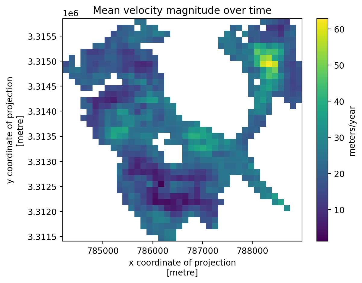
What about Landsat7?
l7_condition = sample_glacier_raster.satellite_img1 == '7'
l7_subset = sample_glacier_raster.sel(mid_date=l7_condition)
l7_subset
<xarray.Dataset> Size: 62MB
Dimensions: (mid_date: 803, y: 37, x: 40)
Coordinates:
* mid_date (mid_date) datetime64[ns] 6kB 2017-11-11T04:1...
* x (x) float64 320B 7.843e+05 ... 7.889e+05
* y (y) float64 296B 3.316e+06 ... 3.311e+06
spatial_ref int64 8B 0
mapping int64 8B 0
Data variables: (12/59)
M11 (mid_date, y, x) float32 5MB nan nan ... nan nan
M11_dr_to_vr_factor (mid_date) float32 3kB nan nan nan ... nan nan
M12 (mid_date, y, x) float32 5MB nan nan ... nan nan
M12_dr_to_vr_factor (mid_date) float32 3kB nan nan nan ... nan nan
acquisition_date_img1 (mid_date) datetime64[ns] 6kB 2017-05-03T04:1...
acquisition_date_img2 (mid_date) datetime64[ns] 6kB 2018-05-22T04:1...
... ...
vy_error_modeled (mid_date) float32 3kB 24.2 24.2 ... 46.5 46.5
vy_error_slow (mid_date) float32 3kB 4.3 5.0 3.4 ... 6.6 9.7
vy_error_stationary (mid_date) float32 3kB 4.3 5.0 3.4 ... 6.6 9.7
vy_stable_shift (mid_date) float32 3kB -0.3 3.2 ... 10.8 3.4
vy_stable_shift_slow (mid_date) float32 3kB -0.3 3.2 ... 10.8 3.4
vy_stable_shift_stationary (mid_date) float32 3kB -0.3 3.2 ... 10.8 3.4
Attributes: (12/19)
Conventions: CF-1.8
GDAL_AREA_OR_POINT: Area
author: ITS_LIVE, a NASA MEaSUREs project (its-live.j...
autoRIFT_parameter_file: http://its-live-data.s3.amazonaws.com/autorif...
datacube_software_version: 1.0
date_created: 25-Sep-2023 22:00:23
... ...
s3: s3://its-live-data/datacubes/v2/N30E090/ITS_L...
skipped_granules: s3://its-live-data/datacubes/v2/N30E090/ITS_L...
time_standard_img1: UTC
time_standard_img2: UTC
title: ITS_LIVE datacube of image pair velocities
url: https://its-live-data.s3.amazonaws.com/datacu...- mid_date: 803
- y: 37
- x: 40
- mid_date(mid_date)datetime64[ns]2017-11-11T04:11:45.280933120 .....
- description :
- midpoint of image 1 and image 2 acquisition date and time with granule's centroid longitude and latitude as microseconds
- standard_name :
- image_pair_center_date_with_time_separation
array(['2017-11-11T04:11:45.280933120', '2017-07-22T04:12:25.815367936', '2017-06-12T04:12:45.944154112', ..., '2017-07-26T04:11:49.029760256', '2017-04-21T04:11:32.560144896', '2018-06-11T04:10:57.953189888'], shape=(803,), dtype='datetime64[ns]') - x(x)float647.843e+05 7.844e+05 ... 7.889e+05
- description :
- x coordinate of projection
- standard_name :
- projection_x_coordinate
- axis :
- X
- long_name :
- x coordinate of projection
- units :
- metre
array([784252.5, 784372.5, 784492.5, 784612.5, 784732.5, 784852.5, 784972.5, 785092.5, 785212.5, 785332.5, 785452.5, 785572.5, 785692.5, 785812.5, 785932.5, 786052.5, 786172.5, 786292.5, 786412.5, 786532.5, 786652.5, 786772.5, 786892.5, 787012.5, 787132.5, 787252.5, 787372.5, 787492.5, 787612.5, 787732.5, 787852.5, 787972.5, 788092.5, 788212.5, 788332.5, 788452.5, 788572.5, 788692.5, 788812.5, 788932.5]) - y(y)float643.316e+06 3.316e+06 ... 3.311e+06
- description :
- y coordinate of projection
- standard_name :
- projection_y_coordinate
- axis :
- Y
- long_name :
- y coordinate of projection
- units :
- metre
array([3315787.5, 3315667.5, 3315547.5, 3315427.5, 3315307.5, 3315187.5, 3315067.5, 3314947.5, 3314827.5, 3314707.5, 3314587.5, 3314467.5, 3314347.5, 3314227.5, 3314107.5, 3313987.5, 3313867.5, 3313747.5, 3313627.5, 3313507.5, 3313387.5, 3313267.5, 3313147.5, 3313027.5, 3312907.5, 3312787.5, 3312667.5, 3312547.5, 3312427.5, 3312307.5, 3312187.5, 3312067.5, 3311947.5, 3311827.5, 3311707.5, 3311587.5, 3311467.5]) - spatial_ref()int640
- GeoTransform :
- 784192.5 120.0 0.0 3315847.5 0.0 -120.0
array(0)
- mapping()int640
- crs_wkt :
- PROJCS["WGS 84 / UTM zone 46N",GEOGCS["WGS 84",DATUM["WGS_1984",SPHEROID["WGS 84",6378137,298.257223563,AUTHORITY["EPSG","7030"]],AUTHORITY["EPSG","6326"]],PRIMEM["Greenwich",0,AUTHORITY["EPSG","8901"]],UNIT["degree",0.0174532925199433,AUTHORITY["EPSG","9122"]],AUTHORITY["EPSG","4326"]],PROJECTION["Transverse_Mercator"],PARAMETER["latitude_of_origin",0],PARAMETER["central_meridian",93],PARAMETER["scale_factor",0.9996],PARAMETER["false_easting",500000],PARAMETER["false_northing",0],UNIT["metre",1,AUTHORITY["EPSG","9001"]],AXIS["Easting",EAST],AXIS["Northing",NORTH],AUTHORITY["EPSG","32646"]]
- semi_major_axis :
- 6378137.0
- semi_minor_axis :
- 6356752.314245179
- inverse_flattening :
- 298.257223563
- reference_ellipsoid_name :
- WGS 84
- longitude_of_prime_meridian :
- 0.0
- prime_meridian_name :
- Greenwich
- geographic_crs_name :
- WGS 84
- horizontal_datum_name :
- World Geodetic System 1984
- projected_crs_name :
- WGS 84 / UTM zone 46N
- grid_mapping_name :
- transverse_mercator
- latitude_of_projection_origin :
- 0.0
- longitude_of_central_meridian :
- 93.0
- false_easting :
- 500000.0
- false_northing :
- 0.0
- scale_factor_at_central_meridian :
- 0.9996
- spatial_ref :
- PROJCS["WGS 84 / UTM zone 46N",GEOGCS["WGS 84",DATUM["WGS_1984",SPHEROID["WGS 84",6378137,298.257223563,AUTHORITY["EPSG","7030"]],AUTHORITY["EPSG","6326"]],PRIMEM["Greenwich",0,AUTHORITY["EPSG","8901"]],UNIT["degree",0.0174532925199433,AUTHORITY["EPSG","9122"]],AUTHORITY["EPSG","4326"]],PROJECTION["Transverse_Mercator"],PARAMETER["latitude_of_origin",0],PARAMETER["central_meridian",93],PARAMETER["scale_factor",0.9996],PARAMETER["false_easting",500000],PARAMETER["false_northing",0],UNIT["metre",1,AUTHORITY["EPSG","9001"]],AXIS["Easting",EAST],AXIS["Northing",NORTH],AUTHORITY["EPSG","32646"]]
- GeoTransform :
- 784192.5 120.0 0.0 3315847.5 0.0 -120.0
array(0)
- M11(mid_date, y, x)float32nan nan nan nan ... nan nan nan nan
- description :
- conversion matrix element (1st row, 1st column) that can be multiplied with vx to give range pixel displacement dr (see Eq. A18 in https://www.mdpi.com/2072-4292/13/4/749)
- standard_name :
- conversion_matrix_element_11
- units :
- pixel/(meter/year)
array([[[nan, nan, nan, ..., nan, nan, nan], [nan, nan, nan, ..., nan, nan, nan], [nan, nan, nan, ..., nan, nan, nan], ..., [nan, nan, nan, ..., nan, nan, nan], [nan, nan, nan, ..., nan, nan, nan], [nan, nan, nan, ..., nan, nan, nan]], [[nan, nan, nan, ..., nan, nan, nan], [nan, nan, nan, ..., nan, nan, nan], [nan, nan, nan, ..., nan, nan, nan], ..., [nan, nan, nan, ..., nan, nan, nan], [nan, nan, nan, ..., nan, nan, nan], [nan, nan, nan, ..., nan, nan, nan]], [[nan, nan, nan, ..., nan, nan, nan], [nan, nan, nan, ..., nan, nan, nan], [nan, nan, nan, ..., nan, nan, nan], ..., ... [nan, nan, nan, ..., nan, nan, nan], [nan, nan, nan, ..., nan, nan, nan], [nan, nan, nan, ..., nan, nan, nan]], [[nan, nan, nan, ..., nan, nan, nan], [nan, nan, nan, ..., nan, nan, nan], [nan, nan, nan, ..., nan, nan, nan], ..., [nan, nan, nan, ..., nan, nan, nan], [nan, nan, nan, ..., nan, nan, nan], [nan, nan, nan, ..., nan, nan, nan]], [[nan, nan, nan, ..., nan, nan, nan], [nan, nan, nan, ..., nan, nan, nan], [nan, nan, nan, ..., nan, nan, nan], ..., [nan, nan, nan, ..., nan, nan, nan], [nan, nan, nan, ..., nan, nan, nan], [nan, nan, nan, ..., nan, nan, nan]]], shape=(803, 37, 40), dtype=float32) - M11_dr_to_vr_factor(mid_date)float32nan nan nan nan ... nan nan nan nan
- description :
- multiplicative factor that converts slant range pixel displacement dr to slant range velocity vr
- standard_name :
- M11_dr_to_vr_factor
- units :
- meter/(year*pixel)
array([nan, nan, nan, nan, nan, nan, nan, nan, nan, nan, nan, nan, nan, nan, nan, nan, nan, nan, nan, nan, nan, nan, nan, nan, nan, nan, nan, nan, nan, nan, nan, nan, nan, nan, nan, nan, nan, nan, nan, nan, nan, nan, nan, nan, nan, nan, nan, nan, nan, nan, nan, nan, nan, nan, nan, nan, nan, nan, nan, nan, nan, nan, nan, nan, nan, nan, nan, nan, nan, nan, nan, nan, nan, nan, nan, nan, nan, nan, nan, nan, nan, nan, nan, nan, nan, nan, nan, nan, nan, nan, nan, nan, nan, nan, nan, nan, nan, nan, nan, nan, nan, nan, nan, nan, nan, nan, nan, nan, nan, nan, nan, nan, nan, nan, nan, nan, nan, nan, nan, nan, nan, nan, nan, nan, nan, nan, nan, nan, nan, nan, nan, nan, nan, nan, nan, nan, nan, nan, nan, nan, nan, nan, nan, nan, nan, nan, nan, nan, nan, nan, nan, nan, nan, nan, nan, nan, nan, nan, nan, nan, nan, nan, nan, nan, nan, nan, nan, nan, nan, nan, nan, nan, nan, nan, nan, nan, nan, nan, nan, nan, nan, nan, nan, nan, nan, nan, nan, nan, nan, nan, nan, nan, nan, nan, nan, nan, nan, nan, nan, nan, nan, nan, nan, nan, nan, nan, nan, nan, nan, nan, nan, nan, nan, nan, nan, nan, nan, nan, nan, nan, nan, nan, nan, nan, nan, nan, nan, nan, nan, nan, nan, nan, nan, nan, nan, nan, nan, nan, nan, nan, nan, nan, nan, nan, nan, nan, nan, nan, nan, nan, nan, nan, nan, nan, nan, nan, nan, nan, nan, nan, ... nan, nan, nan, nan, nan, nan, nan, nan, nan, nan, nan, nan, nan, nan, nan, nan, nan, nan, nan, nan, nan, nan, nan, nan, nan, nan, nan, nan, nan, nan, nan, nan, nan, nan, nan, nan, nan, nan, nan, nan, nan, nan, nan, nan, nan, nan, nan, nan, nan, nan, nan, nan, nan, nan, nan, nan, nan, nan, nan, nan, nan, nan, nan, nan, nan, nan, nan, nan, nan, nan, nan, nan, nan, nan, nan, nan, nan, nan, nan, nan, nan, nan, nan, nan, nan, nan, nan, nan, nan, nan, nan, nan, nan, nan, nan, nan, nan, nan, nan, nan, nan, nan, nan, nan, nan, nan, nan, nan, nan, nan, nan, nan, nan, nan, nan, nan, nan, nan, nan, nan, nan, nan, nan, nan, nan, nan, nan, nan, nan, nan, nan, nan, nan, nan, nan, nan, nan, nan, nan, nan, nan, nan, nan, nan, nan, nan, nan, nan, nan, nan, nan, nan, nan, nan, nan, nan, nan, nan, nan, nan, nan, nan, nan, nan, nan, nan, nan, nan, nan, nan, nan, nan, nan, nan, nan, nan, nan, nan, nan, nan, nan, nan, nan, nan, nan, nan, nan, nan, nan, nan, nan, nan, nan, nan, nan, nan, nan, nan, nan, nan, nan, nan, nan, nan, nan, nan, nan, nan, nan, nan, nan, nan, nan, nan, nan, nan, nan, nan, nan, nan, nan, nan, nan, nan, nan, nan, nan, nan, nan, nan, nan, nan, nan, nan, nan, nan, nan, nan, nan, nan, nan, nan, nan, nan, nan, nan, nan, nan, nan, nan, nan, nan, nan, nan, nan, nan, nan], dtype=float32) - M12(mid_date, y, x)float32nan nan nan nan ... nan nan nan nan
- description :
- conversion matrix element (1st row, 2nd column) that can be multiplied with vy to give range pixel displacement dr (see Eq. A18 in https://www.mdpi.com/2072-4292/13/4/749)
- standard_name :
- conversion_matrix_element_12
- units :
- pixel/(meter/year)
array([[[nan, nan, nan, ..., nan, nan, nan], [nan, nan, nan, ..., nan, nan, nan], [nan, nan, nan, ..., nan, nan, nan], ..., [nan, nan, nan, ..., nan, nan, nan], [nan, nan, nan, ..., nan, nan, nan], [nan, nan, nan, ..., nan, nan, nan]], [[nan, nan, nan, ..., nan, nan, nan], [nan, nan, nan, ..., nan, nan, nan], [nan, nan, nan, ..., nan, nan, nan], ..., [nan, nan, nan, ..., nan, nan, nan], [nan, nan, nan, ..., nan, nan, nan], [nan, nan, nan, ..., nan, nan, nan]], [[nan, nan, nan, ..., nan, nan, nan], [nan, nan, nan, ..., nan, nan, nan], [nan, nan, nan, ..., nan, nan, nan], ..., ... [nan, nan, nan, ..., nan, nan, nan], [nan, nan, nan, ..., nan, nan, nan], [nan, nan, nan, ..., nan, nan, nan]], [[nan, nan, nan, ..., nan, nan, nan], [nan, nan, nan, ..., nan, nan, nan], [nan, nan, nan, ..., nan, nan, nan], ..., [nan, nan, nan, ..., nan, nan, nan], [nan, nan, nan, ..., nan, nan, nan], [nan, nan, nan, ..., nan, nan, nan]], [[nan, nan, nan, ..., nan, nan, nan], [nan, nan, nan, ..., nan, nan, nan], [nan, nan, nan, ..., nan, nan, nan], ..., [nan, nan, nan, ..., nan, nan, nan], [nan, nan, nan, ..., nan, nan, nan], [nan, nan, nan, ..., nan, nan, nan]]], shape=(803, 37, 40), dtype=float32) - M12_dr_to_vr_factor(mid_date)float32nan nan nan nan ... nan nan nan nan
- description :
- multiplicative factor that converts slant range pixel displacement dr to slant range velocity vr
- standard_name :
- M12_dr_to_vr_factor
- units :
- meter/(year*pixel)
array([nan, nan, nan, nan, nan, nan, nan, nan, nan, nan, nan, nan, nan, nan, nan, nan, nan, nan, nan, nan, nan, nan, nan, nan, nan, nan, nan, nan, nan, nan, nan, nan, nan, nan, nan, nan, nan, nan, nan, nan, nan, nan, nan, nan, nan, nan, nan, nan, nan, nan, nan, nan, nan, nan, nan, nan, nan, nan, nan, nan, nan, nan, nan, nan, nan, nan, nan, nan, nan, nan, nan, nan, nan, nan, nan, nan, nan, nan, nan, nan, nan, nan, nan, nan, nan, nan, nan, nan, nan, nan, nan, nan, nan, nan, nan, nan, nan, nan, nan, nan, nan, nan, nan, nan, nan, nan, nan, nan, nan, nan, nan, nan, nan, nan, nan, nan, nan, nan, nan, nan, nan, nan, nan, nan, nan, nan, nan, nan, nan, nan, nan, nan, nan, nan, nan, nan, nan, nan, nan, nan, nan, nan, nan, nan, nan, nan, nan, nan, nan, nan, nan, nan, nan, nan, nan, nan, nan, nan, nan, nan, nan, nan, nan, nan, nan, nan, nan, nan, nan, nan, nan, nan, nan, nan, nan, nan, nan, nan, nan, nan, nan, nan, nan, nan, nan, nan, nan, nan, nan, nan, nan, nan, nan, nan, nan, nan, nan, nan, nan, nan, nan, nan, nan, nan, nan, nan, nan, nan, nan, nan, nan, nan, nan, nan, nan, nan, nan, nan, nan, nan, nan, nan, nan, nan, nan, nan, nan, nan, nan, nan, nan, nan, nan, nan, nan, nan, nan, nan, nan, nan, nan, nan, nan, nan, nan, nan, nan, nan, nan, nan, nan, nan, nan, nan, nan, nan, nan, nan, nan, nan, ... nan, nan, nan, nan, nan, nan, nan, nan, nan, nan, nan, nan, nan, nan, nan, nan, nan, nan, nan, nan, nan, nan, nan, nan, nan, nan, nan, nan, nan, nan, nan, nan, nan, nan, nan, nan, nan, nan, nan, nan, nan, nan, nan, nan, nan, nan, nan, nan, nan, nan, nan, nan, nan, nan, nan, nan, nan, nan, nan, nan, nan, nan, nan, nan, nan, nan, nan, nan, nan, nan, nan, nan, nan, nan, nan, nan, nan, nan, nan, nan, nan, nan, nan, nan, nan, nan, nan, nan, nan, nan, nan, nan, nan, nan, nan, nan, nan, nan, nan, nan, nan, nan, nan, nan, nan, nan, nan, nan, nan, nan, nan, nan, nan, nan, nan, nan, nan, nan, nan, nan, nan, nan, nan, nan, nan, nan, nan, nan, nan, nan, nan, nan, nan, nan, nan, nan, nan, nan, nan, nan, nan, nan, nan, nan, nan, nan, nan, nan, nan, nan, nan, nan, nan, nan, nan, nan, nan, nan, nan, nan, nan, nan, nan, nan, nan, nan, nan, nan, nan, nan, nan, nan, nan, nan, nan, nan, nan, nan, nan, nan, nan, nan, nan, nan, nan, nan, nan, nan, nan, nan, nan, nan, nan, nan, nan, nan, nan, nan, nan, nan, nan, nan, nan, nan, nan, nan, nan, nan, nan, nan, nan, nan, nan, nan, nan, nan, nan, nan, nan, nan, nan, nan, nan, nan, nan, nan, nan, nan, nan, nan, nan, nan, nan, nan, nan, nan, nan, nan, nan, nan, nan, nan, nan, nan, nan, nan, nan, nan, nan, nan, nan, nan, nan, nan, nan, nan, nan], dtype=float32) - acquisition_date_img1(mid_date)datetime64[ns]2017-05-03T04:12:55.171840 ... 2...
- description :
- acquisition date and time of image 1
- standard_name :
- image1_acquition_date
array(['2017-05-03T04:12:55.171840000', '2017-01-11T04:12:39.623214080', '2016-11-08T04:13:04.481691136', '2017-04-01T04:12:42.949755904', '2016-11-24T04:12:59.739601920', '2017-10-26T04:13:06.609417984', '2017-03-16T04:12:38.893263104', '2017-11-27T04:12:59.623030016', '2018-11-30T04:06:36.228204288', '2016-09-21T04:13:12.078295040', '2018-07-25T04:09:25.555763200', '2018-03-03T04:11:49.197383936', '2017-02-12T04:12:23.441945344', '2017-12-29T04:12:40.458198016', '2018-02-15T04:11:59.198033920', '2017-04-01T04:12:42.949755904', '2017-05-03T04:12:55.171840000', '2016-12-10T04:12:56.341405952', '2017-04-01T04:12:42.949755904', '2018-12-16T04:06:10.044793088', '2018-05-22T04:10:35.049019904', '2017-01-27T04:12:29.455911936', '2017-11-11T04:13:04.720666112', '2016-11-24T04:12:59.739601920', '2018-01-14T04:12:27.084400896', '2017-12-13T04:12:51.401551872', '2017-11-11T04:13:04.720666112', '2016-11-08T04:13:04.481691136', '2016-10-23T04:13:11.061116928', '2017-12-29T04:12:40.458198016', '2016-11-24T04:12:59.739601920', '2017-04-01T04:12:42.949755904', '2017-12-29T04:12:40.458198016', '2016-11-08T04:13:04.481691136', '2017-12-13T04:12:51.401551872', '2017-04-01T04:12:42.949755904', '2017-05-03T04:12:55.171840000', '2018-03-03T04:11:49.197383936', '2017-04-01T04:12:42.949755904', '2016-12-10T04:12:56.341405952', ... '2017-04-01T04:12:42.949755904', '2016-10-23T04:13:11.061116928', '2017-03-16T04:12:38.893263104', '2016-08-20T04:13:06.519042048', '2017-01-11T04:12:39.623214080', '2017-01-11T04:12:39.623214080', '2016-08-20T04:13:06.519042048', '2016-08-04T04:13:05.263087872', '2017-04-17T04:12:49.770447872', '2017-03-16T04:12:38.893263104', '2017-06-04T04:13:02.386535936', '2017-05-03T04:12:55.171840000', '2016-08-04T04:13:05.263087872', '2016-08-04T04:13:05.263087872', '2018-07-25T04:09:25.555763200', '2017-04-01T04:12:42.949755904', '2017-05-03T04:12:55.171840000', '2016-10-23T04:13:11.061116928', '2017-05-03T04:12:55.171840000', '2017-04-01T04:12:42.949755904', '2017-06-04T04:13:02.386535936', '2017-06-04T04:13:02.386535936', '2017-02-12T04:12:23.441945344', '2017-04-01T04:12:42.949755904', '2016-09-21T04:13:12.078295040', '2017-01-11T04:12:39.623214080', '2018-07-25T04:09:25.555763200', '2018-03-03T04:11:49.197383936', '2018-07-25T04:09:25.555763200', '2017-03-16T04:12:38.893263104', '2017-04-01T04:12:42.949755904', '2018-03-03T04:11:49.197383936', '2016-10-23T04:13:11.061116928', '2016-10-23T04:13:11.061116928', '2018-07-25T04:09:25.555763200', '2017-06-04T04:13:02.386535936', '2017-06-04T04:13:02.386535936', '2017-01-11T04:12:39.623214080', '2018-03-03T04:11:49.197383936'], dtype='datetime64[ns]') - acquisition_date_img2(mid_date)datetime64[ns]2018-05-22T04:10:35.049019904 .....
- description :
- acquisition date and time of image 2
- standard_name :
- image2_acquition_date
array(['2018-05-22T04:10:35.049019904', '2018-01-30T04:12:11.667300096', '2018-01-14T04:12:27.084400896', '2017-12-29T04:12:40.458198016', '2017-03-16T04:12:38.893263104', '2018-11-30T04:06:36.228204288', '2017-11-11T04:13:04.720666112', '2018-12-16T04:06:10.044793088', '2019-01-01T04:05:41.761686272', '2018-01-14T04:12:27.084400896', '2019-01-01T04:05:41.761686272', '2019-01-17T04:05:11.586401024', '2018-01-14T04:12:27.084400896', '2018-03-03T04:11:49.197383936', '2019-01-17T04:05:11.586401024', '2017-11-27T04:12:59.623030016', '2017-06-04T04:13:02.386535936', '2018-02-15T04:11:59.198033920', '2017-12-13T04:12:51.401551872', '2019-01-17T04:05:11.586401024', '2018-10-29T04:07:21.963168256', '2017-03-16T04:12:38.893263104', '2018-05-22T04:10:35.049019904', '2017-11-11T04:13:04.720666112', '2018-12-16T04:06:10.044793088', '2018-02-15T04:11:59.198033920', '2018-01-14T04:12:27.084400896', '2018-01-30T04:12:11.667300096', '2017-05-03T04:12:55.171840000', '2018-02-15T04:11:59.198033920', '2018-01-30T04:12:11.667300096', '2017-06-04T04:13:02.386535936', '2018-10-29T04:07:21.963168256', '2017-02-28T04:12:32.528041984', '2018-12-16T04:06:10.044793088', '2017-05-03T04:12:55.171840000', '2018-01-30T04:12:11.667300096', '2019-02-18T04:04:12.616978944', '2018-03-03T04:11:49.197383936', '2017-04-01T04:12:42.949755904', ... '2018-03-27T04:09:57.437323008', '2018-03-27T04:09:57.437323008', '2017-07-14T04:10:16.946407936', '2017-09-16T04:10:35.331774976', '2017-04-09T04:09:59.003422976', '2017-09-16T04:10:35.331774976', '2018-02-07T04:10:19.247780096', '2017-07-30T04:10:25.156854016', '2018-02-07T04:10:19.247780096', '2017-04-09T04:09:59.003422976', '2017-12-05T04:10:37.029957888', '2018-02-07T04:10:19.247780096', '2017-12-05T04:10:37.029957888', '2017-09-16T04:10:35.331774976', '2018-12-08T04:10:21.702228992', '2018-09-19T04:10:06.348390144', '2017-07-30T04:10:25.156854016', '2017-07-14T04:10:16.946407936', '2017-09-16T04:10:35.331774976', '2017-04-09T04:09:59.003422976', '2018-04-28T04:09:39.925913088', '2017-07-30T04:10:25.156854016', '2017-07-30T04:10:25.156854016', '2017-07-14T04:10:16.946407936', '2017-07-30T04:10:25.156854016', '2017-07-14T04:10:16.946407936', '2019-01-09T04:10:19.605915904', '2018-03-27T04:09:57.437323008', '2019-01-25T04:10:15.711925760', '2017-07-30T04:10:25.156854016', '2017-07-30T04:10:25.156854016', '2018-05-30T04:09:17.034597888', '2017-07-30T04:10:25.156854016', '2017-04-09T04:09:59.003422976', '2018-12-24T04:10:20.874892032', '2018-02-07T04:10:19.247780096', '2017-09-16T04:10:35.331774976', '2017-07-30T04:10:25.156854016', '2018-09-19T04:10:06.348390144'], dtype='datetime64[ns]') - autoRIFT_software_version(mid_date)object'1.5.0' '1.5.0' ... '1.5.0' '1.5.0'
- description :
- version of autoRIFT software
- standard_name :
- autoRIFT_software_version
array(['1.5.0', '1.5.0', '1.5.0', '1.5.0', '1.5.0', '1.5.0', '1.5.0', '1.5.0', '1.5.0', '1.5.0', '1.5.0', '1.5.0', '1.5.0', '1.5.0', '1.5.0', '1.5.0', '1.5.0', '1.5.0', '1.5.0', '1.5.0', '1.5.0', '1.5.0', '1.5.0', '1.5.0', '1.5.0', '1.5.0', '1.5.0', '1.5.0', '1.5.0', '1.5.0', '1.5.0', '1.5.0', '1.5.0', '1.5.0', '1.5.0', '1.5.0', '1.5.0', '1.5.0', '1.5.0', '1.5.0', '1.5.0', '1.5.0', '1.5.0', '1.5.0', '1.5.0', '1.5.0', '1.5.0', '1.5.0', '1.5.0', '1.5.0', '1.5.0', '1.5.0', '1.5.0', '1.5.0', '1.5.0', '1.5.0', '1.5.0', '1.5.0', '1.5.0', '1.5.0', '1.5.0', '1.5.0', '1.5.0', '1.5.0', '1.5.0', '1.5.0', '1.5.0', '1.5.0', '1.5.0', '1.5.0', '1.5.0', '1.5.0', '1.5.0', '1.5.0', '1.5.0', '1.5.0', '1.5.0', '1.5.0', '1.5.0', '1.5.0', '1.5.0', '1.5.0', '1.5.0', '1.5.0', '1.5.0', '1.5.0', '1.5.0', '1.5.0', '1.5.0', '1.5.0', '1.5.0', '1.5.0', '1.5.0', '1.5.0', '1.5.0', '1.5.0', '1.5.0', '1.5.0', '1.5.0', '1.5.0', '1.5.0', '1.5.0', '1.5.0', '1.5.0', '1.5.0', '1.5.0', '1.5.0', '1.5.0', '1.5.0', '1.5.0', '1.5.0', '1.5.0', '1.5.0', '1.5.0', '1.5.0', '1.5.0', '1.5.0', '1.5.0', '1.5.0', '1.5.0', '1.5.0', '1.5.0', '1.5.0', '1.5.0', '1.5.0', '1.5.0', '1.5.0', '1.5.0', '1.5.0', '1.5.0', '1.5.0', '1.5.0', '1.5.0', '1.5.0', '1.5.0', '1.5.0', '1.5.0', '1.5.0', '1.5.0', '1.5.0', ... '1.5.0', '1.5.0', '1.5.0', '1.5.0', '1.5.0', '1.5.0', '1.5.0', '1.5.0', '1.5.0', '1.5.0', '1.5.0', '1.5.0', '1.5.0', '1.5.0', '1.5.0', '1.5.0', '1.5.0', '1.5.0', '1.5.0', '1.5.0', '1.5.0', '1.5.0', '1.5.0', '1.5.0', '1.5.0', '1.5.0', '1.5.0', '1.5.0', '1.5.0', '1.5.0', '1.5.0', '1.5.0', '1.5.0', '1.5.0', '1.5.0', '1.5.0', '1.5.0', '1.5.0', '1.5.0', '1.5.0', '1.5.0', '1.5.0', '1.5.0', '1.5.0', '1.5.0', '1.5.0', '1.5.0', '1.5.0', '1.5.0', '1.5.0', '1.5.0', '1.5.0', '1.5.0', '1.5.0', '1.5.0', '1.5.0', '1.5.0', '1.5.0', '1.5.0', '1.5.0', '1.5.0', '1.5.0', '1.5.0', '1.5.0', '1.5.0', '1.5.0', '1.5.0', '1.5.0', '1.5.0', '1.5.0', '1.5.0', '1.5.0', '1.5.0', '1.5.0', '1.5.0', '1.5.0', '1.5.0', '1.5.0', '1.5.0', '1.5.0', '1.5.0', '1.5.0', '1.5.0', '1.5.0', '1.5.0', '1.5.0', '1.5.0', '1.5.0', '1.5.0', '1.5.0', '1.5.0', '1.5.0', '1.5.0', '1.5.0', '1.5.0', '1.5.0', '1.5.0', '1.5.0', '1.5.0', '1.5.0', '1.5.0', '1.5.0', '1.5.0', '1.5.0', '1.5.0', '1.5.0', '1.5.0', '1.5.0', '1.5.0', '1.5.0', '1.5.0', '1.5.0', '1.5.0', '1.5.0', '1.5.0', '1.5.0', '1.5.0', '1.5.0', '1.5.0', '1.5.0', '1.5.0', '1.5.0', '1.5.0', '1.5.0', '1.5.0', '1.5.0', '1.5.0', '1.5.0', '1.5.0', '1.5.0', '1.5.0', '1.5.0', '1.5.0', '1.5.0', '1.5.0', '1.5.0', '1.5.0', '1.5.0'], dtype=object) - chip_size_height(mid_date, y, x)float32nan nan nan nan ... nan nan nan nan
- chip_size_coordinates :
- Optical data: chip_size_coordinates = 'image projection geometry: width = x, height = y'. Radar data: chip_size_coordinates = 'radar geometry: width = range, height = azimuth'
- description :
- height of search template (chip)
- standard_name :
- chip_size_height
- units :
- m
- y_pixel_size :
- 10.0
array([[[nan, nan, nan, ..., nan, nan, nan], [nan, nan, nan, ..., nan, nan, nan], [nan, nan, nan, ..., nan, nan, nan], ..., [nan, nan, nan, ..., nan, nan, nan], [nan, nan, nan, ..., nan, nan, nan], [nan, nan, nan, ..., nan, nan, nan]], [[nan, nan, nan, ..., nan, nan, nan], [nan, nan, nan, ..., nan, nan, nan], [nan, nan, nan, ..., nan, nan, nan], ..., [nan, nan, nan, ..., nan, nan, nan], [nan, nan, nan, ..., nan, nan, nan], [nan, nan, nan, ..., nan, nan, nan]], [[nan, nan, nan, ..., nan, nan, nan], [nan, nan, nan, ..., nan, nan, nan], [nan, nan, nan, ..., nan, nan, nan], ..., ... [nan, nan, nan, ..., nan, nan, nan], [nan, nan, nan, ..., nan, nan, nan], [nan, nan, nan, ..., nan, nan, nan]], [[nan, nan, nan, ..., nan, nan, nan], [nan, nan, nan, ..., nan, nan, nan], [nan, nan, nan, ..., nan, nan, nan], ..., [nan, nan, nan, ..., nan, nan, nan], [nan, nan, nan, ..., nan, nan, nan], [nan, nan, nan, ..., nan, nan, nan]], [[nan, nan, nan, ..., nan, nan, nan], [nan, nan, nan, ..., nan, nan, nan], [nan, nan, nan, ..., nan, nan, nan], ..., [nan, nan, nan, ..., nan, nan, nan], [nan, nan, nan, ..., nan, nan, nan], [nan, nan, nan, ..., nan, nan, nan]]], shape=(803, 37, 40), dtype=float32) - chip_size_width(mid_date, y, x)float32nan nan nan nan ... nan nan nan nan
- chip_size_coordinates :
- Optical data: chip_size_coordinates = 'image projection geometry: width = x, height = y'. Radar data: chip_size_coordinates = 'radar geometry: width = range, height = azimuth'
- description :
- width of search template (chip)
- standard_name :
- chip_size_width
- units :
- m
- x_pixel_size :
- 10.0
array([[[nan, nan, nan, ..., nan, nan, nan], [nan, nan, nan, ..., nan, nan, nan], [nan, nan, nan, ..., nan, nan, nan], ..., [nan, nan, nan, ..., nan, nan, nan], [nan, nan, nan, ..., nan, nan, nan], [nan, nan, nan, ..., nan, nan, nan]], [[nan, nan, nan, ..., nan, nan, nan], [nan, nan, nan, ..., nan, nan, nan], [nan, nan, nan, ..., nan, nan, nan], ..., [nan, nan, nan, ..., nan, nan, nan], [nan, nan, nan, ..., nan, nan, nan], [nan, nan, nan, ..., nan, nan, nan]], [[nan, nan, nan, ..., nan, nan, nan], [nan, nan, nan, ..., nan, nan, nan], [nan, nan, nan, ..., nan, nan, nan], ..., ... [nan, nan, nan, ..., nan, nan, nan], [nan, nan, nan, ..., nan, nan, nan], [nan, nan, nan, ..., nan, nan, nan]], [[nan, nan, nan, ..., nan, nan, nan], [nan, nan, nan, ..., nan, nan, nan], [nan, nan, nan, ..., nan, nan, nan], ..., [nan, nan, nan, ..., nan, nan, nan], [nan, nan, nan, ..., nan, nan, nan], [nan, nan, nan, ..., nan, nan, nan]], [[nan, nan, nan, ..., nan, nan, nan], [nan, nan, nan, ..., nan, nan, nan], [nan, nan, nan, ..., nan, nan, nan], ..., [nan, nan, nan, ..., nan, nan, nan], [nan, nan, nan, ..., nan, nan, nan], [nan, nan, nan, ..., nan, nan, nan]]], shape=(803, 37, 40), dtype=float32) - date_center(mid_date)datetime64[ns]2017-11-11T04:11:45.110430208 .....
- description :
- midpoint of image 1 and image 2 acquisition date
- standard_name :
- image_pair_center_date
array(['2017-11-11T04:11:45.110430208', '2017-07-22T04:12:25.645256960', '2017-06-12T04:12:45.783045888', '2017-08-15T04:12:41.703976960', '2017-01-19T04:12:49.316431872', '2018-05-14T04:09:51.418810880', '2017-07-14T04:12:51.806964992', '2018-06-07T04:09:34.833912064', '2018-12-16T04:06:08.994945024', '2017-05-19T04:12:49.581348096', '2018-10-13T04:07:33.658725376', '2018-08-10T04:08:30.391891968', '2017-07-30T04:12:25.263173120', '2018-01-30T04:12:14.827791104', '2018-08-02T04:08:35.392218112', '2017-07-30T04:12:51.286393088', '2017-05-19T04:12:58.779187968', '2017-07-14T04:12:27.769720064', '2017-08-07T04:12:47.175654144', '2019-01-01T04:05:40.815597056', '2018-08-10T04:08:58.506094080', '2017-02-20T04:12:34.174587904', '2018-02-15T04:11:49.884843264', '2017-05-19T04:13:02.230134016', '2018-07-01T04:09:18.564596992', '2018-01-14T04:12:25.299792896', '2017-12-13T04:12:45.902533888', '2017-06-20T04:12:38.074495232', '2017-01-27T04:13:03.116478976', '2018-01-22T04:12:19.828115968', '2017-06-28T04:12:35.703450880', '2017-05-03T04:12:52.668145920', '2018-05-30T04:10:01.210682880', '2017-01-03T04:12:48.504867328', '2018-06-15T04:09:30.723172096', '2017-04-17T04:12:49.060797952', '2017-09-16T04:12:33.419569664', '2018-08-26T04:08:00.907182080', '2017-09-16T04:12:16.073570048', '2017-02-04T04:12:49.645581056', ... '2017-09-28T04:11:20.193539840', '2017-07-10T04:11:34.249220096', '2017-05-15T04:11:27.919834880', '2017-03-04T04:11:50.925408000', '2017-02-24T04:11:19.313317888', '2017-05-15T04:11:37.477494016', '2017-05-15T04:11:42.883410944', '2017-01-31T04:11:45.209970944', '2017-09-12T04:11:34.509114112', '2017-03-28T04:11:18.948343040', '2017-09-04T04:11:49.708247040', '2017-09-20T04:11:37.209809920', '2017-04-05T04:11:51.146522880', '2017-02-24T04:11:50.297432064', '2018-10-01T04:09:53.628996096', '2017-12-25T04:11:24.649072896', '2017-06-16T04:11:40.164346880', '2017-03-04T04:11:44.003762944', '2017-07-10T04:11:45.251808000', '2017-04-05T04:11:20.976590336', '2017-11-15T04:11:21.156224000', '2017-07-02T04:11:43.771695104', '2017-05-07T04:11:24.299398912', '2017-05-23T04:11:29.948081920', '2017-02-24T04:11:48.617574912', '2017-04-13T04:11:28.284811008', '2018-10-17T04:09:52.580839168', '2018-03-15T04:10:53.317353984', '2018-10-25T04:09:50.633844992', '2017-05-23T04:11:32.025059072', '2017-05-31T04:11:34.053305088', '2018-04-16T04:10:33.115990784', '2017-03-12T04:11:48.108985344', '2017-01-15T04:11:35.032270080', '2018-10-09T04:09:53.215326976', '2017-10-06T04:11:40.817157888', '2017-07-26T04:11:48.859155968', '2017-04-21T04:11:32.390033920', '2018-06-11T04:10:57.772887040'], dtype='datetime64[ns]') - date_dt(mid_date)timedelta64[ns]383 days 23:57:40.253906252 ... ...
- description :
- time separation between acquisition of image 1 and image 2
- standard_name :
- image_pair_time_separation
array([33177460253906252, 33177570996093747, 37324763085937495, 23500797363281252, 9676778906250000, 34559609765625000, 20736026367187495, 33177191308593747, 2764745452880856, 41471955175781252, 13823775878906252, 27647601855468747, 29030402636718747, 5529548583984378, 29029991308593747, 20736017138671873, 2764807250976558, 37324741992187495, 22118407910156252, 2764741497802738, 13823807519531252, 4147209558105468, 16588649707031252, 30412805273437495, 29030022949218747, 5529547924804684, 5529562426757810, 38707147265625000, 16588784179687495, 4147158801269531, 37324752539062504, 5529619116210936, 26265280957031252, 9676768359375000, 31794799218750000, 2764812194824216, 23500757812500000, 30412343847656252, 29030347265625000, 9676786816406252, 2764780883789063, 27648021093750000, 44236705078125000, 24883115625000000, 27647649316406252, 31794780761718747, 35942349902343747, 29030009765625000, 11059068164062504, 2764786651611324, 33177570996093747, 5529551879882810, 4147219445800783, 1382373797607423, 29030062500000000, 27647638769531252, 33177565722656252, 29030410546875000, 2764775610351558, 2764771160888675, ... 6220660913085936, 40780657617187495, 22809515625000000, 18662170605468747, 38015796972656252, 25574225976562504, 36633394335937495, 31103775878906252, 4838270800781252, 28339020703125000, 4838440869140621, 43545396972656252, 13132665527343747, 8985432568359378, 29721439160156252, 14515058935546873, 14515072119140621, 29721386425781252, 4838255639648441, 25574312988281252, 31103833886718747, 44927804882812504, 10367858276367189, 33868649707031252, 7603039160156252, 21427076074218747, 46310231250000000, 31103839160156252, 25574249707031252, 2073440148925783, 15897454980468747, 24191844433593747, 42163052343750000, 35251049707031252, 11750456689453126, 46310241796875000, 7603049707031252, 22809425976562504, 11750260253906252, 691036070251464, 28338996972656252, 4838242785644531, 14515081347656252, 8985454321289063, 26956633886718747, 15897457617187495, 14515254052734378, 2073488269042972, 15897650097656252, 11750266845703126, 10367862231445315, 7603047729492189, 24191833886718747, 14515007519531252, 13132855371093747, 21427036523437495, 8985453002929684, 17279865527343747, 17279897167968747], dtype='timedelta64[ns]') - floatingice(y, x, mid_date)float32nan nan nan nan ... nan nan nan nan
- description :
- floating ice mask, 0 = non-floating-ice, 1 = floating-ice
- flag_meanings :
- non-ice ice
- flag_values :
- [0, 1]
- standard_name :
- floating ice mask
- url :
- https://its-live-data.s3.amazonaws.com/autorift_parameters/v001/N46_0120m_floatingice.tif
array([[[nan, nan, nan, ..., nan, nan, nan], [nan, nan, nan, ..., nan, nan, nan], [nan, nan, nan, ..., nan, nan, nan], ..., [ 0., 0., 0., ..., 0., 0., 0.], [nan, nan, nan, ..., nan, nan, nan], [nan, nan, nan, ..., nan, nan, nan]], [[nan, nan, nan, ..., nan, nan, nan], [nan, nan, nan, ..., nan, nan, nan], [nan, nan, nan, ..., nan, nan, nan], ..., [ 0., 0., 0., ..., 0., 0., 0.], [ 0., 0., 0., ..., 0., 0., 0.], [nan, nan, nan, ..., nan, nan, nan]], [[nan, nan, nan, ..., nan, nan, nan], [nan, nan, nan, ..., nan, nan, nan], [nan, nan, nan, ..., nan, nan, nan], ..., ... [nan, nan, nan, ..., nan, nan, nan], [nan, nan, nan, ..., nan, nan, nan], [nan, nan, nan, ..., nan, nan, nan]], [[nan, nan, nan, ..., nan, nan, nan], [nan, nan, nan, ..., nan, nan, nan], [nan, nan, nan, ..., nan, nan, nan], ..., [nan, nan, nan, ..., nan, nan, nan], [nan, nan, nan, ..., nan, nan, nan], [nan, nan, nan, ..., nan, nan, nan]], [[nan, nan, nan, ..., nan, nan, nan], [nan, nan, nan, ..., nan, nan, nan], [nan, nan, nan, ..., nan, nan, nan], ..., [nan, nan, nan, ..., nan, nan, nan], [nan, nan, nan, ..., nan, nan, nan], [nan, nan, nan, ..., nan, nan, nan]]], shape=(37, 40, 803), dtype=float32) - granule_url(mid_date)object'https://its-live-data.s3.amazon...
- description :
- original granule URL
- standard_name :
- granule_url
array(['https://its-live-data.s3.amazonaws.com/velocity_image_pair/landsatOLI/v02/N30E090/LE07_L1TP_135039_20170503_20200831_02_T1_X_LE07_L1TP_135039_20180522_20200829_02_T1_G0120V02_P014.nc', 'https://its-live-data.s3.amazonaws.com/velocity_image_pair/landsatOLI/v02/N30E090/LE07_L1TP_135039_20170111_20200901_02_T1_X_LE07_L1TP_135039_20180130_20200830_02_T1_G0120V02_P016.nc', 'https://its-live-data.s3.amazonaws.com/velocity_image_pair/landsatOLI/v02/N30E090/LE07_L1TP_135039_20161108_20200901_02_T1_X_LE07_L1TP_135039_20180114_20200830_02_T1_G0120V02_P018.nc', 'https://its-live-data.s3.amazonaws.com/velocity_image_pair/landsatOLI/v02/N30E090/LE07_L1TP_135039_20170401_20200831_02_T1_X_LE07_L1TP_135039_20171229_20200830_02_T1_G0120V02_P016.nc', 'https://its-live-data.s3.amazonaws.com/velocity_image_pair/landsatOLI/v02/N30E090/LE07_L1TP_135039_20161124_20200901_02_T1_X_LE07_L1TP_135039_20170316_20200831_02_T1_G0120V02_P026.nc', 'https://its-live-data.s3.amazonaws.com/velocity_image_pair/landsatOLI/v02/N30E090/LE07_L1TP_135039_20171026_20200830_02_T1_X_LE07_L1TP_135039_20181130_20200827_02_T1_G0120V02_P026.nc', 'https://its-live-data.s3.amazonaws.com/velocity_image_pair/landsatOLI/v02/N30E090/LE07_L1TP_135039_20170316_20200831_02_T1_X_LE07_L1TP_135039_20171111_20200830_02_T1_G0120V02_P023.nc', 'https://its-live-data.s3.amazonaws.com/velocity_image_pair/landsatOLI/v02/N30E090/LE07_L1TP_135039_20171127_20200830_02_T1_X_LE07_L1TP_135039_20181216_20200827_02_T1_G0120V02_P062.nc', 'https://its-live-data.s3.amazonaws.com/velocity_image_pair/landsatOLI/v02/N30E090/LE07_L1TP_135039_20181130_20200827_02_T1_X_LE07_L1TP_135039_20190101_20200827_02_T1_G0120V02_P083.nc', 'https://its-live-data.s3.amazonaws.com/velocity_image_pair/landsatOLI/v02/N30E090/LE07_L1TP_135039_20160921_20200902_02_T1_X_LE07_L1TP_135039_20180114_20200830_02_T1_G0120V02_P015.nc', 'https://its-live-data.s3.amazonaws.com/velocity_image_pair/landsatOLI/v02/N30E090/LE07_L1TP_135039_20180725_20200828_02_T1_X_LE07_L1TP_135039_20190101_20200827_02_T1_G0120V02_P013.nc', 'https://its-live-data.s3.amazonaws.com/velocity_image_pair/landsatOLI/v02/N30E090/LE07_L1TP_135039_20180303_20200829_02_T1_X_LE07_L1TP_135039_20190117_20200827_02_T1_G0120V02_P012.nc', 'https://its-live-data.s3.amazonaws.com/velocity_image_pair/landsatOLI/v02/N30E090/LE07_L1TP_135039_20170212_20200901_02_T1_X_LE07_L1TP_135039_20180114_20200830_02_T1_G0120V02_P019.nc', 'https://its-live-data.s3.amazonaws.com/velocity_image_pair/landsatOLI/v02/N30E090/LE07_L1TP_135039_20171229_20200830_02_T1_X_LE07_L1TP_135039_20180303_20200829_02_T1_G0120V02_P006.nc', 'https://its-live-data.s3.amazonaws.com/velocity_image_pair/landsatOLI/v02/N30E090/LE07_L1TP_135039_20180215_20200829_02_T1_X_LE07_L1TP_135039_20190117_20200827_02_T1_G0120V02_P069.nc', 'https://its-live-data.s3.amazonaws.com/velocity_image_pair/landsatOLI/v02/N30E090/LE07_L1TP_135039_20170401_20200831_02_T1_X_LE07_L1TP_135039_20171127_20200830_02_T1_G0120V02_P016.nc', 'https://its-live-data.s3.amazonaws.com/velocity_image_pair/landsatOLI/v02/N30E090/LE07_L1TP_135039_20170503_20200831_02_T1_X_LE07_L1TP_135039_20170604_20200831_02_T1_G0120V02_P021.nc', 'https://its-live-data.s3.amazonaws.com/velocity_image_pair/landsatOLI/v02/N30E090/LE07_L1TP_135039_20161210_20201008_02_T1_X_LE07_L1TP_135039_20180215_20200829_02_T1_G0120V02_P076.nc', 'https://its-live-data.s3.amazonaws.com/velocity_image_pair/landsatOLI/v02/N30E090/LE07_L1TP_135039_20170401_20200831_02_T1_X_LE07_L1TP_135039_20171213_20200830_02_T1_G0120V02_P019.nc', 'https://its-live-data.s3.amazonaws.com/velocity_image_pair/landsatOLI/v02/N30E090/LE07_L1TP_135039_20181216_20200827_02_T1_X_LE07_L1TP_135039_20190117_20200827_02_T1_G0120V02_P089.nc', ... 'https://its-live-data.s3.amazonaws.com/velocity_image_pair/landsatOLI/v02/N30E090/LE07_L1TP_135039_20170604_20200831_02_T1_X_LC08_L1TP_135039_20180428_20200901_02_T1_G0120V02_P008.nc', 'https://its-live-data.s3.amazonaws.com/velocity_image_pair/landsatOLI/v02/N30E090/LE07_L1TP_135039_20170604_20200831_02_T1_X_LC08_L1TP_135039_20170730_20200903_02_T1_G0120V02_P008.nc', 'https://its-live-data.s3.amazonaws.com/velocity_image_pair/landsatOLI/v02/N30E090/LE07_L1TP_135039_20170212_20200901_02_T1_X_LC08_L1TP_135039_20170730_20200903_02_T1_G0120V02_P009.nc', 'https://its-live-data.s3.amazonaws.com/velocity_image_pair/landsatOLI/v02/N30E090/LE07_L1TP_135039_20170401_20200831_02_T1_X_LC08_L1TP_135039_20170714_20200903_02_T1_G0120V02_P009.nc', 'https://its-live-data.s3.amazonaws.com/velocity_image_pair/landsatOLI/v02/N30E090/LE07_L1TP_135039_20160921_20200902_02_T1_X_LC08_L1TP_135039_20170730_20200903_02_T1_G0120V02_P008.nc', 'https://its-live-data.s3.amazonaws.com/velocity_image_pair/landsatOLI/v02/N30E090/LE07_L1TP_135039_20170111_20200901_02_T1_X_LC08_L1TP_135039_20170714_20200903_02_T1_G0120V02_P007.nc', 'https://its-live-data.s3.amazonaws.com/velocity_image_pair/landsatOLI/v02/N30E090/LE07_L1TP_135039_20180725_20200828_02_T1_X_LC08_L1TP_135039_20190109_20200829_02_T1_G0120V02_P007.nc', 'https://its-live-data.s3.amazonaws.com/velocity_image_pair/landsatOLI/v02/N30E090/LE07_L1TP_135039_20180303_20200829_02_T1_X_LC08_L1TP_135039_20180327_20200901_02_T1_G0120V02_P007.nc', 'https://its-live-data.s3.amazonaws.com/velocity_image_pair/landsatOLI/v02/N30E090/LE07_L1TP_135039_20180725_20200828_02_T1_X_LC08_L1TP_135039_20190125_20200830_02_T1_G0120V02_P007.nc', 'https://its-live-data.s3.amazonaws.com/velocity_image_pair/landsatOLI/v02/N30E090/LE07_L1TP_135039_20170316_20200831_02_T1_X_LC08_L1TP_135039_20170730_20200903_02_T1_G0120V02_P006.nc', 'https://its-live-data.s3.amazonaws.com/velocity_image_pair/landsatOLI/v02/N30E090/LE07_L1TP_135039_20170401_20200831_02_T1_X_LC08_L1TP_135039_20170730_20200903_02_T1_G0120V02_P006.nc', 'https://its-live-data.s3.amazonaws.com/velocity_image_pair/landsatOLI/v02/N30E090/LE07_L1TP_135039_20180303_20200829_02_T1_X_LC08_L1TP_135039_20180530_20200831_02_T1_G0120V02_P007.nc', 'https://its-live-data.s3.amazonaws.com/velocity_image_pair/landsatOLI/v02/N30E090/LE07_L1TP_135039_20161023_20200901_02_T1_X_LC08_L1TP_135039_20170730_20200903_02_T1_G0120V02_P007.nc', 'https://its-live-data.s3.amazonaws.com/velocity_image_pair/landsatOLI/v02/N30E090/LE07_L1TP_135039_20161023_20200901_02_T1_X_LC08_L1TP_135039_20170409_20200904_02_T1_G0120V02_P007.nc', 'https://its-live-data.s3.amazonaws.com/velocity_image_pair/landsatOLI/v02/N30E090/LE07_L1TP_135039_20180725_20200828_02_T1_X_LC08_L1TP_135039_20181224_20200830_02_T1_G0120V02_P006.nc', 'https://its-live-data.s3.amazonaws.com/velocity_image_pair/landsatOLI/v02/N30E090/LE07_L1TP_135039_20170604_20200831_02_T1_X_LC08_L1TP_135039_20180207_20200902_02_T1_G0120V02_P005.nc', 'https://its-live-data.s3.amazonaws.com/velocity_image_pair/landsatOLI/v02/N30E090/LE07_L1TP_135039_20170604_20200831_02_T1_X_LC08_L1TP_135039_20170916_20200903_02_T1_G0120V02_P004.nc', 'https://its-live-data.s3.amazonaws.com/velocity_image_pair/landsatOLI/v02/N30E090/LE07_L1TP_135039_20170111_20200901_02_T1_X_LC08_L1TP_135039_20170730_20200903_02_T1_G0120V02_P004.nc', 'https://its-live-data.s3.amazonaws.com/velocity_image_pair/landsatOLI/v02/N30E090/LE07_L1TP_135039_20180303_20200829_02_T1_X_LC08_L1TP_135039_20180919_20200830_02_T1_G0120V02_P004.nc'], dtype=object) - interp_mask(mid_date, y, x)float32nan nan nan nan ... nan nan nan nan
- description :
- light interpolation mask
- flag_meanings :
- measured interpolated
- flag_values :
- [0, 1]
- standard_name :
- interpolated_value_mask
array([[[nan, nan, nan, ..., nan, nan, nan], [nan, nan, nan, ..., nan, nan, nan], [nan, nan, nan, ..., nan, nan, nan], ..., [nan, nan, nan, ..., nan, nan, nan], [nan, nan, nan, ..., nan, nan, nan], [nan, nan, nan, ..., nan, nan, nan]], [[nan, nan, nan, ..., nan, nan, nan], [nan, nan, nan, ..., nan, nan, nan], [nan, nan, nan, ..., nan, nan, nan], ..., [nan, nan, nan, ..., nan, nan, nan], [nan, nan, nan, ..., nan, nan, nan], [nan, nan, nan, ..., nan, nan, nan]], [[nan, nan, nan, ..., nan, nan, nan], [nan, nan, nan, ..., nan, nan, nan], [nan, nan, nan, ..., nan, nan, nan], ..., ... [nan, nan, nan, ..., nan, nan, nan], [nan, nan, nan, ..., nan, nan, nan], [nan, nan, nan, ..., nan, nan, nan]], [[nan, nan, nan, ..., nan, nan, nan], [nan, nan, nan, ..., nan, nan, nan], [nan, nan, nan, ..., nan, nan, nan], ..., [nan, nan, nan, ..., nan, nan, nan], [nan, nan, nan, ..., nan, nan, nan], [nan, nan, nan, ..., nan, nan, nan]], [[nan, nan, nan, ..., nan, nan, nan], [nan, nan, nan, ..., nan, nan, nan], [nan, nan, nan, ..., nan, nan, nan], ..., [nan, nan, nan, ..., nan, nan, nan], [nan, nan, nan, ..., nan, nan, nan], [nan, nan, nan, ..., nan, nan, nan]]], shape=(803, 37, 40), dtype=float32) - landice(y, x, mid_date)float32nan nan nan nan ... nan nan nan nan
- description :
- land ice mask, 0 = non-land-ice, 1 = land-ice
- flag_meanings :
- non-ice ice
- flag_values :
- [0, 1]
- standard_name :
- land ice mask
- url :
- https://its-live-data.s3.amazonaws.com/autorift_parameters/v001/N46_0120m_landice.tif
array([[[nan, nan, nan, ..., nan, nan, nan], [nan, nan, nan, ..., nan, nan, nan], [nan, nan, nan, ..., nan, nan, nan], ..., [ 1., 1., 1., ..., 1., 1., 1.], [nan, nan, nan, ..., nan, nan, nan], [nan, nan, nan, ..., nan, nan, nan]], [[nan, nan, nan, ..., nan, nan, nan], [nan, nan, nan, ..., nan, nan, nan], [nan, nan, nan, ..., nan, nan, nan], ..., [ 1., 1., 1., ..., 1., 1., 1.], [ 1., 1., 1., ..., 1., 1., 1.], [nan, nan, nan, ..., nan, nan, nan]], [[nan, nan, nan, ..., nan, nan, nan], [nan, nan, nan, ..., nan, nan, nan], [nan, nan, nan, ..., nan, nan, nan], ..., ... [nan, nan, nan, ..., nan, nan, nan], [nan, nan, nan, ..., nan, nan, nan], [nan, nan, nan, ..., nan, nan, nan]], [[nan, nan, nan, ..., nan, nan, nan], [nan, nan, nan, ..., nan, nan, nan], [nan, nan, nan, ..., nan, nan, nan], ..., [nan, nan, nan, ..., nan, nan, nan], [nan, nan, nan, ..., nan, nan, nan], [nan, nan, nan, ..., nan, nan, nan]], [[nan, nan, nan, ..., nan, nan, nan], [nan, nan, nan, ..., nan, nan, nan], [nan, nan, nan, ..., nan, nan, nan], ..., [nan, nan, nan, ..., nan, nan, nan], [nan, nan, nan, ..., nan, nan, nan], [nan, nan, nan, ..., nan, nan, nan]]], shape=(37, 40, 803), dtype=float32) - mission_img1(mid_date)object'L' 'L' 'L' 'L' ... 'L' 'L' 'L' 'L'
- description :
- id of the mission that acquired image 1
- standard_name :
- image1_mission
array(['L', 'L', 'L', 'L', 'L', 'L', 'L', 'L', 'L', 'L', 'L', 'L', 'L', 'L', 'L', 'L', 'L', 'L', 'L', 'L', 'L', 'L', 'L', 'L', 'L', 'L', 'L', 'L', 'L', 'L', 'L', 'L', 'L', 'L', 'L', 'L', 'L', 'L', 'L', 'L', 'L', 'L', 'L', 'L', 'L', 'L', 'L', 'L', 'L', 'L', 'L', 'L', 'L', 'L', 'L', 'L', 'L', 'L', 'L', 'L', 'L', 'L', 'L', 'L', 'L', 'L', 'L', 'L', 'L', 'L', 'L', 'L', 'L', 'L', 'L', 'L', 'L', 'L', 'L', 'L', 'L', 'L', 'L', 'L', 'L', 'L', 'L', 'L', 'L', 'L', 'L', 'L', 'L', 'L', 'L', 'L', 'L', 'L', 'L', 'L', 'L', 'L', 'L', 'L', 'L', 'L', 'L', 'L', 'L', 'L', 'L', 'L', 'L', 'L', 'L', 'L', 'L', 'L', 'L', 'L', 'L', 'L', 'L', 'L', 'L', 'L', 'L', 'L', 'L', 'L', 'L', 'L', 'L', 'L', 'L', 'L', 'L', 'L', 'L', 'L', 'L', 'L', 'L', 'L', 'L', 'L', 'L', 'L', 'L', 'L', 'L', 'L', 'L', 'L', 'L', 'L', 'L', 'L', 'L', 'L', 'L', 'L', 'L', 'L', 'L', 'L', 'L', 'L', 'L', 'L', 'L', 'L', 'L', 'L', 'L', 'L', 'L', 'L', 'L', 'L', 'L', 'L', 'L', 'L', 'L', 'L', 'L', 'L', 'L', 'L', 'L', 'L', 'L', 'L', 'L', 'L', 'L', 'L', 'L', 'L', 'L', 'L', 'L', 'L', 'L', 'L', 'L', 'L', 'L', 'L', 'L', 'L', 'L', 'L', 'L', 'L', 'L', 'L', 'L', 'L', 'L', 'L', 'L', 'L', 'L', 'L', 'L', 'L', 'L', 'L', 'L', 'L', 'L', 'L', 'L', 'L', 'L', 'L', 'L', 'L', 'L', 'L', 'L', 'L', 'L', 'L', 'L', 'L', 'L', 'L', 'L', 'L', 'L', 'L', 'L', 'L', 'L', 'L', 'L', 'L', ... 'L', 'L', 'L', 'L', 'L', 'L', 'L', 'L', 'L', 'L', 'L', 'L', 'L', 'L', 'L', 'L', 'L', 'L', 'L', 'L', 'L', 'L', 'L', 'L', 'L', 'L', 'L', 'L', 'L', 'L', 'L', 'L', 'L', 'L', 'L', 'L', 'L', 'L', 'L', 'L', 'L', 'L', 'L', 'L', 'L', 'L', 'L', 'L', 'L', 'L', 'L', 'L', 'L', 'L', 'L', 'L', 'L', 'L', 'L', 'L', 'L', 'L', 'L', 'L', 'L', 'L', 'L', 'L', 'L', 'L', 'L', 'L', 'L', 'L', 'L', 'L', 'L', 'L', 'L', 'L', 'L', 'L', 'L', 'L', 'L', 'L', 'L', 'L', 'L', 'L', 'L', 'L', 'L', 'L', 'L', 'L', 'L', 'L', 'L', 'L', 'L', 'L', 'L', 'L', 'L', 'L', 'L', 'L', 'L', 'L', 'L', 'L', 'L', 'L', 'L', 'L', 'L', 'L', 'L', 'L', 'L', 'L', 'L', 'L', 'L', 'L', 'L', 'L', 'L', 'L', 'L', 'L', 'L', 'L', 'L', 'L', 'L', 'L', 'L', 'L', 'L', 'L', 'L', 'L', 'L', 'L', 'L', 'L', 'L', 'L', 'L', 'L', 'L', 'L', 'L', 'L', 'L', 'L', 'L', 'L', 'L', 'L', 'L', 'L', 'L', 'L', 'L', 'L', 'L', 'L', 'L', 'L', 'L', 'L', 'L', 'L', 'L', 'L', 'L', 'L', 'L', 'L', 'L', 'L', 'L', 'L', 'L', 'L', 'L', 'L', 'L', 'L', 'L', 'L', 'L', 'L', 'L', 'L', 'L', 'L', 'L', 'L', 'L', 'L', 'L', 'L', 'L', 'L', 'L', 'L', 'L', 'L', 'L', 'L', 'L', 'L', 'L', 'L', 'L', 'L', 'L', 'L', 'L', 'L', 'L', 'L', 'L', 'L', 'L', 'L', 'L', 'L', 'L', 'L', 'L', 'L', 'L', 'L', 'L', 'L', 'L', 'L', 'L', 'L', 'L', 'L', 'L', 'L', 'L', 'L', 'L', 'L', 'L', 'L', 'L', 'L', 'L'], dtype=object) - mission_img2(mid_date)object'L' 'L' 'L' 'L' ... 'L' 'L' 'L' 'L'
- description :
- id of the mission that acquired image 2
- standard_name :
- image2_mission
array(['L', 'L', 'L', 'L', 'L', 'L', 'L', 'L', 'L', 'L', 'L', 'L', 'L', 'L', 'L', 'L', 'L', 'L', 'L', 'L', 'L', 'L', 'L', 'L', 'L', 'L', 'L', 'L', 'L', 'L', 'L', 'L', 'L', 'L', 'L', 'L', 'L', 'L', 'L', 'L', 'L', 'L', 'L', 'L', 'L', 'L', 'L', 'L', 'L', 'L', 'L', 'L', 'L', 'L', 'L', 'L', 'L', 'L', 'L', 'L', 'L', 'L', 'L', 'L', 'L', 'L', 'L', 'L', 'L', 'L', 'L', 'L', 'L', 'L', 'L', 'L', 'L', 'L', 'L', 'L', 'L', 'L', 'L', 'L', 'L', 'L', 'L', 'L', 'L', 'L', 'L', 'L', 'L', 'L', 'L', 'L', 'L', 'L', 'L', 'L', 'L', 'L', 'L', 'L', 'L', 'L', 'L', 'L', 'L', 'L', 'L', 'L', 'L', 'L', 'L', 'L', 'L', 'L', 'L', 'L', 'L', 'L', 'L', 'L', 'L', 'L', 'L', 'L', 'L', 'L', 'L', 'L', 'L', 'L', 'L', 'L', 'L', 'L', 'L', 'L', 'L', 'L', 'L', 'L', 'L', 'L', 'L', 'L', 'L', 'L', 'L', 'L', 'L', 'L', 'L', 'L', 'L', 'L', 'L', 'L', 'L', 'L', 'L', 'L', 'L', 'L', 'L', 'L', 'L', 'L', 'L', 'L', 'L', 'L', 'L', 'L', 'L', 'L', 'L', 'L', 'L', 'L', 'L', 'L', 'L', 'L', 'L', 'L', 'L', 'L', 'L', 'L', 'L', 'L', 'L', 'L', 'L', 'L', 'L', 'L', 'L', 'L', 'L', 'L', 'L', 'L', 'L', 'L', 'L', 'L', 'L', 'L', 'L', 'L', 'L', 'L', 'L', 'L', 'L', 'L', 'L', 'L', 'L', 'L', 'L', 'L', 'L', 'L', 'L', 'L', 'L', 'L', 'L', 'L', 'L', 'L', 'L', 'L', 'L', 'L', 'L', 'L', 'L', 'L', 'L', 'L', 'L', 'L', 'L', 'L', 'L', 'L', 'L', 'L', 'L', 'L', 'L', 'L', 'L', 'L', ... 'L', 'L', 'L', 'L', 'L', 'L', 'L', 'L', 'L', 'L', 'L', 'L', 'L', 'L', 'L', 'L', 'L', 'L', 'L', 'L', 'L', 'L', 'L', 'L', 'L', 'L', 'L', 'L', 'L', 'L', 'L', 'L', 'L', 'L', 'L', 'L', 'L', 'L', 'L', 'L', 'L', 'L', 'L', 'L', 'L', 'L', 'L', 'L', 'L', 'L', 'L', 'L', 'L', 'L', 'L', 'L', 'L', 'L', 'L', 'L', 'L', 'L', 'L', 'L', 'L', 'L', 'L', 'L', 'L', 'L', 'L', 'L', 'L', 'L', 'L', 'L', 'L', 'L', 'L', 'L', 'L', 'L', 'L', 'L', 'L', 'L', 'L', 'L', 'L', 'L', 'L', 'L', 'L', 'L', 'L', 'L', 'L', 'L', 'L', 'L', 'L', 'L', 'L', 'L', 'L', 'L', 'L', 'L', 'L', 'L', 'L', 'L', 'L', 'L', 'L', 'L', 'L', 'L', 'L', 'L', 'L', 'L', 'L', 'L', 'L', 'L', 'L', 'L', 'L', 'L', 'L', 'L', 'L', 'L', 'L', 'L', 'L', 'L', 'L', 'L', 'L', 'L', 'L', 'L', 'L', 'L', 'L', 'L', 'L', 'L', 'L', 'L', 'L', 'L', 'L', 'L', 'L', 'L', 'L', 'L', 'L', 'L', 'L', 'L', 'L', 'L', 'L', 'L', 'L', 'L', 'L', 'L', 'L', 'L', 'L', 'L', 'L', 'L', 'L', 'L', 'L', 'L', 'L', 'L', 'L', 'L', 'L', 'L', 'L', 'L', 'L', 'L', 'L', 'L', 'L', 'L', 'L', 'L', 'L', 'L', 'L', 'L', 'L', 'L', 'L', 'L', 'L', 'L', 'L', 'L', 'L', 'L', 'L', 'L', 'L', 'L', 'L', 'L', 'L', 'L', 'L', 'L', 'L', 'L', 'L', 'L', 'L', 'L', 'L', 'L', 'L', 'L', 'L', 'L', 'L', 'L', 'L', 'L', 'L', 'L', 'L', 'L', 'L', 'L', 'L', 'L', 'L', 'L', 'L', 'L', 'L', 'L', 'L', 'L', 'L', 'L', 'L'], dtype=object) - roi_valid_percentage(mid_date)float3214.0 16.9 18.0 16.0 ... 4.2 4.2 4.0
- description :
- percentage of pixels with a valid velocity estimate determined for the intersection of the full image pair footprint and the region of interest (roi) that defines where autoRIFT tried to estimate a velocity
- standard_name :
- region_of_interest_valid_pixel_percentage
array([14. , 16.9, 18. , 16. , 26.8, 26.2, 23.9, 62.3, 83. , 15. , 13.8, 12.7, 19. , 6.2, 69.6, 16.3, 21.3, 76.8, 19. , 89. , 3.4, 28.4, 23.9, 83. , 24.7, 49.4, 33. , 44. , 11.9, 66. , 53.2, 5.5, 37.9, 60.7, 54.6, 16. , 12.6, 6.6, 10. , 19.6, 54.9, 72. , 15.8, 24.9, 13.1, 76.8, 5.7, 56.7, 15.1, 67.2, 81.2, 19.9, 19. , 72. , 31.6, 58.8, 8.9, 24.6, 31. , 58. , 16.7, 17.6, 26.7, 31.1, 28.6, 88. , 69. , 12. , 21.7, 37.4, 21.9, 46.8, 20.7, 20.4, 48.5, 19.7, 23.5, 29.9, 7.8, 36.7, 31.7, 63.7, 25.7, 10. , 7.5, 25. , 20.5, 6.4, 20.5, 3.7, 13.6, 39.3, 26.3, 43.3, 20.5, 27.7, 8.5, 17.2, 10.3, 7.1, 19.8, 27.8, 44.5, 15.8, 46.7, 37.8, 7.2, 39.1, 55.9, 88. , 32. , 56.4, 33.9, 24.6, 17.5, 54. , 24.9, 28.4, 15. , 47.6, 29.4, 11.2, 36.7, 23.5, 11.5, 5.6, 9.2, 23.3, 18.9, 22.8, 58.9, 4.5, 51.9, 31. , 45.3, 19.9, 43.8, 16.8, 39.1, 25.4, 65.9, 44.6, 23.9, 18. , 8.6, 68.7, 17. , 25.5, 63.9, 20.3, 21.7, 31.9, 24.1, 7.1, 15.3, 5.6, 18.1, 62.9, 11. , 27.6, 18.3, 68.5, 26.3, 50. , 25.3, 5. , 18.9, 29.6, 15.1, 4.3, 48.6, 5.5, 72.6, 63. , 50.2, 46.2, 21. , 36.8, 13.4, 53. , 51.5, 34.7, 25. , 15.3, 3.5, 41.7, 34.1, 7.1, 74.2, 10.9, 3.2, 25.2, 18.1, 17.7, 19.7, 58. , 26.8, 12.7, 53. , 22.6, 8. , 62. , 20.4, 27.6, 80. , 11.2, 9.4, 8. , 47.1, 10.9, 11. , 15. , 19. , 51.9, 23.3, 33.8, 55.4, 17.3, 13.2, 32. , ... 29.9, 30.2, 29.1, 28.8, 28.6, 28.5, 28.9, 29.3, 29.2, 28.5, 28.9, 29.2, 28.6, 29.1, 28.8, 29.3, 27.8, 27.5, 28. , 27.6, 28.2, 28.4, 28.3, 27.6, 27.3, 27.1, 27.3, 26.9, 27.4, 26.8, 27. , 26. , 26.3, 26. , 26. , 26.1, 26.2, 26.4, 26.2, 26.1, 25.8, 26. , 25.8, 26.4, 25. , 25.3, 24.8, 25. , 24.6, 24.7, 24.9, 25. , 25.1, 23.8, 23.9, 24.2, 23.8, 23.6, 24.2, 23.9, 23.6, 24.4, 23.7, 23.8, 23.3, 23.3, 23.4, 23.1, 23.3, 22.7, 22.7, 23.1, 21.6, 22.3, 21.9, 21.5, 22. , 21.9, 21.7, 21.6, 22. , 22. , 21. , 21. , 21.3, 21.2, 21. , 20.8, 21. , 20.9, 20.7, 20.7, 21. , 20.7, 19.5, 19.9, 20.2, 19.9, 20.3, 19.9, 18.9, 19.3, 18.9, 18.9, 19.4, 19. , 19.4, 19.1, 18.7, 19. , 18.4, 18. , 18.2, 17.7, 18. , 17.8, 17.8, 17.9, 17.5, 18.1, 18. , 17.6, 18. , 18.1, 17.3, 17.3, 16.5, 17. , 17.4, 16.8, 16.7, 17.4, 17.1, 16.7, 16.2, 16.1, 15.7, 15.5, 16.3, 16. , 16.4, 16.2, 15.4, 15. , 14.9, 15.1, 14.8, 14.8, 15. , 14.6, 15.4, 14.8, 15.4, 14.1, 14.4, 14.4, 14.3, 14.3, 13.1, 13.4, 12.5, 12.9, 12.9, 12.8, 13.2, 13.1, 13. , 13.3, 11.6, 11.8, 11.9, 11.7, 11.6, 12.4, 11.6, 11.9, 11.6, 11.7, 12. , 12. , 10.5, 11.2, 11.2, 10.8, 9.7, 10.3, 10. , 9.7, 9.7, 9.5, 8.6, 8.5, 9.1, 9.1, 8.3, 7.7, 7.9, 7.6, 7.8, 6.7, 6.6, 7. , 7.1, 7.3, 6.8, 5.3, 4.2, 4.2, 4. ], dtype=float32) - satellite_img1(mid_date)object'7' '7' '7' '7' ... '7' '7' '7' '7'
- description :
- id of the satellite that acquired image 1
- standard_name :
- image1_satellite
array(['7', '7', '7', '7', '7', '7', '7', '7', '7', '7', '7', '7', '7', '7', '7', '7', '7', '7', '7', '7', '7', '7', '7', '7', '7', '7', '7', '7', '7', '7', '7', '7', '7', '7', '7', '7', '7', '7', '7', '7', '7', '7', '7', '7', '7', '7', '7', '7', '7', '7', '7', '7', '7', '7', '7', '7', '7', '7', '7', '7', '7', '7', '7', '7', '7', '7', '7', '7', '7', '7', '7', '7', '7', '7', '7', '7', '7', '7', '7', '7', '7', '7', '7', '7', '7', '7', '7', '7', '7', '7', '7', '7', '7', '7', '7', '7', '7', '7', '7', '7', '7', '7', '7', '7', '7', '7', '7', '7', '7', '7', '7', '7', '7', '7', '7', '7', '7', '7', '7', '7', '7', '7', '7', '7', '7', '7', '7', '7', '7', '7', '7', '7', '7', '7', '7', '7', '7', '7', '7', '7', '7', '7', '7', '7', '7', '7', '7', '7', '7', '7', '7', '7', '7', '7', '7', '7', '7', '7', '7', '7', '7', '7', '7', '7', '7', '7', '7', '7', '7', '7', '7', '7', '7', '7', '7', '7', '7', '7', '7', '7', '7', '7', '7', '7', '7', '7', '7', '7', '7', '7', '7', '7', '7', '7', '7', '7', '7', '7', '7', '7', '7', '7', '7', '7', '7', '7', '7', '7', '7', '7', '7', '7', '7', '7', '7', '7', '7', '7', '7', '7', '7', '7', '7', '7', '7', '7', '7', '7', '7', '7', '7', '7', '7', '7', '7', '7', '7', '7', '7', '7', '7', '7', '7', '7', '7', '7', '7', '7', '7', '7', '7', '7', '7', '7', '7', '7', '7', '7', '7', '7', ... '7', '7', '7', '7', '7', '7', '7', '7', '7', '7', '7', '7', '7', '7', '7', '7', '7', '7', '7', '7', '7', '7', '7', '7', '7', '7', '7', '7', '7', '7', '7', '7', '7', '7', '7', '7', '7', '7', '7', '7', '7', '7', '7', '7', '7', '7', '7', '7', '7', '7', '7', '7', '7', '7', '7', '7', '7', '7', '7', '7', '7', '7', '7', '7', '7', '7', '7', '7', '7', '7', '7', '7', '7', '7', '7', '7', '7', '7', '7', '7', '7', '7', '7', '7', '7', '7', '7', '7', '7', '7', '7', '7', '7', '7', '7', '7', '7', '7', '7', '7', '7', '7', '7', '7', '7', '7', '7', '7', '7', '7', '7', '7', '7', '7', '7', '7', '7', '7', '7', '7', '7', '7', '7', '7', '7', '7', '7', '7', '7', '7', '7', '7', '7', '7', '7', '7', '7', '7', '7', '7', '7', '7', '7', '7', '7', '7', '7', '7', '7', '7', '7', '7', '7', '7', '7', '7', '7', '7', '7', '7', '7', '7', '7', '7', '7', '7', '7', '7', '7', '7', '7', '7', '7', '7', '7', '7', '7', '7', '7', '7', '7', '7', '7', '7', '7', '7', '7', '7', '7', '7', '7', '7', '7', '7', '7', '7', '7', '7', '7', '7', '7', '7', '7', '7', '7', '7', '7', '7', '7', '7', '7', '7', '7', '7', '7', '7', '7', '7', '7', '7', '7', '7', '7', '7', '7', '7', '7', '7', '7', '7', '7', '7', '7', '7', '7', '7', '7', '7', '7', '7', '7', '7', '7', '7', '7', '7', '7', '7', '7', '7', '7', '7', '7', '7', '7', '7', '7'], dtype=object) - satellite_img2(mid_date)object'7' '7' '7' '7' ... '8' '8' '8' '8'
- description :
- id of the satellite that acquired image 2
- standard_name :
- image2_satellite
array(['7', '7', '7', '7', '7', '7', '7', '7', '7', '7', '7', '7', '7', '7', '7', '7', '7', '7', '7', '7', '7', '7', '7', '7', '7', '7', '7', '7', '7', '7', '7', '7', '7', '7', '7', '7', '7', '7', '7', '7', '7', '7', '7', '7', '7', '7', '7', '7', '7', '7', '7', '7', '7', '7', '7', '7', '7', '7', '7', '7', '7', '7', '7', '7', '7', '7', '7', '7', '7', '7', '7', '7', '7', '7', '7', '7', '7', '7', '7', '7', '7', '7', '7', '7', '7', '7', '7', '7', '7', '7', '7', '7', '7', '7', '7', '7', '7', '7', '7', '7', '7', '7', '7', '7', '7', '7', '7', '7', '7', '7', '7', '7', '7', '7', '7', '7', '7', '7', '7', '7', '7', '7', '7', '7', '7', '7', '7', '7', '7', '7', '7', '7', '7', '7', '7', '7', '7', '7', '7', '7', '7', '7', '7', '7', '7', '7', '7', '7', '7', '7', '7', '7', '7', '7', '7', '7', '7', '7', '7', '7', '7', '7', '7', '7', '7', '7', '7', '7', '7', '7', '7', '7', '7', '7', '7', '7', '7', '7', '7', '7', '7', '7', '7', '7', '7', '7', '7', '7', '7', '7', '7', '7', '7', '7', '7', '7', '7', '7', '7', '7', '7', '7', '7', '7', '7', '7', '7', '7', '7', '7', '7', '7', '7', '7', '7', '7', '7', '7', '7', '7', '7', '7', '7', '7', '7', '7', '7', '7', '7', '7', '7', '7', '7', '7', '7', '7', '7', '7', '7', '7', '7', '7', '7', '7', '7', '7', '7', '7', '7', '7', '7', '7', '7', '7', '7', '7', '7', '7', '7', '7', ... '8', '8', '8', '8', '8', '8', '8', '8', '8', '8', '8', '8', '8', '8', '8', '8', '8', '8', '8', '8', '8', '8', '8', '8', '8', '8', '8', '8', '8', '8', '8', '8', '8', '8', '8', '8', '8', '8', '8', '8', '8', '8', '8', '8', '8', '8', '8', '8', '8', '8', '8', '8', '8', '8', '8', '8', '8', '8', '8', '8', '8', '8', '8', '8', '8', '8', '8', '8', '8', '8', '8', '8', '8', '8', '8', '8', '8', '8', '8', '8', '8', '8', '8', '8', '8', '8', '8', '8', '8', '8', '8', '8', '8', '8', '8', '8', '8', '8', '8', '8', '8', '8', '8', '8', '8', '8', '8', '8', '8', '8', '8', '8', '8', '8', '8', '8', '8', '8', '8', '8', '8', '8', '8', '8', '8', '8', '8', '8', '8', '8', '8', '8', '8', '8', '8', '8', '8', '8', '8', '8', '8', '8', '8', '8', '8', '8', '8', '8', '8', '8', '8', '8', '8', '8', '8', '8', '8', '8', '8', '8', '8', '8', '8', '8', '8', '8', '8', '8', '8', '8', '8', '8', '8', '8', '8', '8', '8', '8', '8', '8', '8', '8', '8', '8', '8', '8', '8', '8', '8', '8', '8', '8', '8', '8', '8', '8', '8', '8', '8', '8', '8', '8', '8', '8', '8', '8', '8', '8', '8', '8', '8', '8', '8', '8', '8', '8', '8', '8', '8', '8', '8', '8', '8', '8', '8', '8', '8', '8', '8', '8', '8', '8', '8', '8', '8', '8', '8', '8', '8', '8', '8', '8', '8', '8', '8', '8', '8', '8', '8', '8', '8', '8', '8', '8', '8', '8', '8'], dtype=object) - sensor_img1(mid_date)object'E' 'E' 'E' 'E' ... 'E' 'E' 'E' 'E'
- description :
- id of the sensor that acquired image 1
- standard_name :
- image1_sensor
array(['E', 'E', 'E', 'E', 'E', 'E', 'E', 'E', 'E', 'E', 'E', 'E', 'E', 'E', 'E', 'E', 'E', 'E', 'E', 'E', 'E', 'E', 'E', 'E', 'E', 'E', 'E', 'E', 'E', 'E', 'E', 'E', 'E', 'E', 'E', 'E', 'E', 'E', 'E', 'E', 'E', 'E', 'E', 'E', 'E', 'E', 'E', 'E', 'E', 'E', 'E', 'E', 'E', 'E', 'E', 'E', 'E', 'E', 'E', 'E', 'E', 'E', 'E', 'E', 'E', 'E', 'E', 'E', 'E', 'E', 'E', 'E', 'E', 'E', 'E', 'E', 'E', 'E', 'E', 'E', 'E', 'E', 'E', 'E', 'E', 'E', 'E', 'E', 'E', 'E', 'E', 'E', 'E', 'E', 'E', 'E', 'E', 'E', 'E', 'E', 'E', 'E', 'E', 'E', 'E', 'E', 'E', 'E', 'E', 'E', 'E', 'E', 'E', 'E', 'E', 'E', 'E', 'E', 'E', 'E', 'E', 'E', 'E', 'E', 'E', 'E', 'E', 'E', 'E', 'E', 'E', 'E', 'E', 'E', 'E', 'E', 'E', 'E', 'E', 'E', 'E', 'E', 'E', 'E', 'E', 'E', 'E', 'E', 'E', 'E', 'E', 'E', 'E', 'E', 'E', 'E', 'E', 'E', 'E', 'E', 'E', 'E', 'E', 'E', 'E', 'E', 'E', 'E', 'E', 'E', 'E', 'E', 'E', 'E', 'E', 'E', 'E', 'E', 'E', 'E', 'E', 'E', 'E', 'E', 'E', 'E', 'E', 'E', 'E', 'E', 'E', 'E', 'E', 'E', 'E', 'E', 'E', 'E', 'E', 'E', 'E', 'E', 'E', 'E', 'E', 'E', 'E', 'E', 'E', 'E', 'E', 'E', 'E', 'E', 'E', 'E', 'E', 'E', 'E', 'E', 'E', 'E', 'E', 'E', 'E', 'E', 'E', 'E', 'E', 'E', 'E', 'E', 'E', 'E', 'E', 'E', 'E', 'E', 'E', 'E', 'E', 'E', 'E', 'E', 'E', 'E', 'E', 'E', 'E', 'E', 'E', 'E', 'E', 'E', 'E', 'E', 'E', 'E', 'E', 'E', ... 'E', 'E', 'E', 'E', 'E', 'E', 'E', 'E', 'E', 'E', 'E', 'E', 'E', 'E', 'E', 'E', 'E', 'E', 'E', 'E', 'E', 'E', 'E', 'E', 'E', 'E', 'E', 'E', 'E', 'E', 'E', 'E', 'E', 'E', 'E', 'E', 'E', 'E', 'E', 'E', 'E', 'E', 'E', 'E', 'E', 'E', 'E', 'E', 'E', 'E', 'E', 'E', 'E', 'E', 'E', 'E', 'E', 'E', 'E', 'E', 'E', 'E', 'E', 'E', 'E', 'E', 'E', 'E', 'E', 'E', 'E', 'E', 'E', 'E', 'E', 'E', 'E', 'E', 'E', 'E', 'E', 'E', 'E', 'E', 'E', 'E', 'E', 'E', 'E', 'E', 'E', 'E', 'E', 'E', 'E', 'E', 'E', 'E', 'E', 'E', 'E', 'E', 'E', 'E', 'E', 'E', 'E', 'E', 'E', 'E', 'E', 'E', 'E', 'E', 'E', 'E', 'E', 'E', 'E', 'E', 'E', 'E', 'E', 'E', 'E', 'E', 'E', 'E', 'E', 'E', 'E', 'E', 'E', 'E', 'E', 'E', 'E', 'E', 'E', 'E', 'E', 'E', 'E', 'E', 'E', 'E', 'E', 'E', 'E', 'E', 'E', 'E', 'E', 'E', 'E', 'E', 'E', 'E', 'E', 'E', 'E', 'E', 'E', 'E', 'E', 'E', 'E', 'E', 'E', 'E', 'E', 'E', 'E', 'E', 'E', 'E', 'E', 'E', 'E', 'E', 'E', 'E', 'E', 'E', 'E', 'E', 'E', 'E', 'E', 'E', 'E', 'E', 'E', 'E', 'E', 'E', 'E', 'E', 'E', 'E', 'E', 'E', 'E', 'E', 'E', 'E', 'E', 'E', 'E', 'E', 'E', 'E', 'E', 'E', 'E', 'E', 'E', 'E', 'E', 'E', 'E', 'E', 'E', 'E', 'E', 'E', 'E', 'E', 'E', 'E', 'E', 'E', 'E', 'E', 'E', 'E', 'E', 'E', 'E', 'E', 'E', 'E', 'E', 'E', 'E', 'E', 'E', 'E', 'E', 'E', 'E', 'E', 'E', 'E', 'E', 'E', 'E'], dtype=object) - sensor_img2(mid_date)object'E' 'E' 'E' 'E' ... 'C' 'C' 'C' 'C'
- description :
- id of the sensor that acquired image 2
- standard_name :
- image2_sensor
array(['E', 'E', 'E', 'E', 'E', 'E', 'E', 'E', 'E', 'E', 'E', 'E', 'E', 'E', 'E', 'E', 'E', 'E', 'E', 'E', 'E', 'E', 'E', 'E', 'E', 'E', 'E', 'E', 'E', 'E', 'E', 'E', 'E', 'E', 'E', 'E', 'E', 'E', 'E', 'E', 'E', 'E', 'E', 'E', 'E', 'E', 'E', 'E', 'E', 'E', 'E', 'E', 'E', 'E', 'E', 'E', 'E', 'E', 'E', 'E', 'E', 'E', 'E', 'E', 'E', 'E', 'E', 'E', 'E', 'E', 'E', 'E', 'E', 'E', 'E', 'E', 'E', 'E', 'E', 'E', 'E', 'E', 'E', 'E', 'E', 'E', 'E', 'E', 'E', 'E', 'E', 'E', 'E', 'E', 'E', 'E', 'E', 'E', 'E', 'E', 'E', 'E', 'E', 'E', 'E', 'E', 'E', 'E', 'E', 'E', 'E', 'E', 'E', 'E', 'E', 'E', 'E', 'E', 'E', 'E', 'E', 'E', 'E', 'E', 'E', 'E', 'E', 'E', 'E', 'E', 'E', 'E', 'E', 'E', 'E', 'E', 'E', 'E', 'E', 'E', 'E', 'E', 'E', 'E', 'E', 'E', 'E', 'E', 'E', 'E', 'E', 'E', 'E', 'E', 'E', 'E', 'E', 'E', 'E', 'E', 'E', 'E', 'E', 'E', 'E', 'E', 'E', 'E', 'E', 'E', 'E', 'E', 'E', 'E', 'E', 'E', 'E', 'E', 'E', 'E', 'E', 'E', 'E', 'E', 'E', 'E', 'E', 'E', 'E', 'E', 'E', 'E', 'E', 'E', 'E', 'E', 'E', 'E', 'E', 'E', 'E', 'E', 'E', 'E', 'E', 'E', 'E', 'E', 'E', 'E', 'E', 'E', 'E', 'E', 'E', 'E', 'E', 'E', 'E', 'E', 'E', 'E', 'E', 'E', 'E', 'E', 'E', 'E', 'E', 'E', 'E', 'E', 'E', 'E', 'E', 'E', 'E', 'E', 'E', 'E', 'E', 'E', 'E', 'E', 'E', 'E', 'E', 'E', 'E', 'E', 'E', 'E', 'E', 'E', 'E', 'E', 'E', 'E', 'E', 'E', ... 'C', 'C', 'C', 'C', 'C', 'C', 'C', 'C', 'C', 'C', 'C', 'C', 'C', 'C', 'C', 'C', 'C', 'C', 'C', 'C', 'C', 'C', 'C', 'C', 'C', 'C', 'C', 'C', 'C', 'C', 'C', 'C', 'C', 'C', 'C', 'C', 'C', 'C', 'C', 'C', 'C', 'C', 'C', 'C', 'C', 'C', 'C', 'C', 'C', 'C', 'C', 'C', 'C', 'C', 'C', 'C', 'C', 'C', 'C', 'C', 'C', 'C', 'C', 'C', 'C', 'C', 'C', 'C', 'C', 'C', 'C', 'C', 'C', 'C', 'C', 'C', 'C', 'C', 'C', 'C', 'C', 'C', 'C', 'C', 'C', 'C', 'C', 'C', 'C', 'C', 'C', 'C', 'C', 'C', 'C', 'C', 'C', 'C', 'C', 'C', 'C', 'C', 'C', 'C', 'C', 'C', 'C', 'C', 'C', 'C', 'C', 'C', 'C', 'C', 'C', 'C', 'C', 'C', 'C', 'C', 'C', 'C', 'C', 'C', 'C', 'C', 'C', 'C', 'C', 'C', 'C', 'C', 'C', 'C', 'C', 'C', 'C', 'C', 'C', 'C', 'C', 'C', 'C', 'C', 'C', 'C', 'C', 'C', 'C', 'C', 'C', 'C', 'C', 'C', 'C', 'C', 'C', 'C', 'C', 'C', 'C', 'C', 'C', 'C', 'C', 'C', 'C', 'C', 'C', 'C', 'C', 'C', 'C', 'C', 'C', 'C', 'C', 'C', 'C', 'C', 'C', 'C', 'C', 'C', 'C', 'C', 'C', 'C', 'C', 'C', 'C', 'C', 'C', 'C', 'C', 'C', 'C', 'C', 'C', 'C', 'C', 'C', 'C', 'C', 'C', 'C', 'C', 'C', 'C', 'C', 'C', 'C', 'C', 'C', 'C', 'C', 'C', 'C', 'C', 'C', 'C', 'C', 'C', 'C', 'C', 'C', 'C', 'C', 'C', 'C', 'C', 'C', 'C', 'C', 'C', 'C', 'C', 'C', 'C', 'C', 'C', 'C', 'C', 'C', 'C', 'C', 'C', 'C', 'C', 'C', 'C', 'C', 'C', 'C', 'C', 'C', 'C'], dtype=object) - stable_count_slow(mid_date)float323.802e+04 2.033e+04 ... 6.346e+03
- description :
- number of valid pixels over slowest 25% of ice
- standard_name :
- stable_count_slow
- units :
- count
array([3.8018e+04, 2.0331e+04, 5.2489e+04, 2.6288e+04, 3.2230e+03, 4.4707e+04, 5.9524e+04, 1.6033e+04, 2.1043e+04, 5.4368e+04, 6.2278e+04, 3.1265e+04, 2.1090e+03, 3.5488e+04, 1.7923e+04, 5.7940e+03, 2.7383e+04, 3.7733e+04, 9.5840e+03, 2.5190e+03, 5.7098e+04, 1.0614e+04, 1.5495e+04, 4.0829e+04, 1.4242e+04, 8.8150e+03, 4.7413e+04, 7.4510e+03, 7.7120e+03, 3.0770e+03, 1.0524e+04, 3.3036e+04, 3.4097e+04, 2.1750e+04, 3.2282e+04, 1.1280e+04, 1.3278e+04, 4.4867e+04, 3.7480e+04, 2.4021e+04, 3.3542e+04, 3.4385e+04, 4.0720e+03, 2.4631e+04, 2.3029e+04, 5.3053e+04, 3.0164e+04, 5.7390e+04, 5.7524e+04, 4.9046e+04, 2.2190e+04, 5.9630e+03, 4.6209e+04, 9.7160e+03, 6.0096e+04, 4.0572e+04, 1.6664e+04, 3.7350e+04, 4.1601e+04, 3.2830e+04, 2.1678e+04, 3.3420e+04, 5.7304e+04, 3.6253e+04, 3.0926e+04, 3.3518e+04, 4.9318e+04, 4.5330e+03, 3.7044e+04, 1.4253e+04, 3.6233e+04, 5.7814e+04, 1.1364e+04, 4.5145e+04, 1.8408e+04, 2.1000e+01, 6.0386e+04, 5.1242e+04, 6.4300e+02, 4.0676e+04, 6.0145e+04, 6.3993e+04, 3.2696e+04, 3.6250e+04, 5.9686e+04, 3.6459e+04, 1.1738e+04, 5.2623e+04, 1.8669e+04, 6.2392e+04, 3.1270e+04, 4.1567e+04, 2.0253e+04, 1.7058e+04, 1.3698e+04, 3.3642e+04, 1.1730e+04, 1.8364e+04, 4.6294e+04, 5.8840e+04, ... 6.2411e+04, 4.4160e+03, 5.0384e+04, 3.6351e+04, 5.9578e+04, 5.7183e+04, 5.5855e+04, 4.9174e+04, 5.3414e+04, 5.7930e+04, 5.9704e+04, 6.2705e+04, 5.9756e+04, 4.6269e+04, 4.6784e+04, 2.9542e+04, 4.6035e+04, 4.7483e+04, 4.0115e+04, 3.8341e+04, 4.8432e+04, 4.7527e+04, 4.0654e+04, 2.9060e+04, 2.3929e+04, 2.0455e+04, 1.5650e+04, 3.3103e+04, 5.3704e+04, 2.3565e+04, 1.9950e+04, 1.6876e+04, 6.2860e+03, 6.7550e+03, 8.3830e+03, 7.2160e+03, 6.2980e+03, 1.3660e+04, 1.4030e+03, 1.8022e+04, 7.8700e+03, 1.5509e+04, 4.7518e+04, 6.3114e+04, 4.2455e+04, 6.1610e+04, 6.1194e+04, 4.2007e+04, 3.9232e+04, 1.6166e+04, 3.8328e+04, 3.7879e+04, 2.4926e+04, 2.7073e+04, 4.0076e+04, 4.7231e+04, 4.5839e+04, 1.2114e+04, 1.4474e+04, 1.7988e+04, 1.2946e+04, 9.6390e+03, 1.8005e+04, 1.4396e+04, 1.8290e+04, 1.2845e+04, 6.1057e+04, 2.1392e+04, 2.2063e+04, 5.8312e+04, 6.8130e+03, 7.1130e+03, 5.8325e+04, 4.3602e+04, 5.4960e+04, 5.0288e+04, 4.3470e+04, 4.5534e+04, 4.1324e+04, 2.5098e+04, 2.1837e+04, 3.3971e+04, 3.4213e+04, 6.6450e+03, 7.8180e+03, 1.1407e+04, 5.6180e+03, 9.6200e+03, 5.5864e+04, 5.5243e+04, 6.1718e+04, 6.2764e+04, 1.5400e+03, 5.7479e+04, 3.0412e+04, 1.0553e+04, 1.1070e+04, 6.3460e+03], dtype=float32) - stable_count_stationary(mid_date)float323.752e+04 1.859e+04 ... 6.286e+03
- description :
- number of valid pixels over stationary or slow-flowing surfaces
- standard_name :
- stable_count_stationary
- units :
- count
array([3.7524e+04, 1.8587e+04, 5.0980e+04, 2.5880e+04, 3.7800e+02, 4.0116e+04, 5.7789e+04, 1.1539e+04, 9.0090e+03, 5.3881e+04, 6.1167e+04, 2.9141e+04, 1.3660e+03, 3.5017e+04, 8.1260e+03, 5.3380e+03, 2.5441e+04, 2.8178e+04, 9.0960e+03, 5.6059e+04, 5.6273e+04, 7.6850e+03, 1.3577e+04, 3.0771e+04, 1.2301e+04, 1.1750e+03, 4.3211e+04, 3.0060e+03, 7.4720e+03, 6.1073e+04, 4.6020e+03, 3.2760e+04, 2.9293e+04, 1.5430e+04, 2.6003e+04, 1.0944e+04, 1.2148e+04, 4.4695e+04, 3.7248e+04, 2.3177e+04, 3.0481e+04, 2.5554e+04, 3.9550e+03, 2.3269e+04, 1.9987e+04, 4.5969e+04, 3.0044e+04, 4.9129e+04, 5.5879e+04, 3.9283e+04, 1.2834e+04, 3.5190e+03, 4.5409e+04, 6.5029e+04, 5.7348e+04, 3.2184e+04, 1.6238e+04, 3.5154e+04, 3.7118e+04, 2.7076e+04, 2.0648e+04, 3.2870e+04, 5.4484e+04, 3.4505e+04, 2.7001e+04, 2.3039e+04, 4.2729e+04, 3.3970e+03, 3.5217e+04, 1.0290e+04, 3.5508e+04, 5.2066e+04, 1.0720e+04, 4.4141e+04, 1.3354e+04, 6.2799e+04, 5.9246e+04, 4.9018e+04, 6.2000e+02, 3.4709e+04, 5.7535e+04, 5.6074e+04, 2.9412e+04, 3.6016e+04, 5.9378e+04, 3.4328e+04, 1.1026e+04, 5.2061e+04, 1.7635e+04, 6.2366e+04, 2.9936e+04, 3.7663e+04, 1.7687e+04, 1.1678e+04, 1.1549e+04, 3.1640e+04, 1.1249e+04, 1.6980e+04, 4.5611e+04, 5.8624e+04, ... 6.0729e+04, 3.3070e+03, 4.7883e+04, 3.4175e+04, 5.8006e+04, 5.6205e+04, 5.4223e+04, 4.5596e+04, 5.0555e+04, 5.6810e+04, 5.8648e+04, 6.0813e+04, 5.5916e+04, 4.4657e+04, 4.5213e+04, 2.8631e+04, 4.5407e+04, 4.6397e+04, 3.9106e+04, 3.7637e+04, 4.7636e+04, 4.6582e+04, 3.9850e+04, 2.8342e+04, 2.0434e+04, 1.9477e+04, 1.3444e+04, 3.1433e+04, 5.3094e+04, 2.2138e+04, 1.8980e+04, 1.4937e+04, 3.7000e+03, 4.4940e+03, 5.8850e+03, 6.5660e+03, 4.3700e+03, 1.3177e+04, 6.5271e+04, 1.5967e+04, 5.7320e+03, 1.2926e+04, 4.5380e+04, 6.2415e+04, 4.1239e+04, 6.0898e+04, 5.9384e+04, 4.0756e+04, 3.7220e+04, 1.4939e+04, 3.7610e+04, 3.7456e+04, 2.3550e+04, 2.5851e+04, 3.8176e+04, 4.6726e+04, 4.4344e+04, 1.1420e+04, 1.3045e+04, 1.7446e+04, 1.2535e+04, 8.8420e+03, 1.7416e+04, 1.2945e+04, 1.7998e+04, 1.1719e+04, 5.9637e+04, 2.0988e+04, 2.1044e+04, 5.7072e+04, 6.2170e+03, 6.2230e+03, 5.7669e+04, 4.3146e+04, 5.4532e+04, 4.9204e+04, 4.3000e+04, 4.5264e+04, 4.1019e+04, 2.4682e+04, 2.1207e+04, 3.2929e+04, 3.3766e+04, 6.1770e+03, 7.3360e+03, 1.0623e+04, 3.0560e+03, 8.9140e+03, 5.5392e+04, 5.4762e+04, 6.1172e+04, 6.2270e+04, 1.3030e+03, 5.7246e+04, 3.0096e+04, 1.0239e+04, 1.0862e+04, 6.2860e+03], dtype=float32) - stable_shift_flag(mid_date)float321.0 1.0 1.0 1.0 ... 1.0 1.0 1.0 1.0
- description :
- flag for applying velocity bias correction: 0 = no correction; 1 = correction from overlapping stable surface mask (stationary or slow-flowing surfaces with velocity < 15 m/yr)(top priority); 2 = correction from slowest 25% of overlapping velocities (second priority)
- standard_name :
- stable_shift_flag
array([1., 1., 1., 1., 1., 1., 1., 1., 1., 1., 1., 1., 1., 1., 1., 1., 1., 1., 1., 1., 1., 1., 1., 1., 1., 1., 1., 1., 1., 1., 1., 1., 1., 1., 1., 1., 1., 1., 1., 1., 1., 1., 1., 1., 1., 1., 1., 1., 1., 1., 1., 1., 1., 1., 1., 1., 1., 1., 1., 1., 1., 1., 1., 1., 1., 1., 1., 1., 1., 1., 1., 1., 1., 1., 1., 1., 1., 1., 1., 1., 1., 1., 1., 1., 1., 1., 1., 1., 1., 1., 1., 1., 1., 1., 1., 1., 1., 1., 1., 1., 1., 1., 1., 1., 1., 1., 1., 1., 1., 1., 1., 1., 1., 1., 1., 1., 1., 1., 1., 1., 1., 1., 1., 1., 1., 1., 1., 1., 1., 1., 1., 1., 1., 1., 1., 1., 1., 1., 1., 1., 1., 1., 1., 1., 1., 1., 1., 1., 1., 1., 1., 1., 1., 1., 1., 1., 1., 1., 1., 1., 1., 1., 1., 1., 1., 1., 1., 1., 1., 1., 1., 1., 1., 1., 1., 1., 1., 1., 1., 1., 1., 1., 1., 1., 1., 1., 1., 1., 1., 1., 1., 1., 1., 1., 1., 1., 1., 1., 1., 1., 1., 1., 1., 1., 1., 1., 1., 1., 1., 1., 1., 1., 1., 1., 1., 1., 1., 1., 1., 1., 1., 1., 1., 1., 1., 1., 1., 1., 1., 1., 1., 1., 1., 1., 1., 1., 1., 1., 1., 1., 1., 1., 1., 1., 1., 1., 1., 1., 1., 1., 1., 1., 1., 1., 1., 1., 1., 1., 1., 1., 1., 1., 1., 1., 1., 1., 1., 1., 1., 1., 1., 1., 1., 1., 1., 1., 1., 1., 1., 1., 1., 1., 1., 1., 1., 1., 1., 1., 1., 1., 1., 1., 1., 1., 1., 1., 1., 1., 1., 1., 1., 1., 1., 1., 1., 1., 1., 1., 1., 1., 1., 1., 1., 1., 1., 1., 1., 1., 1., 1., 1., 1., 1., 1., 1., 1., 1., 1., 1., 1., 1., 1., 1., 1., 1., 1., 1., 1., 1., 1., ... 1., 1., 1., 1., 1., 1., 1., 1., 1., 1., 1., 1., 1., 1., 1., 1., 1., 1., 1., 1., 1., 1., 1., 1., 1., 1., 1., 1., 1., 1., 1., 1., 1., 1., 1., 1., 1., 1., 1., 1., 1., 1., 1., 1., 1., 1., 1., 1., 1., 1., 1., 1., 1., 1., 1., 1., 1., 1., 1., 1., 1., 1., 1., 1., 1., 1., 1., 1., 1., 1., 1., 1., 1., 1., 1., 1., 1., 1., 1., 1., 1., 1., 1., 1., 1., 1., 1., 1., 1., 1., 1., 1., 1., 1., 1., 1., 1., 1., 1., 1., 1., 1., 1., 1., 1., 1., 1., 1., 1., 1., 1., 1., 1., 1., 1., 1., 1., 1., 1., 1., 1., 1., 1., 1., 1., 1., 1., 1., 1., 1., 1., 1., 1., 1., 1., 1., 1., 1., 1., 1., 1., 1., 1., 1., 1., 1., 1., 1., 1., 1., 1., 1., 1., 1., 1., 1., 1., 1., 1., 1., 1., 1., 1., 1., 1., 1., 1., 1., 1., 1., 1., 1., 1., 1., 1., 1., 1., 1., 1., 1., 1., 1., 1., 1., 1., 1., 1., 1., 1., 1., 1., 1., 1., 1., 1., 1., 1., 1., 1., 1., 1., 1., 1., 1., 1., 1., 1., 1., 1., 1., 1., 1., 1., 1., 1., 1., 1., 1., 1., 1., 1., 1., 1., 1., 1., 1., 1., 1., 1., 1., 1., 1., 1., 1., 1., 1., 1., 1., 1., 1., 1., 1., 1., 1., 1., 1., 1., 1., 1., 1., 1., 1., 1., 1., 1., 1., 1., 1., 1., 1., 1., 1., 1., 1., 1., 1., 1., 1., 1., 1., 1., 1., 1., 1., 1., 1., 1., 1., 1., 1., 1., 1., 1., 1., 1., 1., 1., 1., 1., 1., 1., 1., 1., 1., 1., 1., 1., 1., 1., 1., 1., 1., 1., 1., 1., 1., 1., 1., 1., 1., 1., 1., 1., 1., 1., 1., 1., 1., 1., 1., 1., 1., 1., 1., 1., 1., 1.], dtype=float32) - v(mid_date, y, x)float32nan nan nan nan ... nan nan nan nan
- description :
- velocity magnitude
- standard_name :
- land_ice_surface_velocity
- units :
- meter/year
array([[[nan, nan, nan, ..., nan, nan, nan], [nan, nan, nan, ..., nan, nan, nan], [nan, nan, nan, ..., nan, nan, nan], ..., [nan, nan, nan, ..., nan, nan, nan], [nan, nan, nan, ..., nan, nan, nan], [nan, nan, nan, ..., nan, nan, nan]], [[nan, nan, nan, ..., nan, nan, nan], [nan, nan, nan, ..., nan, nan, nan], [nan, nan, nan, ..., nan, nan, nan], ..., [nan, nan, nan, ..., nan, nan, nan], [nan, nan, nan, ..., nan, nan, nan], [nan, nan, nan, ..., nan, nan, nan]], [[nan, nan, nan, ..., nan, nan, nan], [nan, nan, nan, ..., nan, nan, nan], [nan, nan, nan, ..., nan, nan, nan], ..., ... [nan, nan, nan, ..., nan, nan, nan], [nan, nan, nan, ..., nan, nan, nan], [nan, nan, nan, ..., nan, nan, nan]], [[nan, nan, nan, ..., nan, nan, nan], [nan, nan, nan, ..., nan, nan, nan], [nan, nan, nan, ..., nan, nan, nan], ..., [nan, nan, nan, ..., nan, nan, nan], [nan, nan, nan, ..., nan, nan, nan], [nan, nan, nan, ..., nan, nan, nan]], [[nan, nan, nan, ..., nan, nan, nan], [nan, nan, nan, ..., nan, nan, nan], [nan, nan, nan, ..., nan, nan, nan], ..., [nan, nan, nan, ..., nan, nan, nan], [nan, nan, nan, ..., nan, nan, nan], [nan, nan, nan, ..., nan, nan, nan]]], shape=(803, 37, 40), dtype=float32) - v_error(mid_date, y, x)float32nan nan nan nan ... nan nan nan nan
- description :
- velocity magnitude error
- standard_name :
- velocity_error
- units :
- meter/year
array([[[nan, nan, nan, ..., nan, nan, nan], [nan, nan, nan, ..., nan, nan, nan], [nan, nan, nan, ..., nan, nan, nan], ..., [nan, nan, nan, ..., nan, nan, nan], [nan, nan, nan, ..., nan, nan, nan], [nan, nan, nan, ..., nan, nan, nan]], [[nan, nan, nan, ..., nan, nan, nan], [nan, nan, nan, ..., nan, nan, nan], [nan, nan, nan, ..., nan, nan, nan], ..., [nan, nan, nan, ..., nan, nan, nan], [nan, nan, nan, ..., nan, nan, nan], [nan, nan, nan, ..., nan, nan, nan]], [[nan, nan, nan, ..., nan, nan, nan], [nan, nan, nan, ..., nan, nan, nan], [nan, nan, nan, ..., nan, nan, nan], ..., ... [nan, nan, nan, ..., nan, nan, nan], [nan, nan, nan, ..., nan, nan, nan], [nan, nan, nan, ..., nan, nan, nan]], [[nan, nan, nan, ..., nan, nan, nan], [nan, nan, nan, ..., nan, nan, nan], [nan, nan, nan, ..., nan, nan, nan], ..., [nan, nan, nan, ..., nan, nan, nan], [nan, nan, nan, ..., nan, nan, nan], [nan, nan, nan, ..., nan, nan, nan]], [[nan, nan, nan, ..., nan, nan, nan], [nan, nan, nan, ..., nan, nan, nan], [nan, nan, nan, ..., nan, nan, nan], ..., [nan, nan, nan, ..., nan, nan, nan], [nan, nan, nan, ..., nan, nan, nan], [nan, nan, nan, ..., nan, nan, nan]]], shape=(803, 37, 40), dtype=float32) - va(mid_date, y, x)float32nan nan nan nan ... nan nan nan nan
- description :
- velocity in radar azimuth direction
array([[[nan, nan, nan, ..., nan, nan, nan], [nan, nan, nan, ..., nan, nan, nan], [nan, nan, nan, ..., nan, nan, nan], ..., [nan, nan, nan, ..., nan, nan, nan], [nan, nan, nan, ..., nan, nan, nan], [nan, nan, nan, ..., nan, nan, nan]], [[nan, nan, nan, ..., nan, nan, nan], [nan, nan, nan, ..., nan, nan, nan], [nan, nan, nan, ..., nan, nan, nan], ..., [nan, nan, nan, ..., nan, nan, nan], [nan, nan, nan, ..., nan, nan, nan], [nan, nan, nan, ..., nan, nan, nan]], [[nan, nan, nan, ..., nan, nan, nan], [nan, nan, nan, ..., nan, nan, nan], [nan, nan, nan, ..., nan, nan, nan], ..., ... [nan, nan, nan, ..., nan, nan, nan], [nan, nan, nan, ..., nan, nan, nan], [nan, nan, nan, ..., nan, nan, nan]], [[nan, nan, nan, ..., nan, nan, nan], [nan, nan, nan, ..., nan, nan, nan], [nan, nan, nan, ..., nan, nan, nan], ..., [nan, nan, nan, ..., nan, nan, nan], [nan, nan, nan, ..., nan, nan, nan], [nan, nan, nan, ..., nan, nan, nan]], [[nan, nan, nan, ..., nan, nan, nan], [nan, nan, nan, ..., nan, nan, nan], [nan, nan, nan, ..., nan, nan, nan], ..., [nan, nan, nan, ..., nan, nan, nan], [nan, nan, nan, ..., nan, nan, nan], [nan, nan, nan, ..., nan, nan, nan]]], shape=(803, 37, 40), dtype=float32) - va_error(mid_date)float32nan nan nan nan ... nan nan nan nan
- description :
- error for velocity in radar azimuth direction
- standard_name :
- va_error
- units :
- meter/year
array([nan, nan, nan, nan, nan, nan, nan, nan, nan, nan, nan, nan, nan, nan, nan, nan, nan, nan, nan, nan, nan, nan, nan, nan, nan, nan, nan, nan, nan, nan, nan, nan, nan, nan, nan, nan, nan, nan, nan, nan, nan, nan, nan, nan, nan, nan, nan, nan, nan, nan, nan, nan, nan, nan, nan, nan, nan, nan, nan, nan, nan, nan, nan, nan, nan, nan, nan, nan, nan, nan, nan, nan, nan, nan, nan, nan, nan, nan, nan, nan, nan, nan, nan, nan, nan, nan, nan, nan, nan, nan, nan, nan, nan, nan, nan, nan, nan, nan, nan, nan, nan, nan, nan, nan, nan, nan, nan, nan, nan, nan, nan, nan, nan, nan, nan, nan, nan, nan, nan, nan, nan, nan, nan, nan, nan, nan, nan, nan, nan, nan, nan, nan, nan, nan, nan, nan, nan, nan, nan, nan, nan, nan, nan, nan, nan, nan, nan, nan, nan, nan, nan, nan, nan, nan, nan, nan, nan, nan, nan, nan, nan, nan, nan, nan, nan, nan, nan, nan, nan, nan, nan, nan, nan, nan, nan, nan, nan, nan, nan, nan, nan, nan, nan, nan, nan, nan, nan, nan, nan, nan, nan, nan, nan, nan, nan, nan, nan, nan, nan, nan, nan, nan, nan, nan, nan, nan, nan, nan, nan, nan, nan, nan, nan, nan, nan, nan, nan, nan, nan, nan, nan, nan, nan, nan, nan, nan, nan, nan, nan, nan, nan, nan, nan, nan, nan, nan, nan, nan, nan, nan, nan, nan, nan, nan, nan, nan, nan, nan, nan, nan, nan, nan, nan, nan, nan, nan, nan, nan, nan, nan, ... nan, nan, nan, nan, nan, nan, nan, nan, nan, nan, nan, nan, nan, nan, nan, nan, nan, nan, nan, nan, nan, nan, nan, nan, nan, nan, nan, nan, nan, nan, nan, nan, nan, nan, nan, nan, nan, nan, nan, nan, nan, nan, nan, nan, nan, nan, nan, nan, nan, nan, nan, nan, nan, nan, nan, nan, nan, nan, nan, nan, nan, nan, nan, nan, nan, nan, nan, nan, nan, nan, nan, nan, nan, nan, nan, nan, nan, nan, nan, nan, nan, nan, nan, nan, nan, nan, nan, nan, nan, nan, nan, nan, nan, nan, nan, nan, nan, nan, nan, nan, nan, nan, nan, nan, nan, nan, nan, nan, nan, nan, nan, nan, nan, nan, nan, nan, nan, nan, nan, nan, nan, nan, nan, nan, nan, nan, nan, nan, nan, nan, nan, nan, nan, nan, nan, nan, nan, nan, nan, nan, nan, nan, nan, nan, nan, nan, nan, nan, nan, nan, nan, nan, nan, nan, nan, nan, nan, nan, nan, nan, nan, nan, nan, nan, nan, nan, nan, nan, nan, nan, nan, nan, nan, nan, nan, nan, nan, nan, nan, nan, nan, nan, nan, nan, nan, nan, nan, nan, nan, nan, nan, nan, nan, nan, nan, nan, nan, nan, nan, nan, nan, nan, nan, nan, nan, nan, nan, nan, nan, nan, nan, nan, nan, nan, nan, nan, nan, nan, nan, nan, nan, nan, nan, nan, nan, nan, nan, nan, nan, nan, nan, nan, nan, nan, nan, nan, nan, nan, nan, nan, nan, nan, nan, nan, nan, nan, nan, nan, nan, nan, nan, nan, nan, nan, nan, nan, nan], dtype=float32) - va_error_modeled(mid_date)float32nan nan nan nan ... nan nan nan nan
- description :
- 1-sigma error calculated using a modeled error-dt relationship
- standard_name :
- va_error_modeled
- units :
- meter/year
array([nan, nan, nan, nan, nan, nan, nan, nan, nan, nan, nan, nan, nan, nan, nan, nan, nan, nan, nan, nan, nan, nan, nan, nan, nan, nan, nan, nan, nan, nan, nan, nan, nan, nan, nan, nan, nan, nan, nan, nan, nan, nan, nan, nan, nan, nan, nan, nan, nan, nan, nan, nan, nan, nan, nan, nan, nan, nan, nan, nan, nan, nan, nan, nan, nan, nan, nan, nan, nan, nan, nan, nan, nan, nan, nan, nan, nan, nan, nan, nan, nan, nan, nan, nan, nan, nan, nan, nan, nan, nan, nan, nan, nan, nan, nan, nan, nan, nan, nan, nan, nan, nan, nan, nan, nan, nan, nan, nan, nan, nan, nan, nan, nan, nan, nan, nan, nan, nan, nan, nan, nan, nan, nan, nan, nan, nan, nan, nan, nan, nan, nan, nan, nan, nan, nan, nan, nan, nan, nan, nan, nan, nan, nan, nan, nan, nan, nan, nan, nan, nan, nan, nan, nan, nan, nan, nan, nan, nan, nan, nan, nan, nan, nan, nan, nan, nan, nan, nan, nan, nan, nan, nan, nan, nan, nan, nan, nan, nan, nan, nan, nan, nan, nan, nan, nan, nan, nan, nan, nan, nan, nan, nan, nan, nan, nan, nan, nan, nan, nan, nan, nan, nan, nan, nan, nan, nan, nan, nan, nan, nan, nan, nan, nan, nan, nan, nan, nan, nan, nan, nan, nan, nan, nan, nan, nan, nan, nan, nan, nan, nan, nan, nan, nan, nan, nan, nan, nan, nan, nan, nan, nan, nan, nan, nan, nan, nan, nan, nan, nan, nan, nan, nan, nan, nan, nan, nan, nan, nan, nan, nan, ... nan, nan, nan, nan, nan, nan, nan, nan, nan, nan, nan, nan, nan, nan, nan, nan, nan, nan, nan, nan, nan, nan, nan, nan, nan, nan, nan, nan, nan, nan, nan, nan, nan, nan, nan, nan, nan, nan, nan, nan, nan, nan, nan, nan, nan, nan, nan, nan, nan, nan, nan, nan, nan, nan, nan, nan, nan, nan, nan, nan, nan, nan, nan, nan, nan, nan, nan, nan, nan, nan, nan, nan, nan, nan, nan, nan, nan, nan, nan, nan, nan, nan, nan, nan, nan, nan, nan, nan, nan, nan, nan, nan, nan, nan, nan, nan, nan, nan, nan, nan, nan, nan, nan, nan, nan, nan, nan, nan, nan, nan, nan, nan, nan, nan, nan, nan, nan, nan, nan, nan, nan, nan, nan, nan, nan, nan, nan, nan, nan, nan, nan, nan, nan, nan, nan, nan, nan, nan, nan, nan, nan, nan, nan, nan, nan, nan, nan, nan, nan, nan, nan, nan, nan, nan, nan, nan, nan, nan, nan, nan, nan, nan, nan, nan, nan, nan, nan, nan, nan, nan, nan, nan, nan, nan, nan, nan, nan, nan, nan, nan, nan, nan, nan, nan, nan, nan, nan, nan, nan, nan, nan, nan, nan, nan, nan, nan, nan, nan, nan, nan, nan, nan, nan, nan, nan, nan, nan, nan, nan, nan, nan, nan, nan, nan, nan, nan, nan, nan, nan, nan, nan, nan, nan, nan, nan, nan, nan, nan, nan, nan, nan, nan, nan, nan, nan, nan, nan, nan, nan, nan, nan, nan, nan, nan, nan, nan, nan, nan, nan, nan, nan, nan, nan, nan, nan, nan, nan], dtype=float32) - va_error_slow(mid_date)float32nan nan nan nan ... nan nan nan nan
- description :
- RMSE over slowest 25% of retrieved velocities
- standard_name :
- va_error_slow
- units :
- meter/year
array([nan, nan, nan, nan, nan, nan, nan, nan, nan, nan, nan, nan, nan, nan, nan, nan, nan, nan, nan, nan, nan, nan, nan, nan, nan, nan, nan, nan, nan, nan, nan, nan, nan, nan, nan, nan, nan, nan, nan, nan, nan, nan, nan, nan, nan, nan, nan, nan, nan, nan, nan, nan, nan, nan, nan, nan, nan, nan, nan, nan, nan, nan, nan, nan, nan, nan, nan, nan, nan, nan, nan, nan, nan, nan, nan, nan, nan, nan, nan, nan, nan, nan, nan, nan, nan, nan, nan, nan, nan, nan, nan, nan, nan, nan, nan, nan, nan, nan, nan, nan, nan, nan, nan, nan, nan, nan, nan, nan, nan, nan, nan, nan, nan, nan, nan, nan, nan, nan, nan, nan, nan, nan, nan, nan, nan, nan, nan, nan, nan, nan, nan, nan, nan, nan, nan, nan, nan, nan, nan, nan, nan, nan, nan, nan, nan, nan, nan, nan, nan, nan, nan, nan, nan, nan, nan, nan, nan, nan, nan, nan, nan, nan, nan, nan, nan, nan, nan, nan, nan, nan, nan, nan, nan, nan, nan, nan, nan, nan, nan, nan, nan, nan, nan, nan, nan, nan, nan, nan, nan, nan, nan, nan, nan, nan, nan, nan, nan, nan, nan, nan, nan, nan, nan, nan, nan, nan, nan, nan, nan, nan, nan, nan, nan, nan, nan, nan, nan, nan, nan, nan, nan, nan, nan, nan, nan, nan, nan, nan, nan, nan, nan, nan, nan, nan, nan, nan, nan, nan, nan, nan, nan, nan, nan, nan, nan, nan, nan, nan, nan, nan, nan, nan, nan, nan, nan, nan, nan, nan, nan, nan, ... nan, nan, nan, nan, nan, nan, nan, nan, nan, nan, nan, nan, nan, nan, nan, nan, nan, nan, nan, nan, nan, nan, nan, nan, nan, nan, nan, nan, nan, nan, nan, nan, nan, nan, nan, nan, nan, nan, nan, nan, nan, nan, nan, nan, nan, nan, nan, nan, nan, nan, nan, nan, nan, nan, nan, nan, nan, nan, nan, nan, nan, nan, nan, nan, nan, nan, nan, nan, nan, nan, nan, nan, nan, nan, nan, nan, nan, nan, nan, nan, nan, nan, nan, nan, nan, nan, nan, nan, nan, nan, nan, nan, nan, nan, nan, nan, nan, nan, nan, nan, nan, nan, nan, nan, nan, nan, nan, nan, nan, nan, nan, nan, nan, nan, nan, nan, nan, nan, nan, nan, nan, nan, nan, nan, nan, nan, nan, nan, nan, nan, nan, nan, nan, nan, nan, nan, nan, nan, nan, nan, nan, nan, nan, nan, nan, nan, nan, nan, nan, nan, nan, nan, nan, nan, nan, nan, nan, nan, nan, nan, nan, nan, nan, nan, nan, nan, nan, nan, nan, nan, nan, nan, nan, nan, nan, nan, nan, nan, nan, nan, nan, nan, nan, nan, nan, nan, nan, nan, nan, nan, nan, nan, nan, nan, nan, nan, nan, nan, nan, nan, nan, nan, nan, nan, nan, nan, nan, nan, nan, nan, nan, nan, nan, nan, nan, nan, nan, nan, nan, nan, nan, nan, nan, nan, nan, nan, nan, nan, nan, nan, nan, nan, nan, nan, nan, nan, nan, nan, nan, nan, nan, nan, nan, nan, nan, nan, nan, nan, nan, nan, nan, nan, nan, nan, nan, nan, nan], dtype=float32) - va_error_stationary(mid_date)float32nan nan nan nan ... nan nan nan nan
- description :
- RMSE over stable surfaces, stationary or slow-flowing surfaces with velocity < 15 m/yr identified from an external mask
- standard_name :
- va_error_stationary
- units :
- meter/year
array([nan, nan, nan, nan, nan, nan, nan, nan, nan, nan, nan, nan, nan, nan, nan, nan, nan, nan, nan, nan, nan, nan, nan, nan, nan, nan, nan, nan, nan, nan, nan, nan, nan, nan, nan, nan, nan, nan, nan, nan, nan, nan, nan, nan, nan, nan, nan, nan, nan, nan, nan, nan, nan, nan, nan, nan, nan, nan, nan, nan, nan, nan, nan, nan, nan, nan, nan, nan, nan, nan, nan, nan, nan, nan, nan, nan, nan, nan, nan, nan, nan, nan, nan, nan, nan, nan, nan, nan, nan, nan, nan, nan, nan, nan, nan, nan, nan, nan, nan, nan, nan, nan, nan, nan, nan, nan, nan, nan, nan, nan, nan, nan, nan, nan, nan, nan, nan, nan, nan, nan, nan, nan, nan, nan, nan, nan, nan, nan, nan, nan, nan, nan, nan, nan, nan, nan, nan, nan, nan, nan, nan, nan, nan, nan, nan, nan, nan, nan, nan, nan, nan, nan, nan, nan, nan, nan, nan, nan, nan, nan, nan, nan, nan, nan, nan, nan, nan, nan, nan, nan, nan, nan, nan, nan, nan, nan, nan, nan, nan, nan, nan, nan, nan, nan, nan, nan, nan, nan, nan, nan, nan, nan, nan, nan, nan, nan, nan, nan, nan, nan, nan, nan, nan, nan, nan, nan, nan, nan, nan, nan, nan, nan, nan, nan, nan, nan, nan, nan, nan, nan, nan, nan, nan, nan, nan, nan, nan, nan, nan, nan, nan, nan, nan, nan, nan, nan, nan, nan, nan, nan, nan, nan, nan, nan, nan, nan, nan, nan, nan, nan, nan, nan, nan, nan, nan, nan, nan, nan, nan, nan, ... nan, nan, nan, nan, nan, nan, nan, nan, nan, nan, nan, nan, nan, nan, nan, nan, nan, nan, nan, nan, nan, nan, nan, nan, nan, nan, nan, nan, nan, nan, nan, nan, nan, nan, nan, nan, nan, nan, nan, nan, nan, nan, nan, nan, nan, nan, nan, nan, nan, nan, nan, nan, nan, nan, nan, nan, nan, nan, nan, nan, nan, nan, nan, nan, nan, nan, nan, nan, nan, nan, nan, nan, nan, nan, nan, nan, nan, nan, nan, nan, nan, nan, nan, nan, nan, nan, nan, nan, nan, nan, nan, nan, nan, nan, nan, nan, nan, nan, nan, nan, nan, nan, nan, nan, nan, nan, nan, nan, nan, nan, nan, nan, nan, nan, nan, nan, nan, nan, nan, nan, nan, nan, nan, nan, nan, nan, nan, nan, nan, nan, nan, nan, nan, nan, nan, nan, nan, nan, nan, nan, nan, nan, nan, nan, nan, nan, nan, nan, nan, nan, nan, nan, nan, nan, nan, nan, nan, nan, nan, nan, nan, nan, nan, nan, nan, nan, nan, nan, nan, nan, nan, nan, nan, nan, nan, nan, nan, nan, nan, nan, nan, nan, nan, nan, nan, nan, nan, nan, nan, nan, nan, nan, nan, nan, nan, nan, nan, nan, nan, nan, nan, nan, nan, nan, nan, nan, nan, nan, nan, nan, nan, nan, nan, nan, nan, nan, nan, nan, nan, nan, nan, nan, nan, nan, nan, nan, nan, nan, nan, nan, nan, nan, nan, nan, nan, nan, nan, nan, nan, nan, nan, nan, nan, nan, nan, nan, nan, nan, nan, nan, nan, nan, nan, nan, nan, nan, nan], dtype=float32) - va_stable_shift(mid_date)float32nan nan nan nan ... nan nan nan nan
- description :
- applied va shift calibrated using pixels over stable or slow surfaces
- standard_name :
- va_stable_shift
- units :
- meter/year
array([nan, nan, nan, nan, nan, nan, nan, nan, nan, nan, nan, nan, nan, nan, nan, nan, nan, nan, nan, nan, nan, nan, nan, nan, nan, nan, nan, nan, nan, nan, nan, nan, nan, nan, nan, nan, nan, nan, nan, nan, nan, nan, nan, nan, nan, nan, nan, nan, nan, nan, nan, nan, nan, nan, nan, nan, nan, nan, nan, nan, nan, nan, nan, nan, nan, nan, nan, nan, nan, nan, nan, nan, nan, nan, nan, nan, nan, nan, nan, nan, nan, nan, nan, nan, nan, nan, nan, nan, nan, nan, nan, nan, nan, nan, nan, nan, nan, nan, nan, nan, nan, nan, nan, nan, nan, nan, nan, nan, nan, nan, nan, nan, nan, nan, nan, nan, nan, nan, nan, nan, nan, nan, nan, nan, nan, nan, nan, nan, nan, nan, nan, nan, nan, nan, nan, nan, nan, nan, nan, nan, nan, nan, nan, nan, nan, nan, nan, nan, nan, nan, nan, nan, nan, nan, nan, nan, nan, nan, nan, nan, nan, nan, nan, nan, nan, nan, nan, nan, nan, nan, nan, nan, nan, nan, nan, nan, nan, nan, nan, nan, nan, nan, nan, nan, nan, nan, nan, nan, nan, nan, nan, nan, nan, nan, nan, nan, nan, nan, nan, nan, nan, nan, nan, nan, nan, nan, nan, nan, nan, nan, nan, nan, nan, nan, nan, nan, nan, nan, nan, nan, nan, nan, nan, nan, nan, nan, nan, nan, nan, nan, nan, nan, nan, nan, nan, nan, nan, nan, nan, nan, nan, nan, nan, nan, nan, nan, nan, nan, nan, nan, nan, nan, nan, nan, nan, nan, nan, nan, nan, nan, ... nan, nan, nan, nan, nan, nan, nan, nan, nan, nan, nan, nan, nan, nan, nan, nan, nan, nan, nan, nan, nan, nan, nan, nan, nan, nan, nan, nan, nan, nan, nan, nan, nan, nan, nan, nan, nan, nan, nan, nan, nan, nan, nan, nan, nan, nan, nan, nan, nan, nan, nan, nan, nan, nan, nan, nan, nan, nan, nan, nan, nan, nan, nan, nan, nan, nan, nan, nan, nan, nan, nan, nan, nan, nan, nan, nan, nan, nan, nan, nan, nan, nan, nan, nan, nan, nan, nan, nan, nan, nan, nan, nan, nan, nan, nan, nan, nan, nan, nan, nan, nan, nan, nan, nan, nan, nan, nan, nan, nan, nan, nan, nan, nan, nan, nan, nan, nan, nan, nan, nan, nan, nan, nan, nan, nan, nan, nan, nan, nan, nan, nan, nan, nan, nan, nan, nan, nan, nan, nan, nan, nan, nan, nan, nan, nan, nan, nan, nan, nan, nan, nan, nan, nan, nan, nan, nan, nan, nan, nan, nan, nan, nan, nan, nan, nan, nan, nan, nan, nan, nan, nan, nan, nan, nan, nan, nan, nan, nan, nan, nan, nan, nan, nan, nan, nan, nan, nan, nan, nan, nan, nan, nan, nan, nan, nan, nan, nan, nan, nan, nan, nan, nan, nan, nan, nan, nan, nan, nan, nan, nan, nan, nan, nan, nan, nan, nan, nan, nan, nan, nan, nan, nan, nan, nan, nan, nan, nan, nan, nan, nan, nan, nan, nan, nan, nan, nan, nan, nan, nan, nan, nan, nan, nan, nan, nan, nan, nan, nan, nan, nan, nan, nan, nan, nan, nan, nan, nan], dtype=float32) - va_stable_shift_slow(mid_date)float32nan nan nan nan ... nan nan nan nan
- description :
- va shift calibrated using valid pixels over slowest 25% of retrieved velocities
- standard_name :
- va_stable_shift_slow
- units :
- meter/year
array([nan, nan, nan, nan, nan, nan, nan, nan, nan, nan, nan, nan, nan, nan, nan, nan, nan, nan, nan, nan, nan, nan, nan, nan, nan, nan, nan, nan, nan, nan, nan, nan, nan, nan, nan, nan, nan, nan, nan, nan, nan, nan, nan, nan, nan, nan, nan, nan, nan, nan, nan, nan, nan, nan, nan, nan, nan, nan, nan, nan, nan, nan, nan, nan, nan, nan, nan, nan, nan, nan, nan, nan, nan, nan, nan, nan, nan, nan, nan, nan, nan, nan, nan, nan, nan, nan, nan, nan, nan, nan, nan, nan, nan, nan, nan, nan, nan, nan, nan, nan, nan, nan, nan, nan, nan, nan, nan, nan, nan, nan, nan, nan, nan, nan, nan, nan, nan, nan, nan, nan, nan, nan, nan, nan, nan, nan, nan, nan, nan, nan, nan, nan, nan, nan, nan, nan, nan, nan, nan, nan, nan, nan, nan, nan, nan, nan, nan, nan, nan, nan, nan, nan, nan, nan, nan, nan, nan, nan, nan, nan, nan, nan, nan, nan, nan, nan, nan, nan, nan, nan, nan, nan, nan, nan, nan, nan, nan, nan, nan, nan, nan, nan, nan, nan, nan, nan, nan, nan, nan, nan, nan, nan, nan, nan, nan, nan, nan, nan, nan, nan, nan, nan, nan, nan, nan, nan, nan, nan, nan, nan, nan, nan, nan, nan, nan, nan, nan, nan, nan, nan, nan, nan, nan, nan, nan, nan, nan, nan, nan, nan, nan, nan, nan, nan, nan, nan, nan, nan, nan, nan, nan, nan, nan, nan, nan, nan, nan, nan, nan, nan, nan, nan, nan, nan, nan, nan, nan, nan, nan, nan, ... nan, nan, nan, nan, nan, nan, nan, nan, nan, nan, nan, nan, nan, nan, nan, nan, nan, nan, nan, nan, nan, nan, nan, nan, nan, nan, nan, nan, nan, nan, nan, nan, nan, nan, nan, nan, nan, nan, nan, nan, nan, nan, nan, nan, nan, nan, nan, nan, nan, nan, nan, nan, nan, nan, nan, nan, nan, nan, nan, nan, nan, nan, nan, nan, nan, nan, nan, nan, nan, nan, nan, nan, nan, nan, nan, nan, nan, nan, nan, nan, nan, nan, nan, nan, nan, nan, nan, nan, nan, nan, nan, nan, nan, nan, nan, nan, nan, nan, nan, nan, nan, nan, nan, nan, nan, nan, nan, nan, nan, nan, nan, nan, nan, nan, nan, nan, nan, nan, nan, nan, nan, nan, nan, nan, nan, nan, nan, nan, nan, nan, nan, nan, nan, nan, nan, nan, nan, nan, nan, nan, nan, nan, nan, nan, nan, nan, nan, nan, nan, nan, nan, nan, nan, nan, nan, nan, nan, nan, nan, nan, nan, nan, nan, nan, nan, nan, nan, nan, nan, nan, nan, nan, nan, nan, nan, nan, nan, nan, nan, nan, nan, nan, nan, nan, nan, nan, nan, nan, nan, nan, nan, nan, nan, nan, nan, nan, nan, nan, nan, nan, nan, nan, nan, nan, nan, nan, nan, nan, nan, nan, nan, nan, nan, nan, nan, nan, nan, nan, nan, nan, nan, nan, nan, nan, nan, nan, nan, nan, nan, nan, nan, nan, nan, nan, nan, nan, nan, nan, nan, nan, nan, nan, nan, nan, nan, nan, nan, nan, nan, nan, nan, nan, nan, nan, nan, nan, nan], dtype=float32) - va_stable_shift_stationary(mid_date)float32nan nan nan nan ... nan nan nan nan
- description :
- va shift calibrated using valid pixels over stable surfaces, stationary or slow-flowing surfaces with velocity < 15 m/yr identified from an external mask
- standard_name :
- va_stable_shift_stationary
- units :
- meter/year
array([nan, nan, nan, nan, nan, nan, nan, nan, nan, nan, nan, nan, nan, nan, nan, nan, nan, nan, nan, nan, nan, nan, nan, nan, nan, nan, nan, nan, nan, nan, nan, nan, nan, nan, nan, nan, nan, nan, nan, nan, nan, nan, nan, nan, nan, nan, nan, nan, nan, nan, nan, nan, nan, nan, nan, nan, nan, nan, nan, nan, nan, nan, nan, nan, nan, nan, nan, nan, nan, nan, nan, nan, nan, nan, nan, nan, nan, nan, nan, nan, nan, nan, nan, nan, nan, nan, nan, nan, nan, nan, nan, nan, nan, nan, nan, nan, nan, nan, nan, nan, nan, nan, nan, nan, nan, nan, nan, nan, nan, nan, nan, nan, nan, nan, nan, nan, nan, nan, nan, nan, nan, nan, nan, nan, nan, nan, nan, nan, nan, nan, nan, nan, nan, nan, nan, nan, nan, nan, nan, nan, nan, nan, nan, nan, nan, nan, nan, nan, nan, nan, nan, nan, nan, nan, nan, nan, nan, nan, nan, nan, nan, nan, nan, nan, nan, nan, nan, nan, nan, nan, nan, nan, nan, nan, nan, nan, nan, nan, nan, nan, nan, nan, nan, nan, nan, nan, nan, nan, nan, nan, nan, nan, nan, nan, nan, nan, nan, nan, nan, nan, nan, nan, nan, nan, nan, nan, nan, nan, nan, nan, nan, nan, nan, nan, nan, nan, nan, nan, nan, nan, nan, nan, nan, nan, nan, nan, nan, nan, nan, nan, nan, nan, nan, nan, nan, nan, nan, nan, nan, nan, nan, nan, nan, nan, nan, nan, nan, nan, nan, nan, nan, nan, nan, nan, nan, nan, nan, nan, nan, nan, ... nan, nan, nan, nan, nan, nan, nan, nan, nan, nan, nan, nan, nan, nan, nan, nan, nan, nan, nan, nan, nan, nan, nan, nan, nan, nan, nan, nan, nan, nan, nan, nan, nan, nan, nan, nan, nan, nan, nan, nan, nan, nan, nan, nan, nan, nan, nan, nan, nan, nan, nan, nan, nan, nan, nan, nan, nan, nan, nan, nan, nan, nan, nan, nan, nan, nan, nan, nan, nan, nan, nan, nan, nan, nan, nan, nan, nan, nan, nan, nan, nan, nan, nan, nan, nan, nan, nan, nan, nan, nan, nan, nan, nan, nan, nan, nan, nan, nan, nan, nan, nan, nan, nan, nan, nan, nan, nan, nan, nan, nan, nan, nan, nan, nan, nan, nan, nan, nan, nan, nan, nan, nan, nan, nan, nan, nan, nan, nan, nan, nan, nan, nan, nan, nan, nan, nan, nan, nan, nan, nan, nan, nan, nan, nan, nan, nan, nan, nan, nan, nan, nan, nan, nan, nan, nan, nan, nan, nan, nan, nan, nan, nan, nan, nan, nan, nan, nan, nan, nan, nan, nan, nan, nan, nan, nan, nan, nan, nan, nan, nan, nan, nan, nan, nan, nan, nan, nan, nan, nan, nan, nan, nan, nan, nan, nan, nan, nan, nan, nan, nan, nan, nan, nan, nan, nan, nan, nan, nan, nan, nan, nan, nan, nan, nan, nan, nan, nan, nan, nan, nan, nan, nan, nan, nan, nan, nan, nan, nan, nan, nan, nan, nan, nan, nan, nan, nan, nan, nan, nan, nan, nan, nan, nan, nan, nan, nan, nan, nan, nan, nan, nan, nan, nan, nan, nan, nan, nan], dtype=float32) - vr(mid_date, y, x)float32nan nan nan nan ... nan nan nan nan
- description :
- velocity in radar range direction
array([[[nan, nan, nan, ..., nan, nan, nan], [nan, nan, nan, ..., nan, nan, nan], [nan, nan, nan, ..., nan, nan, nan], ..., [nan, nan, nan, ..., nan, nan, nan], [nan, nan, nan, ..., nan, nan, nan], [nan, nan, nan, ..., nan, nan, nan]], [[nan, nan, nan, ..., nan, nan, nan], [nan, nan, nan, ..., nan, nan, nan], [nan, nan, nan, ..., nan, nan, nan], ..., [nan, nan, nan, ..., nan, nan, nan], [nan, nan, nan, ..., nan, nan, nan], [nan, nan, nan, ..., nan, nan, nan]], [[nan, nan, nan, ..., nan, nan, nan], [nan, nan, nan, ..., nan, nan, nan], [nan, nan, nan, ..., nan, nan, nan], ..., ... [nan, nan, nan, ..., nan, nan, nan], [nan, nan, nan, ..., nan, nan, nan], [nan, nan, nan, ..., nan, nan, nan]], [[nan, nan, nan, ..., nan, nan, nan], [nan, nan, nan, ..., nan, nan, nan], [nan, nan, nan, ..., nan, nan, nan], ..., [nan, nan, nan, ..., nan, nan, nan], [nan, nan, nan, ..., nan, nan, nan], [nan, nan, nan, ..., nan, nan, nan]], [[nan, nan, nan, ..., nan, nan, nan], [nan, nan, nan, ..., nan, nan, nan], [nan, nan, nan, ..., nan, nan, nan], ..., [nan, nan, nan, ..., nan, nan, nan], [nan, nan, nan, ..., nan, nan, nan], [nan, nan, nan, ..., nan, nan, nan]]], shape=(803, 37, 40), dtype=float32) - vr_error(mid_date)float32nan nan nan nan ... nan nan nan nan
- description :
- error for velocity in radar range direction
- standard_name :
- vr_error
- units :
- meter/year
array([nan, nan, nan, nan, nan, nan, nan, nan, nan, nan, nan, nan, nan, nan, nan, nan, nan, nan, nan, nan, nan, nan, nan, nan, nan, nan, nan, nan, nan, nan, nan, nan, nan, nan, nan, nan, nan, nan, nan, nan, nan, nan, nan, nan, nan, nan, nan, nan, nan, nan, nan, nan, nan, nan, nan, nan, nan, nan, nan, nan, nan, nan, nan, nan, nan, nan, nan, nan, nan, nan, nan, nan, nan, nan, nan, nan, nan, nan, nan, nan, nan, nan, nan, nan, nan, nan, nan, nan, nan, nan, nan, nan, nan, nan, nan, nan, nan, nan, nan, nan, nan, nan, nan, nan, nan, nan, nan, nan, nan, nan, nan, nan, nan, nan, nan, nan, nan, nan, nan, nan, nan, nan, nan, nan, nan, nan, nan, nan, nan, nan, nan, nan, nan, nan, nan, nan, nan, nan, nan, nan, nan, nan, nan, nan, nan, nan, nan, nan, nan, nan, nan, nan, nan, nan, nan, nan, nan, nan, nan, nan, nan, nan, nan, nan, nan, nan, nan, nan, nan, nan, nan, nan, nan, nan, nan, nan, nan, nan, nan, nan, nan, nan, nan, nan, nan, nan, nan, nan, nan, nan, nan, nan, nan, nan, nan, nan, nan, nan, nan, nan, nan, nan, nan, nan, nan, nan, nan, nan, nan, nan, nan, nan, nan, nan, nan, nan, nan, nan, nan, nan, nan, nan, nan, nan, nan, nan, nan, nan, nan, nan, nan, nan, nan, nan, nan, nan, nan, nan, nan, nan, nan, nan, nan, nan, nan, nan, nan, nan, nan, nan, nan, nan, nan, nan, nan, nan, nan, nan, nan, nan, ... nan, nan, nan, nan, nan, nan, nan, nan, nan, nan, nan, nan, nan, nan, nan, nan, nan, nan, nan, nan, nan, nan, nan, nan, nan, nan, nan, nan, nan, nan, nan, nan, nan, nan, nan, nan, nan, nan, nan, nan, nan, nan, nan, nan, nan, nan, nan, nan, nan, nan, nan, nan, nan, nan, nan, nan, nan, nan, nan, nan, nan, nan, nan, nan, nan, nan, nan, nan, nan, nan, nan, nan, nan, nan, nan, nan, nan, nan, nan, nan, nan, nan, nan, nan, nan, nan, nan, nan, nan, nan, nan, nan, nan, nan, nan, nan, nan, nan, nan, nan, nan, nan, nan, nan, nan, nan, nan, nan, nan, nan, nan, nan, nan, nan, nan, nan, nan, nan, nan, nan, nan, nan, nan, nan, nan, nan, nan, nan, nan, nan, nan, nan, nan, nan, nan, nan, nan, nan, nan, nan, nan, nan, nan, nan, nan, nan, nan, nan, nan, nan, nan, nan, nan, nan, nan, nan, nan, nan, nan, nan, nan, nan, nan, nan, nan, nan, nan, nan, nan, nan, nan, nan, nan, nan, nan, nan, nan, nan, nan, nan, nan, nan, nan, nan, nan, nan, nan, nan, nan, nan, nan, nan, nan, nan, nan, nan, nan, nan, nan, nan, nan, nan, nan, nan, nan, nan, nan, nan, nan, nan, nan, nan, nan, nan, nan, nan, nan, nan, nan, nan, nan, nan, nan, nan, nan, nan, nan, nan, nan, nan, nan, nan, nan, nan, nan, nan, nan, nan, nan, nan, nan, nan, nan, nan, nan, nan, nan, nan, nan, nan, nan, nan, nan, nan, nan, nan, nan], dtype=float32) - vr_error_modeled(mid_date)float32nan nan nan nan ... nan nan nan nan
- description :
- 1-sigma error calculated using a modeled error-dt relationship
- standard_name :
- vr_error_modeled
- units :
- meter/year
array([nan, nan, nan, nan, nan, nan, nan, nan, nan, nan, nan, nan, nan, nan, nan, nan, nan, nan, nan, nan, nan, nan, nan, nan, nan, nan, nan, nan, nan, nan, nan, nan, nan, nan, nan, nan, nan, nan, nan, nan, nan, nan, nan, nan, nan, nan, nan, nan, nan, nan, nan, nan, nan, nan, nan, nan, nan, nan, nan, nan, nan, nan, nan, nan, nan, nan, nan, nan, nan, nan, nan, nan, nan, nan, nan, nan, nan, nan, nan, nan, nan, nan, nan, nan, nan, nan, nan, nan, nan, nan, nan, nan, nan, nan, nan, nan, nan, nan, nan, nan, nan, nan, nan, nan, nan, nan, nan, nan, nan, nan, nan, nan, nan, nan, nan, nan, nan, nan, nan, nan, nan, nan, nan, nan, nan, nan, nan, nan, nan, nan, nan, nan, nan, nan, nan, nan, nan, nan, nan, nan, nan, nan, nan, nan, nan, nan, nan, nan, nan, nan, nan, nan, nan, nan, nan, nan, nan, nan, nan, nan, nan, nan, nan, nan, nan, nan, nan, nan, nan, nan, nan, nan, nan, nan, nan, nan, nan, nan, nan, nan, nan, nan, nan, nan, nan, nan, nan, nan, nan, nan, nan, nan, nan, nan, nan, nan, nan, nan, nan, nan, nan, nan, nan, nan, nan, nan, nan, nan, nan, nan, nan, nan, nan, nan, nan, nan, nan, nan, nan, nan, nan, nan, nan, nan, nan, nan, nan, nan, nan, nan, nan, nan, nan, nan, nan, nan, nan, nan, nan, nan, nan, nan, nan, nan, nan, nan, nan, nan, nan, nan, nan, nan, nan, nan, nan, nan, nan, nan, nan, nan, ... nan, nan, nan, nan, nan, nan, nan, nan, nan, nan, nan, nan, nan, nan, nan, nan, nan, nan, nan, nan, nan, nan, nan, nan, nan, nan, nan, nan, nan, nan, nan, nan, nan, nan, nan, nan, nan, nan, nan, nan, nan, nan, nan, nan, nan, nan, nan, nan, nan, nan, nan, nan, nan, nan, nan, nan, nan, nan, nan, nan, nan, nan, nan, nan, nan, nan, nan, nan, nan, nan, nan, nan, nan, nan, nan, nan, nan, nan, nan, nan, nan, nan, nan, nan, nan, nan, nan, nan, nan, nan, nan, nan, nan, nan, nan, nan, nan, nan, nan, nan, nan, nan, nan, nan, nan, nan, nan, nan, nan, nan, nan, nan, nan, nan, nan, nan, nan, nan, nan, nan, nan, nan, nan, nan, nan, nan, nan, nan, nan, nan, nan, nan, nan, nan, nan, nan, nan, nan, nan, nan, nan, nan, nan, nan, nan, nan, nan, nan, nan, nan, nan, nan, nan, nan, nan, nan, nan, nan, nan, nan, nan, nan, nan, nan, nan, nan, nan, nan, nan, nan, nan, nan, nan, nan, nan, nan, nan, nan, nan, nan, nan, nan, nan, nan, nan, nan, nan, nan, nan, nan, nan, nan, nan, nan, nan, nan, nan, nan, nan, nan, nan, nan, nan, nan, nan, nan, nan, nan, nan, nan, nan, nan, nan, nan, nan, nan, nan, nan, nan, nan, nan, nan, nan, nan, nan, nan, nan, nan, nan, nan, nan, nan, nan, nan, nan, nan, nan, nan, nan, nan, nan, nan, nan, nan, nan, nan, nan, nan, nan, nan, nan, nan, nan, nan, nan, nan, nan], dtype=float32) - vr_error_slow(mid_date)float32nan nan nan nan ... nan nan nan nan
- description :
- RMSE over slowest 25% of retrieved velocities
- standard_name :
- vr_error_slow
- units :
- meter/year
array([nan, nan, nan, nan, nan, nan, nan, nan, nan, nan, nan, nan, nan, nan, nan, nan, nan, nan, nan, nan, nan, nan, nan, nan, nan, nan, nan, nan, nan, nan, nan, nan, nan, nan, nan, nan, nan, nan, nan, nan, nan, nan, nan, nan, nan, nan, nan, nan, nan, nan, nan, nan, nan, nan, nan, nan, nan, nan, nan, nan, nan, nan, nan, nan, nan, nan, nan, nan, nan, nan, nan, nan, nan, nan, nan, nan, nan, nan, nan, nan, nan, nan, nan, nan, nan, nan, nan, nan, nan, nan, nan, nan, nan, nan, nan, nan, nan, nan, nan, nan, nan, nan, nan, nan, nan, nan, nan, nan, nan, nan, nan, nan, nan, nan, nan, nan, nan, nan, nan, nan, nan, nan, nan, nan, nan, nan, nan, nan, nan, nan, nan, nan, nan, nan, nan, nan, nan, nan, nan, nan, nan, nan, nan, nan, nan, nan, nan, nan, nan, nan, nan, nan, nan, nan, nan, nan, nan, nan, nan, nan, nan, nan, nan, nan, nan, nan, nan, nan, nan, nan, nan, nan, nan, nan, nan, nan, nan, nan, nan, nan, nan, nan, nan, nan, nan, nan, nan, nan, nan, nan, nan, nan, nan, nan, nan, nan, nan, nan, nan, nan, nan, nan, nan, nan, nan, nan, nan, nan, nan, nan, nan, nan, nan, nan, nan, nan, nan, nan, nan, nan, nan, nan, nan, nan, nan, nan, nan, nan, nan, nan, nan, nan, nan, nan, nan, nan, nan, nan, nan, nan, nan, nan, nan, nan, nan, nan, nan, nan, nan, nan, nan, nan, nan, nan, nan, nan, nan, nan, nan, nan, ... nan, nan, nan, nan, nan, nan, nan, nan, nan, nan, nan, nan, nan, nan, nan, nan, nan, nan, nan, nan, nan, nan, nan, nan, nan, nan, nan, nan, nan, nan, nan, nan, nan, nan, nan, nan, nan, nan, nan, nan, nan, nan, nan, nan, nan, nan, nan, nan, nan, nan, nan, nan, nan, nan, nan, nan, nan, nan, nan, nan, nan, nan, nan, nan, nan, nan, nan, nan, nan, nan, nan, nan, nan, nan, nan, nan, nan, nan, nan, nan, nan, nan, nan, nan, nan, nan, nan, nan, nan, nan, nan, nan, nan, nan, nan, nan, nan, nan, nan, nan, nan, nan, nan, nan, nan, nan, nan, nan, nan, nan, nan, nan, nan, nan, nan, nan, nan, nan, nan, nan, nan, nan, nan, nan, nan, nan, nan, nan, nan, nan, nan, nan, nan, nan, nan, nan, nan, nan, nan, nan, nan, nan, nan, nan, nan, nan, nan, nan, nan, nan, nan, nan, nan, nan, nan, nan, nan, nan, nan, nan, nan, nan, nan, nan, nan, nan, nan, nan, nan, nan, nan, nan, nan, nan, nan, nan, nan, nan, nan, nan, nan, nan, nan, nan, nan, nan, nan, nan, nan, nan, nan, nan, nan, nan, nan, nan, nan, nan, nan, nan, nan, nan, nan, nan, nan, nan, nan, nan, nan, nan, nan, nan, nan, nan, nan, nan, nan, nan, nan, nan, nan, nan, nan, nan, nan, nan, nan, nan, nan, nan, nan, nan, nan, nan, nan, nan, nan, nan, nan, nan, nan, nan, nan, nan, nan, nan, nan, nan, nan, nan, nan, nan, nan, nan, nan, nan, nan], dtype=float32) - vr_error_stationary(mid_date)float32nan nan nan nan ... nan nan nan nan
- description :
- RMSE over stable surfaces, stationary or slow-flowing surfaces with velocity < 15 m/yr identified from an external mask
- standard_name :
- vr_error_stationary
- units :
- meter/year
array([nan, nan, nan, nan, nan, nan, nan, nan, nan, nan, nan, nan, nan, nan, nan, nan, nan, nan, nan, nan, nan, nan, nan, nan, nan, nan, nan, nan, nan, nan, nan, nan, nan, nan, nan, nan, nan, nan, nan, nan, nan, nan, nan, nan, nan, nan, nan, nan, nan, nan, nan, nan, nan, nan, nan, nan, nan, nan, nan, nan, nan, nan, nan, nan, nan, nan, nan, nan, nan, nan, nan, nan, nan, nan, nan, nan, nan, nan, nan, nan, nan, nan, nan, nan, nan, nan, nan, nan, nan, nan, nan, nan, nan, nan, nan, nan, nan, nan, nan, nan, nan, nan, nan, nan, nan, nan, nan, nan, nan, nan, nan, nan, nan, nan, nan, nan, nan, nan, nan, nan, nan, nan, nan, nan, nan, nan, nan, nan, nan, nan, nan, nan, nan, nan, nan, nan, nan, nan, nan, nan, nan, nan, nan, nan, nan, nan, nan, nan, nan, nan, nan, nan, nan, nan, nan, nan, nan, nan, nan, nan, nan, nan, nan, nan, nan, nan, nan, nan, nan, nan, nan, nan, nan, nan, nan, nan, nan, nan, nan, nan, nan, nan, nan, nan, nan, nan, nan, nan, nan, nan, nan, nan, nan, nan, nan, nan, nan, nan, nan, nan, nan, nan, nan, nan, nan, nan, nan, nan, nan, nan, nan, nan, nan, nan, nan, nan, nan, nan, nan, nan, nan, nan, nan, nan, nan, nan, nan, nan, nan, nan, nan, nan, nan, nan, nan, nan, nan, nan, nan, nan, nan, nan, nan, nan, nan, nan, nan, nan, nan, nan, nan, nan, nan, nan, nan, nan, nan, nan, nan, nan, ... nan, nan, nan, nan, nan, nan, nan, nan, nan, nan, nan, nan, nan, nan, nan, nan, nan, nan, nan, nan, nan, nan, nan, nan, nan, nan, nan, nan, nan, nan, nan, nan, nan, nan, nan, nan, nan, nan, nan, nan, nan, nan, nan, nan, nan, nan, nan, nan, nan, nan, nan, nan, nan, nan, nan, nan, nan, nan, nan, nan, nan, nan, nan, nan, nan, nan, nan, nan, nan, nan, nan, nan, nan, nan, nan, nan, nan, nan, nan, nan, nan, nan, nan, nan, nan, nan, nan, nan, nan, nan, nan, nan, nan, nan, nan, nan, nan, nan, nan, nan, nan, nan, nan, nan, nan, nan, nan, nan, nan, nan, nan, nan, nan, nan, nan, nan, nan, nan, nan, nan, nan, nan, nan, nan, nan, nan, nan, nan, nan, nan, nan, nan, nan, nan, nan, nan, nan, nan, nan, nan, nan, nan, nan, nan, nan, nan, nan, nan, nan, nan, nan, nan, nan, nan, nan, nan, nan, nan, nan, nan, nan, nan, nan, nan, nan, nan, nan, nan, nan, nan, nan, nan, nan, nan, nan, nan, nan, nan, nan, nan, nan, nan, nan, nan, nan, nan, nan, nan, nan, nan, nan, nan, nan, nan, nan, nan, nan, nan, nan, nan, nan, nan, nan, nan, nan, nan, nan, nan, nan, nan, nan, nan, nan, nan, nan, nan, nan, nan, nan, nan, nan, nan, nan, nan, nan, nan, nan, nan, nan, nan, nan, nan, nan, nan, nan, nan, nan, nan, nan, nan, nan, nan, nan, nan, nan, nan, nan, nan, nan, nan, nan, nan, nan, nan, nan, nan, nan], dtype=float32) - vr_stable_shift(mid_date)float32nan nan nan nan ... nan nan nan nan
- description :
- applied vr shift calibrated using pixels over stable or slow surfaces
- standard_name :
- vr_stable_shift
- units :
- meter/year
array([nan, nan, nan, nan, nan, nan, nan, nan, nan, nan, nan, nan, nan, nan, nan, nan, nan, nan, nan, nan, nan, nan, nan, nan, nan, nan, nan, nan, nan, nan, nan, nan, nan, nan, nan, nan, nan, nan, nan, nan, nan, nan, nan, nan, nan, nan, nan, nan, nan, nan, nan, nan, nan, nan, nan, nan, nan, nan, nan, nan, nan, nan, nan, nan, nan, nan, nan, nan, nan, nan, nan, nan, nan, nan, nan, nan, nan, nan, nan, nan, nan, nan, nan, nan, nan, nan, nan, nan, nan, nan, nan, nan, nan, nan, nan, nan, nan, nan, nan, nan, nan, nan, nan, nan, nan, nan, nan, nan, nan, nan, nan, nan, nan, nan, nan, nan, nan, nan, nan, nan, nan, nan, nan, nan, nan, nan, nan, nan, nan, nan, nan, nan, nan, nan, nan, nan, nan, nan, nan, nan, nan, nan, nan, nan, nan, nan, nan, nan, nan, nan, nan, nan, nan, nan, nan, nan, nan, nan, nan, nan, nan, nan, nan, nan, nan, nan, nan, nan, nan, nan, nan, nan, nan, nan, nan, nan, nan, nan, nan, nan, nan, nan, nan, nan, nan, nan, nan, nan, nan, nan, nan, nan, nan, nan, nan, nan, nan, nan, nan, nan, nan, nan, nan, nan, nan, nan, nan, nan, nan, nan, nan, nan, nan, nan, nan, nan, nan, nan, nan, nan, nan, nan, nan, nan, nan, nan, nan, nan, nan, nan, nan, nan, nan, nan, nan, nan, nan, nan, nan, nan, nan, nan, nan, nan, nan, nan, nan, nan, nan, nan, nan, nan, nan, nan, nan, nan, nan, nan, nan, nan, ... nan, nan, nan, nan, nan, nan, nan, nan, nan, nan, nan, nan, nan, nan, nan, nan, nan, nan, nan, nan, nan, nan, nan, nan, nan, nan, nan, nan, nan, nan, nan, nan, nan, nan, nan, nan, nan, nan, nan, nan, nan, nan, nan, nan, nan, nan, nan, nan, nan, nan, nan, nan, nan, nan, nan, nan, nan, nan, nan, nan, nan, nan, nan, nan, nan, nan, nan, nan, nan, nan, nan, nan, nan, nan, nan, nan, nan, nan, nan, nan, nan, nan, nan, nan, nan, nan, nan, nan, nan, nan, nan, nan, nan, nan, nan, nan, nan, nan, nan, nan, nan, nan, nan, nan, nan, nan, nan, nan, nan, nan, nan, nan, nan, nan, nan, nan, nan, nan, nan, nan, nan, nan, nan, nan, nan, nan, nan, nan, nan, nan, nan, nan, nan, nan, nan, nan, nan, nan, nan, nan, nan, nan, nan, nan, nan, nan, nan, nan, nan, nan, nan, nan, nan, nan, nan, nan, nan, nan, nan, nan, nan, nan, nan, nan, nan, nan, nan, nan, nan, nan, nan, nan, nan, nan, nan, nan, nan, nan, nan, nan, nan, nan, nan, nan, nan, nan, nan, nan, nan, nan, nan, nan, nan, nan, nan, nan, nan, nan, nan, nan, nan, nan, nan, nan, nan, nan, nan, nan, nan, nan, nan, nan, nan, nan, nan, nan, nan, nan, nan, nan, nan, nan, nan, nan, nan, nan, nan, nan, nan, nan, nan, nan, nan, nan, nan, nan, nan, nan, nan, nan, nan, nan, nan, nan, nan, nan, nan, nan, nan, nan, nan, nan, nan, nan, nan, nan, nan], dtype=float32) - vr_stable_shift_slow(mid_date)float32nan nan nan nan ... nan nan nan nan
- description :
- vr shift calibrated using valid pixels over slowest 25% of retrieved velocities
- standard_name :
- vr_stable_shift_slow
- units :
- meter/year
array([nan, nan, nan, nan, nan, nan, nan, nan, nan, nan, nan, nan, nan, nan, nan, nan, nan, nan, nan, nan, nan, nan, nan, nan, nan, nan, nan, nan, nan, nan, nan, nan, nan, nan, nan, nan, nan, nan, nan, nan, nan, nan, nan, nan, nan, nan, nan, nan, nan, nan, nan, nan, nan, nan, nan, nan, nan, nan, nan, nan, nan, nan, nan, nan, nan, nan, nan, nan, nan, nan, nan, nan, nan, nan, nan, nan, nan, nan, nan, nan, nan, nan, nan, nan, nan, nan, nan, nan, nan, nan, nan, nan, nan, nan, nan, nan, nan, nan, nan, nan, nan, nan, nan, nan, nan, nan, nan, nan, nan, nan, nan, nan, nan, nan, nan, nan, nan, nan, nan, nan, nan, nan, nan, nan, nan, nan, nan, nan, nan, nan, nan, nan, nan, nan, nan, nan, nan, nan, nan, nan, nan, nan, nan, nan, nan, nan, nan, nan, nan, nan, nan, nan, nan, nan, nan, nan, nan, nan, nan, nan, nan, nan, nan, nan, nan, nan, nan, nan, nan, nan, nan, nan, nan, nan, nan, nan, nan, nan, nan, nan, nan, nan, nan, nan, nan, nan, nan, nan, nan, nan, nan, nan, nan, nan, nan, nan, nan, nan, nan, nan, nan, nan, nan, nan, nan, nan, nan, nan, nan, nan, nan, nan, nan, nan, nan, nan, nan, nan, nan, nan, nan, nan, nan, nan, nan, nan, nan, nan, nan, nan, nan, nan, nan, nan, nan, nan, nan, nan, nan, nan, nan, nan, nan, nan, nan, nan, nan, nan, nan, nan, nan, nan, nan, nan, nan, nan, nan, nan, nan, nan, ... nan, nan, nan, nan, nan, nan, nan, nan, nan, nan, nan, nan, nan, nan, nan, nan, nan, nan, nan, nan, nan, nan, nan, nan, nan, nan, nan, nan, nan, nan, nan, nan, nan, nan, nan, nan, nan, nan, nan, nan, nan, nan, nan, nan, nan, nan, nan, nan, nan, nan, nan, nan, nan, nan, nan, nan, nan, nan, nan, nan, nan, nan, nan, nan, nan, nan, nan, nan, nan, nan, nan, nan, nan, nan, nan, nan, nan, nan, nan, nan, nan, nan, nan, nan, nan, nan, nan, nan, nan, nan, nan, nan, nan, nan, nan, nan, nan, nan, nan, nan, nan, nan, nan, nan, nan, nan, nan, nan, nan, nan, nan, nan, nan, nan, nan, nan, nan, nan, nan, nan, nan, nan, nan, nan, nan, nan, nan, nan, nan, nan, nan, nan, nan, nan, nan, nan, nan, nan, nan, nan, nan, nan, nan, nan, nan, nan, nan, nan, nan, nan, nan, nan, nan, nan, nan, nan, nan, nan, nan, nan, nan, nan, nan, nan, nan, nan, nan, nan, nan, nan, nan, nan, nan, nan, nan, nan, nan, nan, nan, nan, nan, nan, nan, nan, nan, nan, nan, nan, nan, nan, nan, nan, nan, nan, nan, nan, nan, nan, nan, nan, nan, nan, nan, nan, nan, nan, nan, nan, nan, nan, nan, nan, nan, nan, nan, nan, nan, nan, nan, nan, nan, nan, nan, nan, nan, nan, nan, nan, nan, nan, nan, nan, nan, nan, nan, nan, nan, nan, nan, nan, nan, nan, nan, nan, nan, nan, nan, nan, nan, nan, nan, nan, nan, nan, nan, nan, nan], dtype=float32) - vr_stable_shift_stationary(mid_date)float32nan nan nan nan ... nan nan nan nan
- description :
- vr shift calibrated using valid pixels over stable surfaces, stationary or slow-flowing surfaces with velocity < 15 m/yr identified from an external mask
- standard_name :
- vr_stable_shift_stationary
- units :
- meter/year
array([nan, nan, nan, nan, nan, nan, nan, nan, nan, nan, nan, nan, nan, nan, nan, nan, nan, nan, nan, nan, nan, nan, nan, nan, nan, nan, nan, nan, nan, nan, nan, nan, nan, nan, nan, nan, nan, nan, nan, nan, nan, nan, nan, nan, nan, nan, nan, nan, nan, nan, nan, nan, nan, nan, nan, nan, nan, nan, nan, nan, nan, nan, nan, nan, nan, nan, nan, nan, nan, nan, nan, nan, nan, nan, nan, nan, nan, nan, nan, nan, nan, nan, nan, nan, nan, nan, nan, nan, nan, nan, nan, nan, nan, nan, nan, nan, nan, nan, nan, nan, nan, nan, nan, nan, nan, nan, nan, nan, nan, nan, nan, nan, nan, nan, nan, nan, nan, nan, nan, nan, nan, nan, nan, nan, nan, nan, nan, nan, nan, nan, nan, nan, nan, nan, nan, nan, nan, nan, nan, nan, nan, nan, nan, nan, nan, nan, nan, nan, nan, nan, nan, nan, nan, nan, nan, nan, nan, nan, nan, nan, nan, nan, nan, nan, nan, nan, nan, nan, nan, nan, nan, nan, nan, nan, nan, nan, nan, nan, nan, nan, nan, nan, nan, nan, nan, nan, nan, nan, nan, nan, nan, nan, nan, nan, nan, nan, nan, nan, nan, nan, nan, nan, nan, nan, nan, nan, nan, nan, nan, nan, nan, nan, nan, nan, nan, nan, nan, nan, nan, nan, nan, nan, nan, nan, nan, nan, nan, nan, nan, nan, nan, nan, nan, nan, nan, nan, nan, nan, nan, nan, nan, nan, nan, nan, nan, nan, nan, nan, nan, nan, nan, nan, nan, nan, nan, nan, nan, nan, nan, nan, ... nan, nan, nan, nan, nan, nan, nan, nan, nan, nan, nan, nan, nan, nan, nan, nan, nan, nan, nan, nan, nan, nan, nan, nan, nan, nan, nan, nan, nan, nan, nan, nan, nan, nan, nan, nan, nan, nan, nan, nan, nan, nan, nan, nan, nan, nan, nan, nan, nan, nan, nan, nan, nan, nan, nan, nan, nan, nan, nan, nan, nan, nan, nan, nan, nan, nan, nan, nan, nan, nan, nan, nan, nan, nan, nan, nan, nan, nan, nan, nan, nan, nan, nan, nan, nan, nan, nan, nan, nan, nan, nan, nan, nan, nan, nan, nan, nan, nan, nan, nan, nan, nan, nan, nan, nan, nan, nan, nan, nan, nan, nan, nan, nan, nan, nan, nan, nan, nan, nan, nan, nan, nan, nan, nan, nan, nan, nan, nan, nan, nan, nan, nan, nan, nan, nan, nan, nan, nan, nan, nan, nan, nan, nan, nan, nan, nan, nan, nan, nan, nan, nan, nan, nan, nan, nan, nan, nan, nan, nan, nan, nan, nan, nan, nan, nan, nan, nan, nan, nan, nan, nan, nan, nan, nan, nan, nan, nan, nan, nan, nan, nan, nan, nan, nan, nan, nan, nan, nan, nan, nan, nan, nan, nan, nan, nan, nan, nan, nan, nan, nan, nan, nan, nan, nan, nan, nan, nan, nan, nan, nan, nan, nan, nan, nan, nan, nan, nan, nan, nan, nan, nan, nan, nan, nan, nan, nan, nan, nan, nan, nan, nan, nan, nan, nan, nan, nan, nan, nan, nan, nan, nan, nan, nan, nan, nan, nan, nan, nan, nan, nan, nan, nan, nan, nan, nan, nan, nan], dtype=float32) - vx(mid_date, y, x)float32nan nan nan nan ... nan nan nan nan
- description :
- velocity component in x direction
- standard_name :
- land_ice_surface_x_velocity
- units :
- meter/year
array([[[nan, nan, nan, ..., nan, nan, nan], [nan, nan, nan, ..., nan, nan, nan], [nan, nan, nan, ..., nan, nan, nan], ..., [nan, nan, nan, ..., nan, nan, nan], [nan, nan, nan, ..., nan, nan, nan], [nan, nan, nan, ..., nan, nan, nan]], [[nan, nan, nan, ..., nan, nan, nan], [nan, nan, nan, ..., nan, nan, nan], [nan, nan, nan, ..., nan, nan, nan], ..., [nan, nan, nan, ..., nan, nan, nan], [nan, nan, nan, ..., nan, nan, nan], [nan, nan, nan, ..., nan, nan, nan]], [[nan, nan, nan, ..., nan, nan, nan], [nan, nan, nan, ..., nan, nan, nan], [nan, nan, nan, ..., nan, nan, nan], ..., ... [nan, nan, nan, ..., nan, nan, nan], [nan, nan, nan, ..., nan, nan, nan], [nan, nan, nan, ..., nan, nan, nan]], [[nan, nan, nan, ..., nan, nan, nan], [nan, nan, nan, ..., nan, nan, nan], [nan, nan, nan, ..., nan, nan, nan], ..., [nan, nan, nan, ..., nan, nan, nan], [nan, nan, nan, ..., nan, nan, nan], [nan, nan, nan, ..., nan, nan, nan]], [[nan, nan, nan, ..., nan, nan, nan], [nan, nan, nan, ..., nan, nan, nan], [nan, nan, nan, ..., nan, nan, nan], ..., [nan, nan, nan, ..., nan, nan, nan], [nan, nan, nan, ..., nan, nan, nan], [nan, nan, nan, ..., nan, nan, nan]]], shape=(803, 37, 40), dtype=float32) - vx_error(mid_date)float326.3 6.6 3.8 8.4 ... 23.3 17.9 11.7
- description :
- best estimate of x_velocity error: vx_error is populated according to the approach used for the velocity bias correction as indicated in "stable_shift_flag"
- standard_name :
- vx_error
- units :
- meter/year
array([ 6.3, 6.6, 3.8, 8.4, 20.5, 6.3, 11.8, 3.7, 72.4, 3.6, 11.9, 6.1, 5.1, 25.7, 5.5, 6.3, 51.9, 4.3, 5.6, 50.8, 11.1, 43. , 10.3, 4.9, 5.6, 27.2, 26.8, 3.6, 12.8, 39.7, 4.9, 24.5, 8.6, 16.3, 4.7, 49.6, 10.5, 5.9, 4.2, 15.1, 56. , 7.4, 3.4, 8.5, 6.8, 5.1, 3.9, 7.2, 17.9, 45.3, 4.8, 38.6, 50.4, 112.3, 10.7, 5.7, 6. , 6.2, 48.1, 49.8, 4.8, 4. , 4.8, 9.1, 5.4, 4.6, 4.6, 3.7, 3.1, 12.1, 97.5, 8. , 12.1, 7.9, 33. , 7.1, 5.7, 3.4, 9.8, 6.7, 4.5, 4.3, 86. , 5.9, 3.9, 44.7, 43.6, 7.7, 12.2, 6.4, 5.1, 30.3, 9.1, 48.3, 4.2, 14.8, 51.1, 5.3, 41.9, 9.8, 7.4, 5.9, 5.9, 4.4, 4.6, 5.5, 3.4, 10.5, 30.3, 39.8, 35.7, 8. , 12.4, 4. , 5.5, 4.9, 9.1, 7.3, 183.1, 111.7, 31.7, 9.3, 16.4, 3.8, 7.7, 8.1, 5.9, 3.1, 4.5, 4.5, 6.9, 8. , 5. , 82.9, 18.5, 4.4, 51.5, 35.3, 6.9, 229.5, 4.8, 10.3, 7.2, 31.9, 4.2, 5.8, 10.3, 4.7, 4.2, 4.2, 7.8, 16. , 28.7, 6.4, 19.9, 13.2, 6. , 17.4, 20.4, 8.7, 48.3, 5.5, 6.9, 7.2, 3.3, 25.5, 12.2, 7.7, 3.3, 14.9, 22.8, 6.3, 5.9, 6.2, 98. , 17.1, 5.8, 29.3, 18. , 42.7, ... 7. , 4.5, 5.2, 5.1, 33.6, 122.5, 166.8, 9.2, 7.8, 140.2, 12.9, 7.9, 16.5, 27.2, 4.5, 9.4, 16.6, 90.5, 29.7, 6. , 7.1, 8.7, 10.6, 7.3, 6.3, 5.1, 61.2, 48.7, 4.5, 20.8, 5.6, 19.2, 5. , 6.2, 17.4, 7.4, 8. , 6.7, 10.4, 16.5, 19.8, 7.7, 17.4, 16. , 4.7, 11.2, 4.3, 11.6, 8.8, 305.9, 10.5, 10.5, 5.3, 5.6, 9.5, 38.5, 18.2, 11.4, 5.4, 20.3, 5.2, 10.5, 7.9, 9.1, 13.5, 15.4, 18.2, 13.5, 58.7, 17.8, 15.2, 6.2, 6.1, 13.6, 13.1, 12.9, 11.8, 9.3, 5.8, 24.7, 4.4, 44.8, 19.8, 11.1, 9.6, 11.6, 11.9, 25.3, 4.4, 5.5, 56.2, 11.5, 20.4, 20. , 8.4, 5.4, 18.1, 12.7, 13.7, 14.1, 8.1, 11.6, 7.8, 12.9, 18.6, 7.5, 16.3, 11.5, 13. , 9.1, 19.3, 23. , 9.4, 18.3, 59. , 5.4, 13.9, 13.7, 4.1, 9.4, 8.5, 6.9, 75.7, 9.6, 34.9, 8.9, 17.4, 33.8, 5.1, 19.8, 23.2, 10.5, 54.1, 13.1, 10.7, 5. , 14.4, 5. , 56.4, 18.5, 3.6, 5.3, 7.3, 80.4, 19.9, 15.2, 5.4, 6.1, 24.3, 7.1, 32.7, 10.2, 29.5, 598.8, 11.6, 35.7, 15.1, 35.3, 7.6, 23. , 22.9, 109.1, 18.9, 11.2, 25.1, 37.1, 8.2, 19.7, 25.8, 10.7, 23.3, 17.9, 11.7], dtype=float32) - vx_error_modeled(mid_date)float3224.2 24.2 21.5 ... 89.5 46.5 46.5
- description :
- 1-sigma error calculated using a modeled error-dt relationship
- standard_name :
- vx_error_modeled
- units :
- meter/year
array([ 24.2, 24.2, 21.5, 34.2, 83.1, 23.3, 38.8, 24.2, 290.9, 19.4, 58.2, 29.1, 27.7, 145.4, 27.7, 38.8, 290.9, 21.5, 36.4, 290.9, 58.2, 193.9, 48.5, 26.4, 27.7, 145.4, 145.4, 20.8, 48.5, 193.9, 21.5, 145.4, 30.6, 83.1, 25.3, 290.9, 34.2, 26.4, 27.7, 83.1, 290.9, 29.1, 18.2, 32.3, 29.1, 25.3, 22.4, 27.7, 72.7, 290.9, 24.2, 145.4, 193.9, 581.7, 27.7, 29.1, 24.2, 27.7, 290.9, 290.9, 18.8, 20.8, 25.3, 32.3, 21.5, 23.3, 22.4, 17.1, 17.1, 36.4, 290.9, 26.4, 36.4, 29.1, 145.4, 32.3, 20.1, 20.1, 38.8, 23.3, 20.8, 24.2, 193.9, 18.8, 18.2, 193.9, 145.4, 41.6, 72.7, 30.6, 23.3, 145.4, 38.8, 145.4, 23.3, 83.1, 290.9, 19.4, 193.9, 44.7, 38.8, 26.4, 23.3, 17.1, 24.2, 29.1, 19.4, 38.8, 116.3, 193.9, 116.3, 25.3, 41.6, 17.1, 23.3, 21.5, 32.3, 34.2, 581.7, 581.7, 145.4, 36.4, 83.1, 17.1, 30.6, 38.8, 20.8, 19.4, 20.1, 20.8, 26.4, 29.1, 27.7, 581.7, 64.6, 20.1, 193.9, 145.4, 29.1, 581.7, 24.2, 44.7, 32.3, 97. , 20.8, 30.6, 44.7, 22.4, 23.3, 20.8, 32.3, 58.2, 145.4, 30.6, 52.9, 83.1, 30.6, 72.7, 52.9, 27.7, ... 89.5, 22.8, 22. , 25.9, 24.8, 22.8, 21.2, 21.2, 232.7, 129.3, 17.4, 68.4, 28.4, 50.6, 22.8, 22. , 29.8, 25.9, 25.9, 20.4, 37.5, 37.5, 46.5, 20.4, 46.5, 35.3, 20.4, 19.1, 22.8, 33.2, 21.2, 1163.6, 22.8, 23.7, 20.4, 18.5, 31.4, 129.3, 43.1, 40.1, 24.8, 68.4, 28.4, 21.2, 24.8, 22. , 50.6, 50.6, 33.2, 46.5, 166.2, 40.1, 35.3, 19.7, 21.2, 31.4, 46.5, 43.1, 19.7, 37.5, 27.1, 77.6, 19.7, 129.3, 68.4, 40.1, 31.4, 25.9, 40.1, 77.6, 19.7, 19.7, 232.7, 37.5, 55.4, 77.6, 28.4, 18.5, 43.1, 29.8, 23.7, 61.2, 29.8, 28.4, 23.7, 43.1, 50.6, 25.9, 61.2, 29.8, 33.2, 35.3, 46.5, 89.5, 50.6, 61.2, 129.3, 19.7, 35.3, 43.1, 21.2, 31.4, 22. , 25.9, 166.2, 28.4, 166.2, 18.5, 61.2, 89.5, 27.1, 55.4, 55.4, 27.1, 166.2, 31.4, 25.9, 17.9, 77.6, 23.7, 105.8, 37.5, 17.4, 25.9, 31.4, 387.8, 50.6, 33.2, 19.1, 22.8, 68.4, 17.4, 105.8, 35.3, 68.4, 1163.7, 28.4, 166.2, 55.4, 89.5, 29.8, 50.6, 55.4, 387.8, 50.6, 68.4, 77.6, 105.8, 33.2, 55.4, 61.2, 37.5, 89.5, 46.5, 46.5], dtype=float32) - vx_error_slow(mid_date)float326.3 6.6 3.8 8.4 ... 23.3 17.9 11.6
- description :
- RMSE over slowest 25% of retrieved velocities
- standard_name :
- vx_error_slow
- units :
- meter/year
array([ 6.3, 6.6, 3.8, 8.4, 20.5, 6.3, 11.8, 3.7, 72.4, 3.6, 11.9, 6.1, 5.1, 25.7, 5.5, 6.3, 51.9, 4.3, 5.6, 50.8, 11.1, 43. , 10.3, 4.9, 5.6, 27.2, 26.8, 3.6, 12.8, 39.7, 4.9, 24.5, 8.6, 16.3, 4.7, 49.6, 10.5, 5.9, 4.2, 15.1, 56. , 7.4, 3.4, 8.5, 6.8, 5.1, 3.9, 7.2, 17.8, 45.3, 4.8, 38.5, 50.4, 112.2, 10.7, 5.7, 6. , 6.2, 48.1, 49.8, 4.8, 4. , 4.8, 9.1, 5.4, 4.6, 4.6, 3.7, 3.1, 12.1, 97.4, 8. , 12.1, 7.8, 33. , 7.1, 5.7, 3.4, 9.8, 6.7, 4.5, 4.3, 85.8, 5.9, 3.9, 44.7, 43.6, 7.7, 12.2, 6.4, 5.1, 30.3, 9.1, 48.2, 4.2, 14.8, 51.1, 5.3, 41.9, 9.8, 7.4, 5.9, 5.9, 4.4, 4.6, 5.5, 3.4, 10.5, 30.3, 39.7, 35.7, 8. , 12.4, 4. , 5.5, 4.9, 9.1, 7.3, 183.2, 111.7, 31.7, 9.3, 16.4, 3.8, 7.7, 8.1, 5.9, 3.1, 4.5, 4.5, 6.9, 8. , 5. , 83.1, 18.5, 4.4, 51.4, 35.3, 6.9, 229.4, 4.8, 10.3, 7.2, 31.8, 4.2, 5.8, 10.3, 4.7, 4.2, 4.2, 7.8, 16. , 28.7, 6.4, 19.9, 13.2, 6. , 17.4, 20.4, 8.7, 48.3, 5.5, 6.9, 7.2, 3.3, 25.4, 12.2, 7.7, 3.3, 14.9, 22.8, 6.3, 5.9, 6.2, 98.2, 17. , 5.7, 29.3, 18. , 42.7, ... 7. , 4.5, 5.2, 5.1, 33.5, 122.5, 166.7, 9.2, 7.8, 140. , 12.9, 7.9, 16.5, 27.1, 4.5, 9.4, 16.6, 90.5, 29.7, 6. , 7.1, 8.7, 10.6, 7.3, 6.3, 5.1, 61. , 48.7, 4.5, 20.8, 5.6, 19.2, 5.1, 6.2, 17.3, 7.4, 8. , 6.7, 10.4, 16.5, 19.8, 7.7, 17.4, 16. , 4.7, 11.2, 4.3, 11.6, 8.8, 305.9, 10.5, 10.5, 5.2, 5.6, 9.5, 38.5, 18.2, 11.4, 5.4, 20.3, 5.2, 10.5, 7.9, 9.1, 13.5, 15.4, 18.2, 13.5, 58.6, 17.8, 15.1, 6.2, 6.1, 13.6, 13.1, 12.9, 11.8, 9.3, 5.8, 24.7, 4.4, 44.7, 19.7, 11.1, 9.6, 11.6, 11.9, 25.2, 4.4, 5.5, 56.2, 11.5, 20.3, 20. , 8.4, 5.4, 18.1, 12.7, 13.7, 14. , 8.1, 11.5, 7.7, 12.9, 18.6, 7.5, 16.3, 11.4, 12.9, 9.1, 19.3, 23. , 9.4, 18.3, 59. , 5.3, 13.8, 13.7, 4.1, 9.4, 8.5, 6.9, 75.6, 9.5, 34.9, 8.9, 17.4, 33.8, 5.1, 19.8, 23.1, 10.5, 54.1, 13.1, 10.7, 5. , 14.4, 5. , 56.3, 18.5, 3.6, 5.3, 7.3, 80.3, 19.9, 15.2, 5.4, 6.1, 24.3, 7.1, 32.7, 10.1, 29.5, 598.5, 11.6, 35.7, 15. , 35.3, 7.6, 23. , 22.9, 108.5, 18.9, 11.2, 25.1, 37. , 8.2, 19.7, 25.9, 10.7, 23.3, 17.9, 11.6], dtype=float32) - vx_error_stationary(mid_date)float326.3 6.6 3.8 8.4 ... 23.3 17.9 11.7
- description :
- RMSE over stable surfaces, stationary or slow-flowing surfaces with velocity < 15 meter/year identified from an external mask
- standard_name :
- vx_error_stationary
- units :
- meter/year
array([ 6.3, 6.6, 3.8, 8.4, 20.5, 6.3, 11.8, 3.7, 72.4, 3.6, 11.9, 6.1, 5.1, 25.7, 5.5, 6.3, 51.9, 4.3, 5.6, 50.8, 11.1, 43. , 10.3, 4.9, 5.6, 27.2, 26.8, 3.6, 12.8, 39.7, 4.9, 24.5, 8.6, 16.3, 4.7, 49.6, 10.5, 5.9, 4.2, 15.1, 56. , 7.4, 3.4, 8.5, 6.8, 5.1, 3.9, 7.2, 17.9, 45.3, 4.8, 38.6, 50.4, 112.3, 10.7, 5.7, 6. , 6.2, 48.1, 49.8, 4.8, 4. , 4.8, 9.1, 5.4, 4.6, 4.6, 3.7, 3.1, 12.1, 97.5, 8. , 12.1, 7.9, 33. , 7.1, 5.7, 3.4, 9.8, 6.7, 4.5, 4.3, 86. , 5.9, 3.9, 44.7, 43.6, 7.7, 12.2, 6.4, 5.1, 30.3, 9.1, 48.3, 4.2, 14.8, 51.1, 5.3, 41.9, 9.8, 7.4, 5.9, 5.9, 4.4, 4.6, 5.5, 3.4, 10.5, 30.3, 39.8, 35.7, 8. , 12.4, 4. , 5.5, 4.9, 9.1, 7.3, 183.1, 111.7, 31.7, 9.3, 16.4, 3.8, 7.7, 8.1, 5.9, 3.1, 4.5, 4.5, 6.9, 8. , 5. , 82.9, 18.5, 4.4, 51.5, 35.3, 6.9, 229.5, 4.8, 10.3, 7.2, 31.9, 4.2, 5.8, 10.3, 4.7, 4.2, 4.2, 7.8, 16. , 28.7, 6.4, 19.9, 13.2, 6. , 17.4, 20.4, 8.7, 48.3, 5.5, 6.9, 7.2, 3.3, 25.5, 12.2, 7.7, 3.3, 14.9, 22.8, 6.3, 5.9, 6.2, 98. , 17.1, 5.8, 29.3, 18. , 42.7, ... 7. , 4.5, 5.2, 5.1, 33.6, 122.5, 166.8, 9.2, 7.8, 140.2, 12.9, 7.9, 16.5, 27.2, 4.5, 9.4, 16.6, 90.5, 29.7, 6. , 7.1, 8.7, 10.6, 7.3, 6.3, 5.1, 61.2, 48.7, 4.5, 20.8, 5.6, 19.2, 5. , 6.2, 17.4, 7.4, 8. , 6.7, 10.4, 16.5, 19.8, 7.7, 17.4, 16. , 4.7, 11.2, 4.3, 11.6, 8.8, 305.9, 10.5, 10.5, 5.3, 5.6, 9.5, 38.5, 18.2, 11.4, 5.4, 20.3, 5.2, 10.5, 7.9, 9.1, 13.5, 15.4, 18.2, 13.5, 58.7, 17.8, 15.2, 6.2, 6.1, 13.6, 13.1, 12.9, 11.8, 9.3, 5.8, 24.7, 4.4, 44.8, 19.8, 11.1, 9.6, 11.6, 11.9, 25.3, 4.4, 5.5, 56.2, 11.5, 20.4, 20. , 8.4, 5.4, 18.1, 12.7, 13.7, 14.1, 8.1, 11.6, 7.8, 12.9, 18.6, 7.5, 16.3, 11.5, 13. , 9.1, 19.3, 23. , 9.4, 18.3, 59. , 5.4, 13.9, 13.7, 4.1, 9.4, 8.5, 6.9, 75.7, 9.6, 34.9, 8.9, 17.4, 33.8, 5.1, 19.8, 23.2, 10.5, 54.1, 13.1, 10.7, 5. , 14.4, 5. , 56.4, 18.5, 3.6, 5.3, 7.3, 80.4, 19.9, 15.2, 5.4, 6.1, 24.3, 7.1, 32.7, 10.2, 29.5, 598.8, 11.6, 35.7, 15.1, 35.3, 7.6, 23. , 22.9, 109.1, 18.9, 11.2, 25.1, 37.1, 8.2, 19.7, 25.8, 10.7, 23.3, 17.9, 11.7], dtype=float32) - vx_stable_shift(mid_date)float320.5 -1.1 0.4 ... -12.0 -24.3 -0.3
- description :
- applied vx shift calibrated using pixels over stable or slow surfaces
- standard_name :
- vx_stable_shift
- units :
- meter/year
array([ 5.000e-01, -1.100e+00, 4.000e-01, -5.200e+00, 6.700e+00, -1.100e+00, -2.000e+00, 1.800e+00, 1.070e+01, -7.000e-01, -1.400e+00, 2.700e+00, -1.000e+00, 2.560e+01, -1.000e-01, 8.000e-01, -1.110e+01, 2.200e+00, 4.000e-01, 1.420e+01, 4.000e-01, 1.430e+01, 3.000e+00, 0.000e+00, 4.100e+00, 9.900e+00, -2.500e+00, 7.000e-01, 4.100e+00, 3.400e+01, 6.000e-01, -2.980e+01, 2.400e+00, 1.390e+01, 0.000e+00, 6.000e+00, -3.100e+00, -5.200e+00, 4.400e+00, 4.100e+00, -2.700e+00, 2.100e+00, -2.200e+00, -3.400e+00, -2.200e+00, 2.000e+00, 3.300e+00, 0.000e+00, 5.500e+00, 1.720e+01, 3.600e+00, 6.000e+00, 1.290e+01, 8.200e+00, 6.800e+00, 8.000e-01, 2.300e+00, -1.600e+00, -2.140e+01, 9.500e+00, -1.100e+00, -1.000e+00, 5.500e+00, -2.400e+00, -1.000e-01, -1.000e+00, 3.000e-01, 2.500e+00, 1.300e+00, -2.000e+00, 1.590e+01, 1.100e+00, 1.200e+00, -5.100e+00, 3.400e+00, -1.600e+00, -1.400e+00, -9.000e-01, 5.800e+00, 1.000e-01, 8.000e-01, -8.000e-01, -2.440e+01, -9.000e-01, 1.200e+00, -1.460e+01, 1.000e+00, 2.100e+00, 3.600e+00, 5.200e+00, 1.300e+00, 5.300e+00, -2.000e+00, 2.100e+00, 4.000e-01, 4.900e+00, -3.360e+01, 6.000e-01, 3.580e+01, 7.000e-01, ... -1.600e+00, -7.100e+00, -1.400e+00, -4.800e+00, -1.900e+00, -7.000e-01, -2.600e+00, 0.000e+00, -2.500e+00, -1.500e+00, -7.600e+00, 5.000e-01, -1.800e+00, 1.400e+00, -3.600e+00, 7.700e+00, -1.400e+00, -3.200e+00, -5.300e+00, -6.300e+00, -1.600e+00, -1.110e+01, -6.700e+00, -2.600e+00, 2.300e+00, -1.000e+00, 0.000e+00, -1.100e+00, -1.230e+01, -9.700e+00, -4.800e+00, -6.500e+00, 1.700e+00, 5.000e-01, 1.300e+00, -1.820e+01, -7.300e+00, -1.080e+01, -1.080e+01, -2.390e+01, -2.900e+00, 6.000e-01, -4.700e+00, -3.300e+00, -4.500e+00, -5.400e+00, -7.000e-01, -2.910e+01, 3.000e-01, 5.700e+00, -5.700e+00, -1.130e+01, -1.090e+01, 3.000e-01, 1.000e-01, -2.110e+01, -3.100e+00, -1.650e+01, 0.000e+00, -1.010e+01, -4.000e+00, -1.470e+01, -1.000e+00, -9.300e+00, -1.490e+01, 4.000e-01, -6.200e+00, -3.800e+00, -6.320e+01, 1.000e-01, -7.300e+00, -1.400e+00, -4.300e+00, -2.400e+00, -2.500e+00, -1.560e+01, -6.500e+00, -2.660e+01, 1.770e+01, -4.200e+00, -1.020e+01, -1.170e+01, -3.370e+01, -5.500e+00, -1.550e+01, 2.800e+00, 1.370e+01, -5.700e+00, -1.440e+01, -3.140e+01, -1.170e+01, -7.100e+00, -7.400e+00, -3.900e+00, -5.600e+00, -1.200e+01, -2.430e+01, -3.000e-01], dtype=float32) - vx_stable_shift_slow(mid_date)float320.5 -1.1 0.4 ... -12.1 -24.3 -0.2
- description :
- vx shift calibrated using valid pixels over slowest 25% of retrieved velocities
- standard_name :
- vx_stable_shift_slow
- units :
- meter/year
array([ 5.000e-01, -1.100e+00, 4.000e-01, -5.200e+00, 6.800e+00, -1.200e+00, -2.000e+00, 1.800e+00, 1.070e+01, -7.000e-01, -1.400e+00, 2.700e+00, -1.000e+00, 2.560e+01, -1.000e-01, 8.000e-01, -1.100e+01, 2.200e+00, 4.000e-01, 1.400e+01, 4.000e-01, 1.430e+01, 3.000e+00, 0.000e+00, 4.100e+00, 1.000e+01, -2.500e+00, 7.000e-01, 4.100e+00, 3.400e+01, 6.000e-01, -2.970e+01, 2.400e+00, 1.400e+01, 0.000e+00, 5.900e+00, -3.200e+00, -5.200e+00, 4.400e+00, 4.100e+00, -2.600e+00, 2.100e+00, -2.200e+00, -3.400e+00, -2.200e+00, 2.000e+00, 3.300e+00, 0.000e+00, 5.600e+00, 1.720e+01, 3.600e+00, 6.000e+00, 1.280e+01, 8.200e+00, 6.800e+00, 8.000e-01, 2.300e+00, -1.600e+00, -2.140e+01, 9.500e+00, -1.100e+00, -1.000e+00, 5.400e+00, -2.400e+00, -1.000e-01, -9.000e-01, 3.000e-01, 2.500e+00, 1.300e+00, -2.100e+00, 1.580e+01, 1.100e+00, 1.200e+00, -5.100e+00, 3.400e+00, -1.600e+00, -1.400e+00, -9.000e-01, 5.900e+00, 1.000e-01, 8.000e-01, -8.000e-01, -2.440e+01, -9.000e-01, 1.200e+00, -1.450e+01, 9.000e-01, 2.100e+00, 3.600e+00, 5.200e+00, 1.300e+00, 5.300e+00, -2.000e+00, 1.900e+00, 4.000e-01, 5.000e+00, -3.360e+01, 6.000e-01, 3.560e+01, 7.000e-01, ... -1.600e+00, -7.100e+00, -1.400e+00, -4.800e+00, -1.900e+00, -7.000e-01, -2.600e+00, 0.000e+00, -2.500e+00, -1.500e+00, -7.600e+00, 5.000e-01, -1.900e+00, 1.400e+00, -3.600e+00, 7.600e+00, -1.400e+00, -3.300e+00, -5.300e+00, -6.300e+00, -1.600e+00, -1.110e+01, -6.700e+00, -2.600e+00, 2.300e+00, -1.000e+00, 0.000e+00, -1.100e+00, -1.230e+01, -9.600e+00, -4.700e+00, -6.500e+00, 1.700e+00, 5.000e-01, 1.300e+00, -1.820e+01, -7.200e+00, -1.080e+01, -1.080e+01, -2.380e+01, -2.900e+00, 7.000e-01, -4.700e+00, -3.300e+00, -4.500e+00, -5.400e+00, -7.000e-01, -2.840e+01, 3.000e-01, 5.500e+00, -5.700e+00, -1.130e+01, -1.070e+01, 3.000e-01, 1.000e-01, -2.100e+01, -3.100e+00, -1.650e+01, 0.000e+00, -1.010e+01, -4.000e+00, -1.470e+01, -1.000e+00, -9.400e+00, -1.490e+01, 4.000e-01, -6.100e+00, -3.800e+00, -6.310e+01, 1.000e-01, -7.300e+00, -1.400e+00, -4.300e+00, -2.400e+00, -2.500e+00, -1.560e+01, -6.500e+00, -2.660e+01, 1.840e+01, -4.200e+00, -1.030e+01, -1.170e+01, -3.370e+01, -5.500e+00, -1.550e+01, 2.800e+00, 1.420e+01, -5.600e+00, -1.440e+01, -3.140e+01, -1.170e+01, -7.100e+00, -7.300e+00, -3.800e+00, -5.600e+00, -1.210e+01, -2.430e+01, -2.000e-01], dtype=float32) - vx_stable_shift_stationary(mid_date)float320.5 -1.1 0.4 ... -12.0 -24.3 -0.3
- description :
- vx shift calibrated using valid pixels over stable surfaces, stationary or slow-flowing surfaces with velocity < 15 m/yr identified from an external mask
- standard_name :
- vx_stable_shift_stationary
- units :
- meter/year
array([ 5.000e-01, -1.100e+00, 4.000e-01, -5.200e+00, 6.700e+00, -1.100e+00, -2.000e+00, 1.800e+00, 1.070e+01, -7.000e-01, -1.400e+00, 2.700e+00, -1.000e+00, 2.560e+01, -1.000e-01, 8.000e-01, -1.110e+01, 2.200e+00, 4.000e-01, 1.420e+01, 4.000e-01, 1.430e+01, 3.000e+00, 0.000e+00, 4.100e+00, 9.900e+00, -2.500e+00, 7.000e-01, 4.100e+00, 3.400e+01, 6.000e-01, -2.980e+01, 2.400e+00, 1.390e+01, 0.000e+00, 6.000e+00, -3.100e+00, -5.200e+00, 4.400e+00, 4.100e+00, -2.700e+00, 2.100e+00, -2.200e+00, -3.400e+00, -2.200e+00, 2.000e+00, 3.300e+00, 0.000e+00, 5.500e+00, 1.720e+01, 3.600e+00, 6.000e+00, 1.290e+01, 8.200e+00, 6.800e+00, 8.000e-01, 2.300e+00, -1.600e+00, -2.140e+01, 9.500e+00, -1.100e+00, -1.000e+00, 5.500e+00, -2.400e+00, -1.000e-01, -1.000e+00, 3.000e-01, 2.500e+00, 1.300e+00, -2.000e+00, 1.590e+01, 1.100e+00, 1.200e+00, -5.100e+00, 3.400e+00, -1.600e+00, -1.400e+00, -9.000e-01, 5.800e+00, 1.000e-01, 8.000e-01, -8.000e-01, -2.440e+01, -9.000e-01, 1.200e+00, -1.460e+01, 1.000e+00, 2.100e+00, 3.600e+00, 5.200e+00, 1.300e+00, 5.300e+00, -2.000e+00, 2.100e+00, 4.000e-01, 4.900e+00, -3.360e+01, 6.000e-01, 3.580e+01, 7.000e-01, ... -1.600e+00, -7.100e+00, -1.400e+00, -4.800e+00, -1.900e+00, -7.000e-01, -2.600e+00, 0.000e+00, -2.500e+00, -1.500e+00, -7.600e+00, 5.000e-01, -1.800e+00, 1.400e+00, -3.600e+00, 7.700e+00, -1.400e+00, -3.200e+00, -5.300e+00, -6.300e+00, -1.600e+00, -1.110e+01, -6.700e+00, -2.600e+00, 2.300e+00, -1.000e+00, 0.000e+00, -1.100e+00, -1.230e+01, -9.700e+00, -4.800e+00, -6.500e+00, 1.700e+00, 5.000e-01, 1.300e+00, -1.820e+01, -7.300e+00, -1.080e+01, -1.080e+01, -2.390e+01, -2.900e+00, 6.000e-01, -4.700e+00, -3.300e+00, -4.500e+00, -5.400e+00, -7.000e-01, -2.910e+01, 3.000e-01, 5.700e+00, -5.700e+00, -1.130e+01, -1.090e+01, 3.000e-01, 1.000e-01, -2.110e+01, -3.100e+00, -1.650e+01, 0.000e+00, -1.010e+01, -4.000e+00, -1.470e+01, -1.000e+00, -9.300e+00, -1.490e+01, 4.000e-01, -6.200e+00, -3.800e+00, -6.320e+01, 1.000e-01, -7.300e+00, -1.400e+00, -4.300e+00, -2.400e+00, -2.500e+00, -1.560e+01, -6.500e+00, -2.660e+01, 1.770e+01, -4.200e+00, -1.020e+01, -1.170e+01, -3.370e+01, -5.500e+00, -1.550e+01, 2.800e+00, 1.370e+01, -5.700e+00, -1.440e+01, -3.140e+01, -1.170e+01, -7.100e+00, -7.400e+00, -3.900e+00, -5.600e+00, -1.200e+01, -2.430e+01, -3.000e-01], dtype=float32) - vy(mid_date, y, x)float32nan nan nan nan ... nan nan nan nan
- description :
- velocity component in y direction
- standard_name :
- land_ice_surface_y_velocity
- units :
- meter/year
array([[[nan, nan, nan, ..., nan, nan, nan], [nan, nan, nan, ..., nan, nan, nan], [nan, nan, nan, ..., nan, nan, nan], ..., [nan, nan, nan, ..., nan, nan, nan], [nan, nan, nan, ..., nan, nan, nan], [nan, nan, nan, ..., nan, nan, nan]], [[nan, nan, nan, ..., nan, nan, nan], [nan, nan, nan, ..., nan, nan, nan], [nan, nan, nan, ..., nan, nan, nan], ..., [nan, nan, nan, ..., nan, nan, nan], [nan, nan, nan, ..., nan, nan, nan], [nan, nan, nan, ..., nan, nan, nan]], [[nan, nan, nan, ..., nan, nan, nan], [nan, nan, nan, ..., nan, nan, nan], [nan, nan, nan, ..., nan, nan, nan], ..., ... [nan, nan, nan, ..., nan, nan, nan], [nan, nan, nan, ..., nan, nan, nan], [nan, nan, nan, ..., nan, nan, nan]], [[nan, nan, nan, ..., nan, nan, nan], [nan, nan, nan, ..., nan, nan, nan], [nan, nan, nan, ..., nan, nan, nan], ..., [nan, nan, nan, ..., nan, nan, nan], [nan, nan, nan, ..., nan, nan, nan], [nan, nan, nan, ..., nan, nan, nan]], [[nan, nan, nan, ..., nan, nan, nan], [nan, nan, nan, ..., nan, nan, nan], [nan, nan, nan, ..., nan, nan, nan], ..., [nan, nan, nan, ..., nan, nan, nan], [nan, nan, nan, ..., nan, nan, nan], [nan, nan, nan, ..., nan, nan, nan]]], shape=(803, 37, 40), dtype=float32) - vy_error(mid_date)float324.3 5.0 3.4 6.3 ... 23.3 6.6 9.7
- description :
- best estimate of y_velocity error: vy_error is populated according to the approach used for the velocity bias correction as indicated in "stable_shift_flag"
- standard_name :
- vy_error
- units :
- meter/year
array([ 4.3, 5. , 3.4, 6.3, 19.5, 7.7, 7.6, 3.2, 109.7, 4. , 20.4, 7. , 4.1, 30.1, 5.4, 8.2, 60. , 4.1, 6.5, 43.1, 15. , 42.9, 9.5, 3.3, 5.7, 26. , 21.9, 4.1, 9.8, 37. , 3.7, 26.4, 6.7, 18.9, 4.2, 48.6, 7.2, 7.2, 4.4, 15.7, 47. , 4.3, 3.5, 10.2, 11.1, 6. , 5.4, 6.9, 18.6, 39.1, 4.5, 28.5, 33. , 163.6, 6. , 5.5, 5.2, 4.7, 34.3, 44. , 5. , 3.4, 5.2, 6.3, 3.9, 2.9, 5.4, 5.4, 3.4, 8. , 46. , 6.2, 7.3, 5.7, 24.9, 7.4, 4.9, 4.4, 11.9, 3.7, 5.1, 6.4, 35.8, 4.1, 4.8, 33.5, 28.7, 9.6, 14. , 4.6, 5.1, 22. , 7.7, 30.7, 4.1, 15.1, 47.9, 4.8, 48.2, 9.3, 13.2, 4.2, 4.9, 3.9, 3.6, 4.8, 4.2, 9.1, 26. , 32.5, 30.8, 3.9, 10.7, 6.9, 5.5, 4.3, 6.8, 5.6, 82.6, 83.1, 31.8, 6.8, 17.3, 4. , 9.9, 7.1, 3.4, 3.8, 5.2, 3.7, 3.9, 5.3, 4.6, 74.1, 15.9, 3. , 40.2, 27. , 5.8, 99.4, 5.5, 10.8, 7.4, 20.3, 5.3, 6.1, 12.7, 3.8, 3.7, 4. , 6.3, 20.1, 25.4, 7.2, 18.9, 16.1, 5.8, 15.5, 13.7, 5.6, 32.3, 3.4, 8. , 6.4, 4.3, 25.7, 10.5, 4.4, 3.7, 19.6, 17.1, 5.8, 4.4, 6.9, 47.6, 18. , 5.8, 23.9, 20.8, 31.5, ... 7.6, 4.4, 6.9, 5. , 26.2, 43.4, 53. , 8.6, 2.8, 54.3, 7.1, 5.2, 5.7, 21.2, 3.9, 6.1, 4.7, 40.1, 15.8, 5.2, 2.9, 6.8, 4.7, 3.4, 3.7, 4.6, 37. , 25.9, 3. , 19.7, 4.2, 11. , 4.2, 4.6, 5.3, 4. , 2.6, 2.8, 9.6, 7.3, 10.9, 3.4, 8.2, 7.5, 4.6, 3.7, 4.1, 5.8, 4.5, 140.1, 3.5, 3.3, 2.9, 3.5, 5.1, 30.5, 11.1, 7.4, 3.8, 13.8, 5.8, 4.2, 3.5, 3.9, 16.5, 11.1, 6.4, 7.3, 27.4, 7. , 6. , 2.6, 4.9, 5.7, 13.1, 11.9, 3.8, 9.5, 3.3, 25.7, 5.3, 25.1, 17.2, 10.1, 10. , 5. , 12.6, 18.4, 4.1, 3.7, 41.2, 6.2, 8.6, 11.9, 3.8, 3.4, 9. , 5.5, 4.6, 15.6, 4.9, 7.8, 4.3, 7.3, 8.3, 3.5, 12.5, 9.2, 9.4, 9.1, 8.5, 14.3, 7.7, 13.4, 29.2, 4.8, 11.3, 8.4, 3.7, 7.9, 3.9, 3.5, 36.6, 4.7, 34.3, 3.4, 9.2, 13.9, 3.8, 14.5, 7.9, 5.1, 31.3, 8.6, 6.6, 3. , 13.7, 3.1, 20.5, 7.2, 2.8, 4. , 6. , 54.9, 12.3, 7.8, 4.3, 4. , 19.8, 2.7, 21.9, 6.5, 12.2, 183.2, 4.8, 38.2, 11.6, 12.8, 6.3, 10.2, 18.2, 129.5, 16.3, 9.4, 10. , 24. , 5.3, 10.1, 18.2, 6.6, 23.3, 6.6, 9.7], dtype=float32) - vy_error_modeled(mid_date)float3224.2 24.2 21.5 ... 89.5 46.5 46.5
- description :
- 1-sigma error calculated using a modeled error-dt relationship
- standard_name :
- vy_error_modeled
- units :
- meter/year
array([ 24.2, 24.2, 21.5, 34.2, 83.1, 23.3, 38.8, 24.2, 290.9, 19.4, 58.2, 29.1, 27.7, 145.4, 27.7, 38.8, 290.9, 21.5, 36.4, 290.9, 58.2, 193.9, 48.5, 26.4, 27.7, 145.4, 145.4, 20.8, 48.5, 193.9, 21.5, 145.4, 30.6, 83.1, 25.3, 290.9, 34.2, 26.4, 27.7, 83.1, 290.9, 29.1, 18.2, 32.3, 29.1, 25.3, 22.4, 27.7, 72.7, 290.9, 24.2, 145.4, 193.9, 581.7, 27.7, 29.1, 24.2, 27.7, 290.9, 290.9, 18.8, 20.8, 25.3, 32.3, 21.5, 23.3, 22.4, 17.1, 17.1, 36.4, 290.9, 26.4, 36.4, 29.1, 145.4, 32.3, 20.1, 20.1, 38.8, 23.3, 20.8, 24.2, 193.9, 18.8, 18.2, 193.9, 145.4, 41.6, 72.7, 30.6, 23.3, 145.4, 38.8, 145.4, 23.3, 83.1, 290.9, 19.4, 193.9, 44.7, 38.8, 26.4, 23.3, 17.1, 24.2, 29.1, 19.4, 38.8, 116.3, 193.9, 116.3, 25.3, 41.6, 17.1, 23.3, 21.5, 32.3, 34.2, 581.7, 581.7, 145.4, 36.4, 83.1, 17.1, 30.6, 38.8, 20.8, 19.4, 20.1, 20.8, 26.4, 29.1, 27.7, 581.7, 64.6, 20.1, 193.9, 145.4, 29.1, 581.7, 24.2, 44.7, 32.3, 97. , 20.8, 30.6, 44.7, 22.4, 23.3, 20.8, 32.3, 58.2, 145.4, 30.6, 52.9, 83.1, 30.6, 72.7, 52.9, 27.7, ... 89.5, 22.8, 22. , 25.9, 24.8, 22.8, 21.2, 21.2, 232.7, 129.3, 17.4, 68.4, 28.4, 50.6, 22.8, 22. , 29.8, 25.9, 25.9, 20.4, 37.5, 37.5, 46.5, 20.4, 46.5, 35.3, 20.4, 19.1, 22.8, 33.2, 21.2, 1163.6, 22.8, 23.7, 20.4, 18.5, 31.4, 129.3, 43.1, 40.1, 24.8, 68.4, 28.4, 21.2, 24.8, 22. , 50.6, 50.6, 33.2, 46.5, 166.2, 40.1, 35.3, 19.7, 21.2, 31.4, 46.5, 43.1, 19.7, 37.5, 27.1, 77.6, 19.7, 129.3, 68.4, 40.1, 31.4, 25.9, 40.1, 77.6, 19.7, 19.7, 232.7, 37.5, 55.4, 77.6, 28.4, 18.5, 43.1, 29.8, 23.7, 61.2, 29.8, 28.4, 23.7, 43.1, 50.6, 25.9, 61.2, 29.8, 33.2, 35.3, 46.5, 89.5, 50.6, 61.2, 129.3, 19.7, 35.3, 43.1, 21.2, 31.4, 22. , 25.9, 166.2, 28.4, 166.2, 18.5, 61.2, 89.5, 27.1, 55.4, 55.4, 27.1, 166.2, 31.4, 25.9, 17.9, 77.6, 23.7, 105.8, 37.5, 17.4, 25.9, 31.4, 387.8, 50.6, 33.2, 19.1, 22.8, 68.4, 17.4, 105.8, 35.3, 68.4, 1163.7, 28.4, 166.2, 55.4, 89.5, 29.8, 50.6, 55.4, 387.8, 50.6, 68.4, 77.6, 105.8, 33.2, 55.4, 61.2, 37.5, 89.5, 46.5, 46.5], dtype=float32) - vy_error_slow(mid_date)float324.3 5.0 3.4 6.3 ... 23.3 6.6 9.7
- description :
- RMSE over slowest 25% of retrieved velocities
- standard_name :
- vy_error_slow
- units :
- meter/year
array([ 4.3, 5. , 3.4, 6.3, 19.5, 7.7, 7.6, 3.2, 109.5, 4. , 20.4, 7.1, 4.1, 30.1, 5.4, 8.2, 59.9, 4.1, 6.5, 43.1, 15. , 42.9, 9.5, 3.3, 5.7, 26. , 21.9, 4.1, 9.8, 37. , 3.7, 26.4, 6.7, 19. , 4.2, 48.6, 7.2, 7.2, 4.4, 15.7, 47. , 4.3, 3.5, 10.2, 11.1, 6. , 5.4, 6.9, 18.6, 39.1, 4.5, 28.5, 33. , 163.4, 6. , 5.5, 5.2, 4.7, 34.3, 44.1, 5. , 3.4, 5.2, 6.3, 3.9, 2.9, 5.4, 5.4, 3.4, 8. , 46. , 6.2, 7.3, 5.7, 24.9, 7.4, 4.9, 4.4, 11.9, 3.7, 5.1, 6.4, 35.8, 4.1, 4.8, 33.5, 28.7, 9.7, 14. , 4.6, 5.1, 22. , 7.7, 30.7, 4.1, 15.1, 48. , 4.8, 48.3, 9.3, 13.2, 4.2, 4.9, 3.9, 3.6, 4.8, 4.2, 9.1, 26. , 32.5, 30.7, 3.9, 10.6, 6.9, 5.5, 4.3, 6.8, 5.6, 82.6, 83.1, 31.8, 6.8, 17.3, 4. , 9.9, 7.2, 3.4, 3.8, 5.2, 3.7, 3.9, 5.3, 4.6, 74.5, 15.9, 3. , 40.2, 27. , 5.8, 99.4, 5.5, 10.8, 7.4, 20.4, 5.3, 6.1, 12.7, 3.8, 3.7, 4. , 6.3, 20.1, 25.4, 7.2, 18.9, 16.1, 5.8, 15.5, 13.7, 5.6, 32.3, 3.4, 8. , 6.4, 4.3, 25.7, 10.5, 4.4, 3.7, 19.7, 17.1, 5.8, 4.4, 6.9, 47.6, 18. , 5.8, 23.9, 20.8, 31.5, ... 7.6, 4.4, 6.9, 5. , 26.2, 43.4, 53. , 8.6, 2.8, 54.3, 7.1, 5.2, 5.7, 21.3, 3.9, 6.1, 4.7, 40.1, 15.8, 5.2, 2.9, 6.8, 4.7, 3.4, 3.7, 4.6, 37. , 25.9, 3. , 19.7, 4.2, 11. , 4.2, 4.6, 5.4, 4. , 2.6, 2.8, 9.6, 7.3, 10.9, 3.4, 8.2, 7.5, 4.6, 3.7, 4.1, 5.8, 4.5, 140. , 3.5, 3.3, 2.9, 3.5, 5.1, 30.6, 11.1, 7.4, 3.8, 13.8, 5.8, 4.2, 3.5, 3.9, 16.5, 11.1, 6.4, 7.3, 27.4, 7. , 6. , 2.6, 4.9, 5.7, 13.2, 11.9, 3.8, 9.5, 3.3, 25.6, 5.3, 25.1, 17.1, 10.1, 10. , 5. , 12.6, 18.4, 4.1, 3.8, 41.2, 6.2, 8.6, 11.9, 3.8, 3.4, 9. , 5.5, 4.6, 15.6, 4.9, 7.7, 4.3, 7.3, 8.3, 3.5, 12.4, 9.2, 9.4, 9.1, 8.4, 14.3, 7.7, 13.4, 29.2, 4.8, 11.2, 8.4, 3.7, 7.9, 3.9, 3.4, 36.6, 4.7, 34.3, 3.4, 9.2, 13.9, 3.8, 14.5, 7.9, 5.1, 31.2, 8.6, 6.6, 3. , 13.8, 3.1, 20.5, 7.2, 2.8, 4. , 6. , 54.9, 12.3, 7.8, 4.3, 4. , 19.8, 2.7, 21.9, 6.5, 12.2, 183.1, 4.8, 38.2, 11.6, 12.8, 6.3, 10.2, 18.1, 128.7, 16.3, 9.5, 10. , 24. , 5.3, 10.1, 18.2, 6.6, 23.3, 6.6, 9.7], dtype=float32) - vy_error_stationary(mid_date)float324.3 5.0 3.4 6.3 ... 23.3 6.6 9.7
- description :
- RMSE over stable surfaces, stationary or slow-flowing surfaces with velocity < 15 meter/year identified from an external mask
- standard_name :
- vy_error_stationary
- units :
- meter/year
array([ 4.3, 5. , 3.4, 6.3, 19.5, 7.7, 7.6, 3.2, 109.7, 4. , 20.4, 7. , 4.1, 30.1, 5.4, 8.2, 60. , 4.1, 6.5, 43.1, 15. , 42.9, 9.5, 3.3, 5.7, 26. , 21.9, 4.1, 9.8, 37. , 3.7, 26.4, 6.7, 18.9, 4.2, 48.6, 7.2, 7.2, 4.4, 15.7, 47. , 4.3, 3.5, 10.2, 11.1, 6. , 5.4, 6.9, 18.6, 39.1, 4.5, 28.5, 33. , 163.6, 6. , 5.5, 5.2, 4.7, 34.3, 44. , 5. , 3.4, 5.2, 6.3, 3.9, 2.9, 5.4, 5.4, 3.4, 8. , 46. , 6.2, 7.3, 5.7, 24.9, 7.4, 4.9, 4.4, 11.9, 3.7, 5.1, 6.4, 35.8, 4.1, 4.8, 33.5, 28.7, 9.6, 14. , 4.6, 5.1, 22. , 7.7, 30.7, 4.1, 15.1, 47.9, 4.8, 48.2, 9.3, 13.2, 4.2, 4.9, 3.9, 3.6, 4.8, 4.2, 9.1, 26. , 32.5, 30.8, 3.9, 10.7, 6.9, 5.5, 4.3, 6.8, 5.6, 82.6, 83.1, 31.8, 6.8, 17.3, 4. , 9.9, 7.1, 3.4, 3.8, 5.2, 3.7, 3.9, 5.3, 4.6, 74.1, 15.9, 3. , 40.2, 27. , 5.8, 99.4, 5.5, 10.8, 7.4, 20.3, 5.3, 6.1, 12.7, 3.8, 3.7, 4. , 6.3, 20.1, 25.4, 7.2, 18.9, 16.1, 5.8, 15.5, 13.7, 5.6, 32.3, 3.4, 8. , 6.4, 4.3, 25.7, 10.5, 4.4, 3.7, 19.6, 17.1, 5.8, 4.4, 6.9, 47.6, 18. , 5.8, 23.9, 20.8, 31.5, ... 7.6, 4.4, 6.9, 5. , 26.2, 43.4, 53. , 8.6, 2.8, 54.3, 7.1, 5.2, 5.7, 21.2, 3.9, 6.1, 4.7, 40.1, 15.8, 5.2, 2.9, 6.8, 4.7, 3.4, 3.7, 4.6, 37. , 25.9, 3. , 19.7, 4.2, 11. , 4.2, 4.6, 5.3, 4. , 2.6, 2.8, 9.6, 7.3, 10.9, 3.4, 8.2, 7.5, 4.6, 3.7, 4.1, 5.8, 4.5, 140.1, 3.5, 3.3, 2.9, 3.5, 5.1, 30.5, 11.1, 7.4, 3.8, 13.8, 5.8, 4.2, 3.5, 3.9, 16.5, 11.1, 6.4, 7.3, 27.4, 7. , 6. , 2.6, 4.9, 5.7, 13.1, 11.9, 3.8, 9.5, 3.3, 25.7, 5.3, 25.1, 17.2, 10.1, 10. , 5. , 12.6, 18.4, 4.1, 3.7, 41.2, 6.2, 8.6, 11.9, 3.8, 3.4, 9. , 5.5, 4.6, 15.6, 4.9, 7.8, 4.3, 7.3, 8.3, 3.5, 12.5, 9.2, 9.4, 9.1, 8.5, 14.3, 7.7, 13.4, 29.2, 4.8, 11.3, 8.4, 3.7, 7.9, 3.9, 3.5, 36.6, 4.7, 34.3, 3.4, 9.2, 13.9, 3.8, 14.5, 7.9, 5.1, 31.3, 8.6, 6.6, 3. , 13.7, 3.1, 20.5, 7.2, 2.8, 4. , 6. , 54.9, 12.3, 7.8, 4.3, 4. , 19.8, 2.7, 21.9, 6.5, 12.2, 183.2, 4.8, 38.2, 11.6, 12.8, 6.3, 10.2, 18.2, 129.5, 16.3, 9.4, 10. , 24. , 5.3, 10.1, 18.2, 6.6, 23.3, 6.6, 9.7], dtype=float32) - vy_stable_shift(mid_date)float32-0.3 3.2 -0.8 -6.0 ... 9.8 10.8 3.4
- description :
- applied vy shift calibrated using pixels over stable or slow surfaces
- standard_name :
- vy_stable_shift
- units :
- meter/year
array([-3.000e-01, 3.200e+00, -8.000e-01, -6.000e+00, 7.900e+00, -2.500e+00, -3.900e+00, 0.000e+00, 2.140e+01, -1.100e+00, 1.700e+00, -2.300e+00, 7.000e-01, 6.000e-01, -4.300e+00, -4.800e+00, 1.070e+01, 1.500e+00, -6.700e+00, -3.320e+01, 5.000e-01, 5.410e+01, 3.400e+00, 1.000e+00, -1.000e+00, 4.800e+00, -8.000e+00, 0.000e+00, -3.600e+00, 4.800e+00, 2.000e-01, -1.790e+01, -2.000e-01, 1.070e+01, -9.000e-01, -4.960e+01, -2.000e+00, 7.700e+00, -6.200e+00, 7.800e+00, 3.500e+00, 1.300e+00, -1.000e+00, 1.300e+00, -1.900e+00, -1.900e+00, 1.200e+00, -1.900e+00, -1.270e+01, -2.150e+01, 1.400e+00, 1.380e+01, 2.220e+01, 8.550e+01, -8.000e-01, -9.000e-01, -1.800e+00, 2.800e+00, 1.600e+01, 7.200e+00, 1.200e+00, -1.500e+00, -2.300e+00, -1.200e+00, -8.000e-01, -9.000e-01, -3.100e+00, -2.300e+00, 9.000e-01, -4.000e+00, 1.020e+01, -2.000e+00, -7.100e+00, 6.000e-01, 5.500e+00, -4.200e+00, -1.800e+00, -2.200e+00, -1.300e+00, 4.000e-01, 2.000e-01, -4.500e+00, 3.740e+01, 3.400e+00, -3.200e+00, 1.000e+00, 2.280e+01, 8.000e-01, 5.400e+00, -3.300e+00, 6.000e-01, 0.000e+00, -4.200e+00, 3.200e+00, 3.400e+00, 5.600e+00, 4.930e+01, -4.000e-01, -8.500e+00, -1.600e+00, ... -1.200e+00, 4.400e+00, -2.000e-01, -2.000e-01, 8.500e+00, -2.100e+00, -1.440e+01, 3.100e+00, 1.500e+00, -1.000e+00, 1.600e+00, 0.000e+00, 8.500e+00, -1.400e+00, 0.000e+00, -2.570e+01, 2.800e+00, -2.000e+00, 6.000e-01, 0.000e+00, -7.000e-01, -2.800e+00, -1.100e+00, 4.400e+00, 4.200e+00, 2.200e+00, 1.000e+00, -1.100e+00, 4.500e+00, 1.900e+00, 2.000e-01, -5.400e+00, 6.000e-01, 0.000e+00, -9.000e-01, 1.400e+00, -1.320e+01, -1.700e+00, 1.500e+00, 1.350e+01, 2.200e+00, 1.600e+00, -1.600e+00, -3.900e+00, -4.600e+00, -2.900e+00, -5.000e-01, 1.710e+01, 7.000e-01, 0.000e+00, 2.600e+00, -2.100e+00, 0.000e+00, -1.300e+00, 9.000e-01, 0.000e+00, 1.000e+00, 1.470e+01, 1.700e+00, 1.000e+00, 2.000e-01, -9.900e+00, 9.000e-01, 2.600e+01, 1.100e+01, -6.000e-01, -4.000e-01, -3.200e+00, -4.000e+01, 6.000e-01, 1.200e+00, 1.000e+00, 3.600e+00, 1.800e+00, -6.000e-01, -1.200e+01, -8.000e-01, 7.100e+00, -4.830e+01, 2.200e+00, -2.620e+01, 1.900e+00, -6.600e+00, -2.200e+00, 1.000e+01, -4.100e+00, 5.350e+01, 3.000e+00, -5.900e+00, -4.500e+00, 2.400e+00, -5.000e-01, -1.600e+00, 1.400e+00, 3.400e+00, 9.800e+00, 1.080e+01, 3.400e+00], dtype=float32) - vy_stable_shift_slow(mid_date)float32-0.3 3.2 -0.8 -6.0 ... 9.8 10.8 3.4
- description :
- vy shift calibrated using valid pixels over slowest 25% of retrieved velocities
- standard_name :
- vy_stable_shift_slow
- units :
- meter/year
array([-3.000e-01, 3.200e+00, -8.000e-01, -6.000e+00, 8.100e+00, -2.500e+00, -3.900e+00, 0.000e+00, 2.140e+01, -1.100e+00, 1.700e+00, -2.300e+00, 7.000e-01, 7.000e-01, -4.300e+00, -4.800e+00, 1.070e+01, 1.600e+00, -6.700e+00, -3.330e+01, 6.000e-01, 5.440e+01, 3.400e+00, 1.000e+00, -1.000e+00, 4.800e+00, -8.100e+00, 0.000e+00, -3.600e+00, 4.800e+00, 2.000e-01, -1.790e+01, -2.000e-01, 1.070e+01, -9.000e-01, -4.960e+01, -2.000e+00, 7.700e+00, -6.200e+00, 7.900e+00, 3.500e+00, 1.300e+00, -1.000e+00, 1.300e+00, -1.900e+00, -1.900e+00, 1.200e+00, -1.900e+00, -1.260e+01, -2.160e+01, 1.400e+00, 1.380e+01, 2.220e+01, 8.550e+01, -8.000e-01, -9.000e-01, -1.800e+00, 2.800e+00, 1.590e+01, 7.300e+00, 1.200e+00, -1.500e+00, -2.300e+00, -1.200e+00, -8.000e-01, -9.000e-01, -3.100e+00, -2.300e+00, 9.000e-01, -4.000e+00, 1.020e+01, -2.000e+00, -7.200e+00, 6.000e-01, 5.600e+00, -4.200e+00, -1.800e+00, -2.200e+00, -1.300e+00, 4.000e-01, 2.000e-01, -4.500e+00, 3.740e+01, 3.400e+00, -3.200e+00, 1.000e+00, 2.280e+01, 7.000e-01, 5.400e+00, -3.300e+00, 6.000e-01, 0.000e+00, -4.200e+00, 3.400e+00, 3.400e+00, 5.600e+00, 4.930e+01, -4.000e-01, -8.400e+00, -1.700e+00, ... -1.200e+00, 4.400e+00, -2.000e-01, -2.000e-01, 8.400e+00, -2.100e+00, -1.440e+01, 3.200e+00, 1.500e+00, -1.000e+00, 1.600e+00, 0.000e+00, 8.600e+00, -1.400e+00, 0.000e+00, -2.570e+01, 2.800e+00, -2.000e+00, 6.000e-01, 0.000e+00, -7.000e-01, -2.800e+00, -1.100e+00, 4.400e+00, 4.200e+00, 2.200e+00, 1.000e+00, -1.100e+00, 4.500e+00, 1.900e+00, 2.000e-01, -5.300e+00, 6.000e-01, 0.000e+00, -9.000e-01, 1.400e+00, -1.320e+01, -1.700e+00, 1.500e+00, 1.340e+01, 2.200e+00, 1.500e+00, -1.600e+00, -3.900e+00, -4.600e+00, -2.900e+00, -5.000e-01, 1.690e+01, 7.000e-01, 0.000e+00, 2.600e+00, -2.100e+00, 0.000e+00, -1.300e+00, 8.000e-01, 0.000e+00, 1.000e+00, 1.470e+01, 1.700e+00, 1.000e+00, 2.000e-01, -9.900e+00, 9.000e-01, 2.600e+01, 1.100e+01, -6.000e-01, -4.000e-01, -3.200e+00, -4.010e+01, 6.000e-01, 1.200e+00, 1.000e+00, 3.600e+00, 1.700e+00, -6.000e-01, -1.210e+01, -8.000e-01, 7.100e+00, -4.860e+01, 2.200e+00, -2.620e+01, 1.900e+00, -6.600e+00, -2.200e+00, 1.000e+01, -4.100e+00, 5.380e+01, 2.900e+00, -5.900e+00, -4.500e+00, 2.300e+00, -5.000e-01, -1.600e+00, 1.400e+00, 3.400e+00, 9.800e+00, 1.080e+01, 3.400e+00], dtype=float32) - vy_stable_shift_stationary(mid_date)float32-0.3 3.2 -0.8 -6.0 ... 9.8 10.8 3.4
- description :
- vy shift calibrated using valid pixels over stable surfaces, stationary or slow-flowing surfaces with velocity < 15 m/yr identified from an external mask
- standard_name :
- vy_stable_shift_stationary
- units :
- meter/year
array([-3.000e-01, 3.200e+00, -8.000e-01, -6.000e+00, 7.900e+00, -2.500e+00, -3.900e+00, 0.000e+00, 2.140e+01, -1.100e+00, 1.700e+00, -2.300e+00, 7.000e-01, 6.000e-01, -4.300e+00, -4.800e+00, 1.070e+01, 1.500e+00, -6.700e+00, -3.320e+01, 5.000e-01, 5.410e+01, 3.400e+00, 1.000e+00, -1.000e+00, 4.800e+00, -8.000e+00, 0.000e+00, -3.600e+00, 4.800e+00, 2.000e-01, -1.790e+01, -2.000e-01, 1.070e+01, -9.000e-01, -4.960e+01, -2.000e+00, 7.700e+00, -6.200e+00, 7.800e+00, 3.500e+00, 1.300e+00, -1.000e+00, 1.300e+00, -1.900e+00, -1.900e+00, 1.200e+00, -1.900e+00, -1.270e+01, -2.150e+01, 1.400e+00, 1.380e+01, 2.220e+01, 8.550e+01, -8.000e-01, -9.000e-01, -1.800e+00, 2.800e+00, 1.600e+01, 7.200e+00, 1.200e+00, -1.500e+00, -2.300e+00, -1.200e+00, -8.000e-01, -9.000e-01, -3.100e+00, -2.300e+00, 9.000e-01, -4.000e+00, 1.020e+01, -2.000e+00, -7.100e+00, 6.000e-01, 5.500e+00, -4.200e+00, -1.800e+00, -2.200e+00, -1.300e+00, 4.000e-01, 2.000e-01, -4.500e+00, 3.740e+01, 3.400e+00, -3.200e+00, 1.000e+00, 2.280e+01, 8.000e-01, 5.400e+00, -3.300e+00, 6.000e-01, 0.000e+00, -4.200e+00, 3.200e+00, 3.400e+00, 5.600e+00, 4.930e+01, -4.000e-01, -8.500e+00, -1.600e+00, ... -1.200e+00, 4.400e+00, -2.000e-01, -2.000e-01, 8.500e+00, -2.100e+00, -1.440e+01, 3.100e+00, 1.500e+00, -1.000e+00, 1.600e+00, 0.000e+00, 8.500e+00, -1.400e+00, 0.000e+00, -2.570e+01, 2.800e+00, -2.000e+00, 6.000e-01, 0.000e+00, -7.000e-01, -2.800e+00, -1.100e+00, 4.400e+00, 4.200e+00, 2.200e+00, 1.000e+00, -1.100e+00, 4.500e+00, 1.900e+00, 2.000e-01, -5.400e+00, 6.000e-01, 0.000e+00, -9.000e-01, 1.400e+00, -1.320e+01, -1.700e+00, 1.500e+00, 1.350e+01, 2.200e+00, 1.600e+00, -1.600e+00, -3.900e+00, -4.600e+00, -2.900e+00, -5.000e-01, 1.710e+01, 7.000e-01, 0.000e+00, 2.600e+00, -2.100e+00, 0.000e+00, -1.300e+00, 9.000e-01, 0.000e+00, 1.000e+00, 1.470e+01, 1.700e+00, 1.000e+00, 2.000e-01, -9.900e+00, 9.000e-01, 2.600e+01, 1.100e+01, -6.000e-01, -4.000e-01, -3.200e+00, -4.000e+01, 6.000e-01, 1.200e+00, 1.000e+00, 3.600e+00, 1.800e+00, -6.000e-01, -1.200e+01, -8.000e-01, 7.100e+00, -4.830e+01, 2.200e+00, -2.620e+01, 1.900e+00, -6.600e+00, -2.200e+00, 1.000e+01, -4.100e+00, 5.350e+01, 3.000e+00, -5.900e+00, -4.500e+00, 2.400e+00, -5.000e-01, -1.600e+00, 1.400e+00, 3.400e+00, 9.800e+00, 1.080e+01, 3.400e+00], dtype=float32)
- mid_datePandasIndex
PandasIndex(DatetimeIndex(['2017-11-11 04:11:45.280933120', '2017-07-22 04:12:25.815367936', '2017-06-12 04:12:45.944154112', '2017-08-15 04:12:41.874377984', '2017-01-19 04:12:49.477555968', '2018-05-14 04:09:51.589837312', '2017-07-14 04:12:51.977281024', '2018-06-07 04:09:35.005039104', '2018-12-16 04:06:09.176075008', '2017-05-19 04:12:49.742268928', ... '2017-05-23 04:11:32.195375360', '2017-05-31 04:11:34.223706112', '2018-04-16 04:10:33.296293888', '2017-03-12 04:11:48.270008064', '2017-01-15 04:11:35.193293056', '2018-10-09 04:09:53.396051968', '2017-10-06 04:11:40.987761920', '2017-07-26 04:11:49.029760256', '2017-04-21 04:11:32.560144896', '2018-06-11 04:10:57.953189888'], dtype='datetime64[ns]', name='mid_date', length=803, freq=None)) - xPandasIndex
PandasIndex(Index([784252.5, 784372.5, 784492.5, 784612.5, 784732.5, 784852.5, 784972.5, 785092.5, 785212.5, 785332.5, 785452.5, 785572.5, 785692.5, 785812.5, 785932.5, 786052.5, 786172.5, 786292.5, 786412.5, 786532.5, 786652.5, 786772.5, 786892.5, 787012.5, 787132.5, 787252.5, 787372.5, 787492.5, 787612.5, 787732.5, 787852.5, 787972.5, 788092.5, 788212.5, 788332.5, 788452.5, 788572.5, 788692.5, 788812.5, 788932.5], dtype='float64', name='x')) - yPandasIndex
PandasIndex(Index([3315787.5, 3315667.5, 3315547.5, 3315427.5, 3315307.5, 3315187.5, 3315067.5, 3314947.5, 3314827.5, 3314707.5, 3314587.5, 3314467.5, 3314347.5, 3314227.5, 3314107.5, 3313987.5, 3313867.5, 3313747.5, 3313627.5, 3313507.5, 3313387.5, 3313267.5, 3313147.5, 3313027.5, 3312907.5, 3312787.5, 3312667.5, 3312547.5, 3312427.5, 3312307.5, 3312187.5, 3312067.5, 3311947.5, 3311827.5, 3311707.5, 3311587.5, 3311467.5], dtype='float64', name='y'))
- Conventions :
- CF-1.8
- GDAL_AREA_OR_POINT :
- Area
- author :
- ITS_LIVE, a NASA MEaSUREs project (its-live.jpl.nasa.gov)
- autoRIFT_parameter_file :
- http://its-live-data.s3.amazonaws.com/autorift_parameters/v001/autorift_landice_0120m.shp
- datacube_software_version :
- 1.0
- date_created :
- 25-Sep-2023 22:00:23
- date_updated :
- 13-Nov-2024 00:08:07
- geo_polygon :
- [[95.06959008486952, 29.814255053135895], [95.32812062059084, 29.809951334550703], [95.58659184122865, 29.80514261876954], [95.84499718862224, 29.7998293459177], [96.10333011481168, 29.79401200205343], [96.11032804508507, 30.019297601073085], [96.11740568350054, 30.244573983323825], [96.12456379063154, 30.469841094022847], [96.1318031397002, 30.695098878594504], [95.87110827645229, 30.70112924501256], [95.61033817656023, 30.7066371044805], [95.34949964126946, 30.711621947056347], [95.08859948278467, 30.716083310981194], [95.08376623410525, 30.49063893600811], [95.07898726183609, 30.26518607254204], [95.0742620484426, 30.039724763743482], [95.06959008486952, 29.814255053135895]]
- institution :
- NASA Jet Propulsion Laboratory (JPL), California Institute of Technology
- latitude :
- 30.26
- longitude :
- 95.6
- proj_polygon :
- [[700000, 3300000], [725000.0, 3300000.0], [750000.0, 3300000.0], [775000.0, 3300000.0], [800000, 3300000], [800000.0, 3325000.0], [800000.0, 3350000.0], [800000.0, 3375000.0], [800000, 3400000], [775000.0, 3400000.0], [750000.0, 3400000.0], [725000.0, 3400000.0], [700000, 3400000], [700000.0, 3375000.0], [700000.0, 3350000.0], [700000.0, 3325000.0], [700000, 3300000]]
- projection :
- 32646
- s3 :
- s3://its-live-data/datacubes/v2/N30E090/ITS_LIVE_vel_EPSG32646_G0120_X750000_Y3350000.zarr
- skipped_granules :
- s3://its-live-data/datacubes/v2/N30E090/ITS_LIVE_vel_EPSG32646_G0120_X750000_Y3350000.json
- time_standard_img1 :
- UTC
- time_standard_img2 :
- UTC
- title :
- ITS_LIVE datacube of image pair velocities
- url :
- https://its-live-data.s3.amazonaws.com/datacubes/v2/N30E090/ITS_LIVE_vel_EPSG32646_G0120_X750000_Y3350000.zarr
fig, ax = plt.subplots()
l7_mean = np.sqrt(l7_subset.vx.mean(dim='mid_date')**2 + (l7_subset.vy.mean(dim='mid_date')**2))
a = l7_mean.plot(ax=ax)
a.colorbar.set_label('meters/year')
fig.suptitle('Landsat 7 obs')
ax.set_title('Mean velocity magnitude over time');
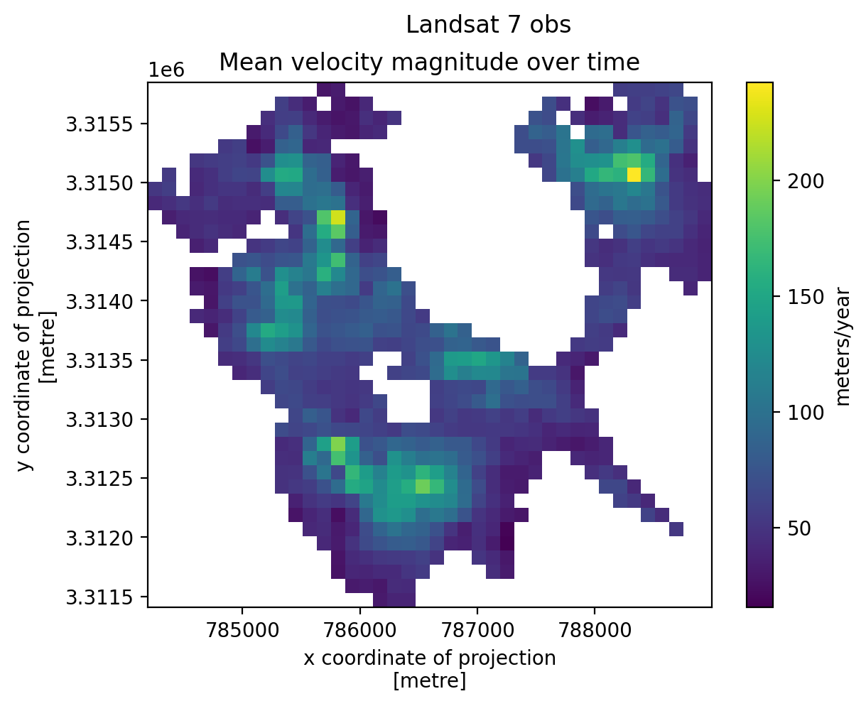
Let’s look at Sentinel 1 data. Note here we are selecting for 2 values instead of 1 using DataArray.isin
s1_condition = sample_glacier_raster.satellite_img1.isin(['1A','1B'])
s1_subset = sample_glacier_raster.sel(mid_date = s1_condition)
s1_subset
<xarray.Dataset> Size: 13MB
Dimensions: (mid_date: 167, y: 37, x: 40)
Coordinates:
* mid_date (mid_date) datetime64[ns] 1kB 2018-12-30T11:4...
* x (x) float64 320B 7.843e+05 ... 7.889e+05
* y (y) float64 296B 3.316e+06 ... 3.311e+06
spatial_ref int64 8B 0
mapping int64 8B 0
Data variables: (12/59)
M11 (mid_date, y, x) float32 989kB nan nan ... nan
M11_dr_to_vr_factor (mid_date) float32 668B nan nan nan ... nan nan
M12 (mid_date, y, x) float32 989kB nan nan ... nan
M12_dr_to_vr_factor (mid_date) float32 668B nan nan nan ... nan nan
acquisition_date_img1 (mid_date) datetime64[ns] 1kB 2018-12-24T11:4...
acquisition_date_img2 (mid_date) datetime64[ns] 1kB 2019-01-05T11:4...
... ...
vy_error_modeled (mid_date) float32 668B 53.7 53.7 ... 53.7 53.7
vy_error_slow (mid_date) float32 668B 55.8 48.2 ... 63.3 54.9
vy_error_stationary (mid_date) float32 668B 55.8 48.2 ... 63.3 54.9
vy_stable_shift (mid_date) float32 668B 0.0 -0.5 ... -0.2 0.0
vy_stable_shift_slow (mid_date) float32 668B 0.0 -0.5 ... -0.2 0.0
vy_stable_shift_stationary (mid_date) float32 668B 0.0 -0.5 ... -0.2 0.0
Attributes: (12/19)
Conventions: CF-1.8
GDAL_AREA_OR_POINT: Area
author: ITS_LIVE, a NASA MEaSUREs project (its-live.j...
autoRIFT_parameter_file: http://its-live-data.s3.amazonaws.com/autorif...
datacube_software_version: 1.0
date_created: 25-Sep-2023 22:00:23
... ...
s3: s3://its-live-data/datacubes/v2/N30E090/ITS_L...
skipped_granules: s3://its-live-data/datacubes/v2/N30E090/ITS_L...
time_standard_img1: UTC
time_standard_img2: UTC
title: ITS_LIVE datacube of image pair velocities
url: https://its-live-data.s3.amazonaws.com/datacu...- mid_date: 167
- y: 37
- x: 40
- mid_date(mid_date)datetime64[ns]2018-12-30T11:41:57.924238080 .....
- description :
- midpoint of image 1 and image 2 acquisition date and time with granule's centroid longitude and latitude as microseconds
- standard_name :
- image_pair_center_date_with_time_separation
array(['2018-12-30T11:41:57.924238080', '2019-09-03T23:37:53.252933888', '2018-03-24T23:37:38.564024320', '2019-04-29T11:41:33.018919936', '2018-02-21T11:41:49.977771008', '2018-05-23T23:37:41.102891008', '2018-04-17T23:37:39.383714048', '2018-08-15T23:37:46.088121344', '2017-11-12T23:37:41.303774976', '2019-12-01T11:42:05.495156992', '2018-09-01T11:41:33.925967616', '2019-04-29T11:41:57.842845952', '2019-02-28T11:41:56.439806976', '2017-12-23T11:41:51.611907072', '2018-01-28T11:41:50.341588736', '2019-02-16T11:41:56.436630016', '2019-10-26T11:42:06.078548992', '2018-06-16T23:37:42.670158080', '2019-12-13T11:42:05.010342912', '2019-05-23T11:41:58.880128000', '2017-06-09T23:37:35.864834048', '2017-11-05T11:41:28.278182912', '2018-12-18T11:41:58.300525056', '2019-11-02T23:37:54.475997952', '2018-11-12T11:41:59.588342016', '2018-07-22T23:37:44.752803072', '2018-05-28T11:41:53.057125888', '2018-03-17T11:41:50.025207040', '2019-02-28T11:41:31.615368192', '2018-06-09T11:41:53.814907904', '2019-02-04T11:41:56.750320896', '2018-09-25T11:41:59.442665984', '2019-11-07T11:41:41.297213952', '2018-11-19T23:37:47.704424960', '2019-07-22T11:42:02.434277120', '2019-08-22T23:37:52.733805056', '2019-10-14T11:42:06.034916096', '2018-09-13T11:41:34.400966912', '2018-10-31T11:41:59.755574016', '2018-07-15T11:41:31.106160128', '2018-04-05T23:37:38.927213056', '2017-07-15T23:37:37.866387968', '2018-01-16T11:41:50.733541888', '2018-03-29T11:41:50.228250112', '2019-09-08T11:42:05.127362048', '2019-03-12T11:41:56.430138112', '2019-03-12T11:41:31.606725888', '2019-06-04T11:41:59.417260032', '2018-04-10T11:41:25.807802112', '2018-02-04T23:37:38.580688896', '2019-01-06T23:37:46.074821120', '2017-10-24T11:41:53.235844096', '2018-12-06T11:41:33.853928192', '2017-03-10T11:41:24.531013888', '2018-10-26T23:37:48.246420736', '2019-01-30T23:37:45.161125376', '2018-04-22T11:41:51.184887040', '2019-04-05T11:41:32.092100352', '2017-02-14T11:41:31.054558976', '2018-01-04T11:41:51.124605952', '2019-03-24T11:41:56.627609088', '2018-07-03T11:41:55.209844224', '2019-09-20T11:42:05.674106880', '2018-12-13T23:37:46.950547968', '2018-08-08T11:41:57.324167936', '2018-08-27T23:37:46.829088000', '2017-09-18T11:41:27.763760128', '2019-11-19T11:41:41.106263040', '2019-04-17T11:41:32.499998976', '2018-07-27T11:41:56.653082112', '2017-04-22T23:37:33.223821056', '2018-04-10T11:41:50.633784320', '2018-12-25T23:37:46.508174848', '2017-07-08T11:41:49.124670208', '2017-07-20T11:41:49.862352896', '2018-04-22T11:41:26.360446976', '2017-04-03T11:41:44.025274112', '2017-12-23T11:41:26.786955008', '2018-03-29T11:41:25.402782976', '2019-01-18T23:37:45.668065792', '2019-08-03T11:42:03.268125952', '2019-12-20T23:37:53.139560960', '2019-10-02T11:42:06.019076352', '2017-11-29T11:41:52.454964224', '2019-04-05T11:41:56.916538624', '2019-07-10T11:42:01.691311872', '2017-05-28T23:37:35.128368640', '2019-08-27T11:41:39.823414016', '2017-11-05T11:41:53.099537920', '2018-06-21T11:41:54.604439040', '2019-05-11T11:41:58.314996992', '2019-10-26T11:41:41.252053760', '2018-07-15T11:41:55.931112960', '2018-05-16T11:41:52.419403008', '2018-06-04T23:37:41.862818304', '2019-10-09T23:37:54.464960256', '2017-10-12T11:41:53.112715008', '2017-04-10T23:37:32.733376000', '2019-06-16T11:42:00.115079936', '2017-08-13T11:41:51.189140992', '2017-05-09T11:41:45.825836032', '2017-03-10T11:41:36.942978048', '2017-12-06T23:37:40.678709760', '2017-03-17T23:37:31.882273792', '2019-11-26T23:37:53.974541056', '2019-08-15T11:42:04.075201024', '2017-05-21T11:41:21.530678016', '2017-09-30T11:41:52.889129984', '2018-10-19T11:41:59.849235968', '2017-10-24T11:41:28.410891776', '2019-11-19T11:42:05.932244992', '2018-08-08T11:41:32.499727872', '2018-01-04T11:41:26.299654144', '2018-09-13T11:41:59.223865088', '2018-09-20T23:37:47.716177152', '2019-09-27T23:37:54.287362816', '2019-11-07T11:42:06.122681088', '2019-12-25T11:42:04.512456960', '2019-01-23T11:41:32.389010944', '2019-08-27T11:42:04.648368128', '2017-02-26T11:41:30.420127232', '2018-12-06T11:41:58.676313088', '2017-12-11T11:41:52.045748992', '2019-09-15T23:37:53.812195072', '2019-07-10T11:41:36.866359040', '2019-11-14T23:37:54.364015104', '2017-05-21T11:41:46.357173760', '2019-06-28T11:42:00.911909120', '2017-11-17T11:41:52.819232000', '2018-11-07T23:37:48.055180288', '2017-03-29T23:37:32.204541952', '2018-09-08T23:37:47.394586880', '2017-08-01T11:41:50.571265024', '2017-03-22T11:41:43.650596352', '2018-02-09T11:41:25.250663168', '2018-05-16T11:41:27.595991040', '2017-04-27T11:41:20.378429952', '2018-11-24T11:41:59.220183040', '2017-02-02T11:41:31.721573120', '2017-11-24T23:37:41.066265088', '2017-04-27T11:41:45.202870016', '2019-01-23T11:41:57.213449728', '2018-08-20T11:41:33.252745984', '2018-02-09T11:41:50.076130048', '2018-08-03T23:37:45.417901056', '2019-02-11T23:37:47.134389760', '2019-02-04T11:41:31.924854016', '2018-09-25T11:41:34.617198080', '2019-10-21T23:37:54.430170112', '2017-09-06T11:41:52.216432896', '2019-01-11T11:41:57.521125120', '2018-03-05T11:41:49.970988032', '2018-04-29T23:37:39.888431104', '2018-10-07T11:41:59.696813056', '2019-12-08T23:37:53.553250048', '2017-03-22T11:41:18.826670080', '2018-03-12T23:37:38.315841024', '2017-09-13T23:37:40.827760640', '2017-08-25T11:41:51.742906112', '2018-05-11T23:37:40.469989120', '2019-04-17T11:41:57.324439040', '2018-12-01T23:37:47.359770880', '2017-09-18T11:41:52.585116928', '2018-05-04T11:41:51.785919232', '2018-07-10T23:37:43.923248128', '2017-04-15T11:41:44.592363008', '2018-06-28T23:37:43.224507904'], dtype='datetime64[ns]') - x(x)float647.843e+05 7.844e+05 ... 7.889e+05
- description :
- x coordinate of projection
- standard_name :
- projection_x_coordinate
- axis :
- X
- long_name :
- x coordinate of projection
- units :
- metre
array([784252.5, 784372.5, 784492.5, 784612.5, 784732.5, 784852.5, 784972.5, 785092.5, 785212.5, 785332.5, 785452.5, 785572.5, 785692.5, 785812.5, 785932.5, 786052.5, 786172.5, 786292.5, 786412.5, 786532.5, 786652.5, 786772.5, 786892.5, 787012.5, 787132.5, 787252.5, 787372.5, 787492.5, 787612.5, 787732.5, 787852.5, 787972.5, 788092.5, 788212.5, 788332.5, 788452.5, 788572.5, 788692.5, 788812.5, 788932.5]) - y(y)float643.316e+06 3.316e+06 ... 3.311e+06
- description :
- y coordinate of projection
- standard_name :
- projection_y_coordinate
- axis :
- Y
- long_name :
- y coordinate of projection
- units :
- metre
array([3315787.5, 3315667.5, 3315547.5, 3315427.5, 3315307.5, 3315187.5, 3315067.5, 3314947.5, 3314827.5, 3314707.5, 3314587.5, 3314467.5, 3314347.5, 3314227.5, 3314107.5, 3313987.5, 3313867.5, 3313747.5, 3313627.5, 3313507.5, 3313387.5, 3313267.5, 3313147.5, 3313027.5, 3312907.5, 3312787.5, 3312667.5, 3312547.5, 3312427.5, 3312307.5, 3312187.5, 3312067.5, 3311947.5, 3311827.5, 3311707.5, 3311587.5, 3311467.5]) - spatial_ref()int640
- GeoTransform :
- 784192.5 120.0 0.0 3315847.5 0.0 -120.0
array(0)
- mapping()int640
- crs_wkt :
- PROJCS["WGS 84 / UTM zone 46N",GEOGCS["WGS 84",DATUM["WGS_1984",SPHEROID["WGS 84",6378137,298.257223563,AUTHORITY["EPSG","7030"]],AUTHORITY["EPSG","6326"]],PRIMEM["Greenwich",0,AUTHORITY["EPSG","8901"]],UNIT["degree",0.0174532925199433,AUTHORITY["EPSG","9122"]],AUTHORITY["EPSG","4326"]],PROJECTION["Transverse_Mercator"],PARAMETER["latitude_of_origin",0],PARAMETER["central_meridian",93],PARAMETER["scale_factor",0.9996],PARAMETER["false_easting",500000],PARAMETER["false_northing",0],UNIT["metre",1,AUTHORITY["EPSG","9001"]],AXIS["Easting",EAST],AXIS["Northing",NORTH],AUTHORITY["EPSG","32646"]]
- semi_major_axis :
- 6378137.0
- semi_minor_axis :
- 6356752.314245179
- inverse_flattening :
- 298.257223563
- reference_ellipsoid_name :
- WGS 84
- longitude_of_prime_meridian :
- 0.0
- prime_meridian_name :
- Greenwich
- geographic_crs_name :
- WGS 84
- horizontal_datum_name :
- World Geodetic System 1984
- projected_crs_name :
- WGS 84 / UTM zone 46N
- grid_mapping_name :
- transverse_mercator
- latitude_of_projection_origin :
- 0.0
- longitude_of_central_meridian :
- 93.0
- false_easting :
- 500000.0
- false_northing :
- 0.0
- scale_factor_at_central_meridian :
- 0.9996
- spatial_ref :
- PROJCS["WGS 84 / UTM zone 46N",GEOGCS["WGS 84",DATUM["WGS_1984",SPHEROID["WGS 84",6378137,298.257223563,AUTHORITY["EPSG","7030"]],AUTHORITY["EPSG","6326"]],PRIMEM["Greenwich",0,AUTHORITY["EPSG","8901"]],UNIT["degree",0.0174532925199433,AUTHORITY["EPSG","9122"]],AUTHORITY["EPSG","4326"]],PROJECTION["Transverse_Mercator"],PARAMETER["latitude_of_origin",0],PARAMETER["central_meridian",93],PARAMETER["scale_factor",0.9996],PARAMETER["false_easting",500000],PARAMETER["false_northing",0],UNIT["metre",1,AUTHORITY["EPSG","9001"]],AXIS["Easting",EAST],AXIS["Northing",NORTH],AUTHORITY["EPSG","32646"]]
- GeoTransform :
- 784192.5 120.0 0.0 3315847.5 0.0 -120.0
array(0)
- M11(mid_date, y, x)float32nan nan nan nan ... nan nan nan nan
- description :
- conversion matrix element (1st row, 1st column) that can be multiplied with vx to give range pixel displacement dr (see Eq. A18 in https://www.mdpi.com/2072-4292/13/4/749)
- standard_name :
- conversion_matrix_element_11
- units :
- pixel/(meter/year)
array([[[nan, nan, nan, ..., nan, nan, nan], [nan, nan, nan, ..., nan, nan, nan], [nan, nan, nan, ..., nan, nan, nan], ..., [nan, nan, nan, ..., nan, nan, nan], [nan, nan, nan, ..., nan, nan, nan], [nan, nan, nan, ..., nan, nan, nan]], [[nan, nan, nan, ..., nan, nan, nan], [nan, nan, nan, ..., 0., 0., nan], [nan, nan, nan, ..., 0., 0., nan], ..., [nan, nan, nan, ..., nan, nan, nan], [nan, nan, nan, ..., nan, nan, nan], [nan, nan, nan, ..., nan, nan, nan]], [[nan, nan, nan, ..., 0., nan, nan], [nan, nan, nan, ..., 0., 0., nan], [nan, nan, nan, ..., 0., 0., nan], ..., ... [nan, nan, nan, ..., nan, nan, nan], [nan, nan, nan, ..., nan, nan, nan], [nan, nan, nan, ..., nan, nan, nan]], [[nan, nan, nan, ..., nan, nan, nan], [nan, nan, nan, ..., nan, nan, nan], [nan, nan, nan, ..., nan, nan, nan], ..., [nan, nan, nan, ..., nan, nan, nan], [nan, nan, nan, ..., nan, nan, nan], [nan, nan, nan, ..., nan, nan, nan]], [[nan, nan, nan, ..., 0., nan, nan], [nan, nan, nan, ..., 0., 0., nan], [nan, nan, nan, ..., 0., 0., nan], ..., [nan, nan, nan, ..., nan, nan, nan], [nan, nan, nan, ..., nan, nan, nan], [nan, nan, nan, ..., nan, nan, nan]]], shape=(167, 37, 40), dtype=float32) - M11_dr_to_vr_factor(mid_date)float32nan nan nan nan ... nan nan nan nan
- description :
- multiplicative factor that converts slant range pixel displacement dr to slant range velocity vr
- standard_name :
- M11_dr_to_vr_factor
- units :
- meter/(year*pixel)
array([nan, nan, nan, nan, nan, nan, nan, nan, nan, nan, nan, nan, nan, nan, nan, nan, nan, nan, nan, nan, nan, nan, nan, nan, nan, nan, nan, nan, nan, nan, nan, nan, nan, nan, nan, nan, nan, nan, nan, nan, nan, nan, nan, nan, nan, nan, nan, nan, nan, nan, nan, nan, nan, nan, nan, nan, nan, nan, nan, nan, nan, nan, nan, nan, nan, nan, nan, nan, nan, nan, nan, nan, nan, nan, nan, nan, nan, nan, nan, nan, nan, nan, nan, nan, nan, nan, nan, nan, nan, nan, nan, nan, nan, nan, nan, nan, nan, nan, nan, nan, nan, nan, nan, nan, nan, nan, nan, nan, nan, nan, nan, nan, nan, nan, nan, nan, nan, nan, nan, nan, nan, nan, nan, nan, nan, nan, nan, nan, nan, nan, nan, nan, nan, nan, nan, nan, nan, nan, nan, nan, nan, nan, nan, nan, nan, nan, nan, nan, nan, nan, nan, nan, nan, nan, nan, nan, nan, nan, nan, nan, nan, nan, nan, nan, nan, nan, nan], dtype=float32) - M12(mid_date, y, x)float32nan nan nan nan ... nan nan nan nan
- description :
- conversion matrix element (1st row, 2nd column) that can be multiplied with vy to give range pixel displacement dr (see Eq. A18 in https://www.mdpi.com/2072-4292/13/4/749)
- standard_name :
- conversion_matrix_element_12
- units :
- pixel/(meter/year)
array([[[nan, nan, nan, ..., nan, nan, nan], [nan, nan, nan, ..., nan, nan, nan], [nan, nan, nan, ..., nan, nan, nan], ..., [nan, nan, nan, ..., nan, nan, nan], [nan, nan, nan, ..., nan, nan, nan], [nan, nan, nan, ..., nan, nan, nan]], [[nan, nan, nan, ..., nan, nan, nan], [nan, nan, nan, ..., 0., 0., nan], [nan, nan, nan, ..., 0., 0., nan], ..., [nan, nan, nan, ..., nan, nan, nan], [nan, nan, nan, ..., nan, nan, nan], [nan, nan, nan, ..., nan, nan, nan]], [[nan, nan, nan, ..., 0., nan, nan], [nan, nan, nan, ..., 0., 0., nan], [nan, nan, nan, ..., 0., 0., nan], ..., ... [nan, nan, nan, ..., nan, nan, nan], [nan, nan, nan, ..., nan, nan, nan], [nan, nan, nan, ..., nan, nan, nan]], [[nan, nan, nan, ..., nan, nan, nan], [nan, nan, nan, ..., nan, nan, nan], [nan, nan, nan, ..., nan, nan, nan], ..., [nan, nan, nan, ..., nan, nan, nan], [nan, nan, nan, ..., nan, nan, nan], [nan, nan, nan, ..., nan, nan, nan]], [[nan, nan, nan, ..., 0., nan, nan], [nan, nan, nan, ..., 0., 0., nan], [nan, nan, nan, ..., 0., 0., nan], ..., [nan, nan, nan, ..., nan, nan, nan], [nan, nan, nan, ..., nan, nan, nan], [nan, nan, nan, ..., nan, nan, nan]]], shape=(167, 37, 40), dtype=float32) - M12_dr_to_vr_factor(mid_date)float32nan nan nan nan ... nan nan nan nan
- description :
- multiplicative factor that converts slant range pixel displacement dr to slant range velocity vr
- standard_name :
- M12_dr_to_vr_factor
- units :
- meter/(year*pixel)
array([nan, nan, nan, nan, nan, nan, nan, nan, nan, nan, nan, nan, nan, nan, nan, nan, nan, nan, nan, nan, nan, nan, nan, nan, nan, nan, nan, nan, nan, nan, nan, nan, nan, nan, nan, nan, nan, nan, nan, nan, nan, nan, nan, nan, nan, nan, nan, nan, nan, nan, nan, nan, nan, nan, nan, nan, nan, nan, nan, nan, nan, nan, nan, nan, nan, nan, nan, nan, nan, nan, nan, nan, nan, nan, nan, nan, nan, nan, nan, nan, nan, nan, nan, nan, nan, nan, nan, nan, nan, nan, nan, nan, nan, nan, nan, nan, nan, nan, nan, nan, nan, nan, nan, nan, nan, nan, nan, nan, nan, nan, nan, nan, nan, nan, nan, nan, nan, nan, nan, nan, nan, nan, nan, nan, nan, nan, nan, nan, nan, nan, nan, nan, nan, nan, nan, nan, nan, nan, nan, nan, nan, nan, nan, nan, nan, nan, nan, nan, nan, nan, nan, nan, nan, nan, nan, nan, nan, nan, nan, nan, nan, nan, nan, nan, nan, nan, nan], dtype=float32) - acquisition_date_img1(mid_date)datetime64[ns]2018-12-24T11:41:58.030734080 .....
- description :
- acquisition date and time of image 1
- standard_name :
- image1_acquition_date
array(['2018-12-24T11:41:58.030734080', '2019-08-28T23:37:52.754460160', '2018-03-18T23:37:38.228302080', '2019-04-23T11:41:32.673425152', '2018-02-15T11:41:49.810621696', '2018-05-17T23:37:40.614904320', '2018-04-11T23:37:38.954653952', '2018-08-09T23:37:45.571847936', '2017-11-06T23:37:41.213552896', '2019-11-25T11:42:05.563342080', '2018-08-26T11:41:33.424268032', '2019-04-23T11:41:57.497350912', '2019-02-22T11:41:56.212375040', '2017-12-17T11:41:51.739784960', '2018-01-22T11:41:50.341702912', '2019-02-10T11:41:56.280463872', '2019-10-20T11:42:05.830819072', '2018-06-10T23:37:42.134734080', '2019-12-07T11:42:05.044720896', '2019-05-17T11:41:58.441488896', '2017-06-03T23:37:35.380610048', '2017-10-30T11:41:28.296257024', '2018-12-12T11:41:58.207891968', '2019-10-27T23:37:54.250460928', '2018-11-06T11:41:59.518813952', '2018-07-16T23:37:44.241677056', '2018-05-22T11:41:52.572083968', '2018-03-11T11:41:49.797033984', '2019-02-22T11:41:31.388447744', '2018-06-03T11:41:53.181125120', '2019-01-29T11:41:56.839920128', '2018-09-19T11:41:59.198030848', '2019-11-01T11:41:41.117229312', '2018-11-13T23:37:47.730641920', '2019-07-16T11:42:01.891853056', '2019-08-16T23:37:52.331518976', '2019-10-08T11:42:05.856997888', '2018-09-07T11:41:34.066016000', '2018-10-25T11:41:59.630284032', '2018-07-09T11:41:30.473315072', ... '2017-11-11T11:41:52.737861888', '2018-11-01T23:37:48.017517056', '2017-03-23T23:37:31.793750016', '2018-09-02T23:37:47.053758976', '2017-07-26T11:41:50.082296064', '2017-03-16T11:41:43.372389888', '2018-02-03T11:41:25.154222848', '2018-05-10T11:41:27.082804992', '2017-04-21T11:41:19.897232896', '2018-11-18T11:41:59.295656960', '2017-01-27T11:41:31.661045760', '2017-11-18T23:37:41.051783936', '2017-04-21T11:41:44.722187008', '2019-01-17T11:41:57.206746880', '2018-08-14T11:41:32.719596032', '2018-02-03T11:41:49.981231872', '2018-07-28T23:37:44.902497024', '2019-02-05T23:37:44.616735232', '2019-01-29T11:41:32.014967040', '2018-09-19T11:41:34.374105088', '2019-10-15T23:37:54.227848960', '2017-08-31T11:41:51.826288896', '2019-01-05T11:41:57.455292672', '2018-02-27T11:41:49.784488704', '2018-04-23T23:37:39.451952128', '2018-10-01T11:41:59.325461760', '2019-12-02T23:37:53.540507904', '2017-03-16T11:41:18.548463104', '2018-03-06T23:37:38.042767872', '2017-09-07T23:37:40.395532032', '2017-08-19T11:41:51.317884928', '2018-05-05T23:37:39.964064000', '2019-04-11T11:41:56.770703872', '2018-11-25T23:37:47.315982080', '2017-09-12T11:41:52.264914944', '2018-04-28T11:41:51.305278976', '2018-07-04T23:37:43.243410176', '2017-04-09T11:41:44.121721344', '2018-06-22T23:37:42.844361984'], dtype='datetime64[ns]') - acquisition_date_img2(mid_date)datetime64[ns]2019-01-05T11:41:57.455292672 .....
- description :
- acquisition date and time of image 2
- standard_name :
- image2_acquition_date
array(['2019-01-05T11:41:57.455292672', '2019-09-09T23:37:53.369752064', '2018-03-30T23:37:38.539110912', '2019-05-05T11:41:32.983569920', '2018-02-27T11:41:49.784488704', '2018-05-29T23:37:41.229844992', '2018-04-23T23:37:39.451952128', '2018-08-21T23:37:46.242775296', '2017-11-18T23:37:41.051783936', '2019-12-07T11:42:05.044720896', '2018-09-07T11:41:34.066016000', '2019-05-05T11:41:57.807494912', '2019-03-06T11:41:56.286795776', '2017-12-29T11:41:51.141594880', '2018-02-03T11:41:49.981231872', '2019-02-22T11:41:56.212375040', '2019-11-01T11:42:05.944238336', '2018-06-22T23:37:42.844361984', '2019-12-19T11:42:04.593551104', '2019-05-29T11:41:58.937733888', '2017-06-15T23:37:36.007851776', '2017-11-11T11:41:27.918048000', '2018-12-24T11:41:58.030734080', '2019-11-08T23:37:54.319481344', '2018-11-18T11:41:59.295656960', '2018-07-28T23:37:44.902497024', '2018-06-03T11:41:53.181125120', '2018-03-23T11:41:49.892759040', '2019-03-06T11:41:31.461842944', '2018-06-15T11:41:54.087483904', '2019-02-10T11:41:56.280463872', '2018-10-01T11:41:59.325461760', '2019-11-13T11:41:41.094995968', '2018-11-25T23:37:47.315982080', '2019-07-28T11:42:02.595268096', '2019-08-28T23:37:52.754460160', '2019-10-20T11:42:05.830819072', '2018-09-19T11:41:34.374105088', '2018-11-06T11:41:59.518813952', '2018-07-21T11:41:31.377586688', ... '2017-11-23T11:41:52.558380032', '2018-11-13T23:37:47.730641920', '2017-04-04T23:37:32.274688000', '2018-09-14T23:37:47.373610240', '2017-08-07T11:41:50.718781952', '2017-03-28T11:41:43.588171008', '2018-02-15T11:41:24.986696960', '2018-05-22T11:41:27.748157952', '2017-05-03T11:41:20.518784000', '2018-11-30T11:41:58.782473984', '2017-02-08T11:41:31.441846016', '2017-11-30T23:37:40.738510080', '2017-05-03T11:41:45.342711040', '2019-01-29T11:41:56.839920128', '2018-08-26T11:41:33.424268032', '2018-02-15T11:41:49.810621696', '2018-08-09T23:37:45.571847936', '2019-02-17T23:37:49.271634944', '2019-02-10T11:41:31.454482944', '2018-10-01T11:41:34.498452736', '2019-10-27T23:37:54.250460928', '2017-09-12T11:41:52.264914944', '2019-01-17T11:41:57.206746880', '2018-03-11T11:41:49.797033984', '2018-05-05T23:37:39.964064000', '2018-10-13T11:41:59.706161920', '2019-12-14T23:37:53.183587072', '2017-03-28T11:41:18.764244992', '2018-03-18T23:37:38.228302080', '2017-09-19T23:37:40.918177280', '2017-08-31T11:41:51.826288896', '2018-05-17T23:37:40.614904320', '2019-04-23T11:41:57.497350912', '2018-12-07T23:37:47.041310720', '2017-09-24T11:41:52.563493888', '2018-05-10T11:41:51.905702912', '2018-07-16T23:37:44.241677056', '2017-04-21T11:41:44.722187008', '2018-07-04T23:37:43.243410176'], dtype='datetime64[ns]') - autoRIFT_software_version(mid_date)object'1.4.0' '1.4.0' ... '1.4.0' '1.4.0'
- description :
- version of autoRIFT software
- standard_name :
- autoRIFT_software_version
array(['1.4.0', '1.4.0', '1.4.0', '1.4.0', '1.4.0', '1.4.0', '1.4.0', '1.4.0', '1.4.0', '1.4.0', '1.4.0', '1.4.0', '1.4.0', '1.4.0', '1.4.0', '1.4.0', '1.4.0', '1.4.0', '1.4.0', '1.4.0', '1.4.0', '1.4.0', '1.4.0', '1.4.0', '1.4.0', '1.4.0', '1.4.0', '1.4.0', '1.4.0', '1.4.0', '1.4.0', '1.4.0', '1.4.0', '1.4.0', '1.4.0', '1.4.0', '1.4.0', '1.4.0', '1.4.0', '1.4.0', '1.4.0', '1.4.0', '1.4.0', '1.4.0', '1.4.0', '1.4.0', '1.4.0', '1.4.0', '1.4.0', '1.4.0', '1.4.0', '1.4.0', '1.4.0', '1.4.0', '1.4.0', '1.4.0', '1.4.0', '1.4.0', '1.4.0', '1.4.0', '1.4.0', '1.4.0', '1.4.0', '1.4.0', '1.4.0', '1.4.0', '1.4.0', '1.4.0', '1.4.0', '1.4.0', '1.4.0', '1.4.0', '1.4.0', '1.4.0', '1.4.0', '1.4.0', '1.4.0', '1.4.0', '1.4.0', '1.4.0', '1.4.0', '1.4.0', '1.4.0', '1.4.0', '1.4.0', '1.4.0', '1.4.0', '1.4.0', '1.4.0', '1.4.0', '1.4.0', '1.4.0', '1.4.0', '1.4.0', '1.4.0', '1.4.0', '1.4.0', '1.4.0', '1.4.0', '1.4.0', '1.4.0', '1.4.0', '1.4.0', '1.4.0', '1.4.0', '1.4.0', '1.4.0', '1.4.0', '1.4.0', '1.4.0', '1.4.0', '1.4.0', '1.4.0', '1.4.0', '1.4.0', '1.4.0', '1.4.0', '1.4.0', '1.4.0', '1.4.0', '1.4.0', '1.4.0', '1.4.0', '1.4.0', '1.4.0', '1.4.0', '1.4.0', '1.4.0', '1.4.0', '1.4.0', '1.4.0', '1.4.0', '1.4.0', '1.4.0', '1.4.0', '1.4.0', '1.4.0', '1.4.0', '1.4.0', '1.4.0', '1.4.0', '1.4.0', '1.4.0', '1.4.0', '1.4.0', '1.4.0', '1.4.0', '1.4.0', '1.4.0', '1.4.0', '1.4.0', '1.4.0', '1.4.0', '1.4.0', '1.4.0', '1.4.0', '1.4.0', '1.4.0', '1.4.0', '1.4.0', '1.4.0', '1.4.0', '1.4.0', '1.4.0', '1.4.0', '1.4.0', '1.4.0'], dtype=object) - chip_size_height(mid_date, y, x)float32nan nan nan nan ... nan nan nan nan
- chip_size_coordinates :
- Optical data: chip_size_coordinates = 'image projection geometry: width = x, height = y'. Radar data: chip_size_coordinates = 'radar geometry: width = range, height = azimuth'
- description :
- height of search template (chip)
- standard_name :
- chip_size_height
- units :
- m
- y_pixel_size :
- 10.0
array([[[ nan, nan, nan, ..., nan, nan, nan], [ nan, nan, nan, ..., nan, nan, nan], [ nan, nan, nan, ..., nan, nan, nan], ..., [ nan, nan, nan, ..., nan, nan, nan], [ nan, nan, nan, ..., nan, nan, nan], [ nan, nan, nan, ..., nan, nan, nan]], [[ nan, nan, nan, ..., nan, nan, nan], [ nan, nan, nan, ..., 223., 223., nan], [ nan, nan, nan, ..., 223., 223., nan], ..., [ nan, nan, nan, ..., nan, nan, nan], [ nan, nan, nan, ..., nan, nan, nan], [ nan, nan, nan, ..., nan, nan, nan]], [[ nan, nan, nan, ..., 223., nan, nan], [ nan, nan, nan, ..., 223., 223., nan], [ nan, nan, nan, ..., 223., 223., nan], ..., ... [ nan, nan, nan, ..., nan, nan, nan], [ nan, nan, nan, ..., nan, nan, nan], [ nan, nan, nan, ..., nan, nan, nan]], [[ nan, nan, nan, ..., nan, nan, nan], [ nan, nan, nan, ..., nan, nan, nan], [ nan, nan, nan, ..., nan, nan, nan], ..., [ nan, nan, nan, ..., nan, nan, nan], [ nan, nan, nan, ..., nan, nan, nan], [ nan, nan, nan, ..., nan, nan, nan]], [[ nan, nan, nan, ..., 223., nan, nan], [ nan, nan, nan, ..., 223., 223., nan], [ nan, nan, nan, ..., 223., 223., nan], ..., [ nan, nan, nan, ..., nan, nan, nan], [ nan, nan, nan, ..., nan, nan, nan], [ nan, nan, nan, ..., nan, nan, nan]]], shape=(167, 37, 40), dtype=float32) - chip_size_width(mid_date, y, x)float32nan nan nan nan ... nan nan nan nan
- chip_size_coordinates :
- Optical data: chip_size_coordinates = 'image projection geometry: width = x, height = y'. Radar data: chip_size_coordinates = 'radar geometry: width = range, height = azimuth'
- description :
- width of search template (chip)
- standard_name :
- chip_size_width
- units :
- m
- x_pixel_size :
- 10.0
array([[[ nan, nan, nan, ..., nan, nan, nan], [ nan, nan, nan, ..., nan, nan, nan], [ nan, nan, nan, ..., nan, nan, nan], ..., [ nan, nan, nan, ..., nan, nan, nan], [ nan, nan, nan, ..., nan, nan, nan], [ nan, nan, nan, ..., nan, nan, nan]], [[ nan, nan, nan, ..., nan, nan, nan], [ nan, nan, nan, ..., 247., 247., nan], [ nan, nan, nan, ..., 247., 247., nan], ..., [ nan, nan, nan, ..., nan, nan, nan], [ nan, nan, nan, ..., nan, nan, nan], [ nan, nan, nan, ..., nan, nan, nan]], [[ nan, nan, nan, ..., 247., nan, nan], [ nan, nan, nan, ..., 247., 247., nan], [ nan, nan, nan, ..., 247., 247., nan], ..., ... [ nan, nan, nan, ..., nan, nan, nan], [ nan, nan, nan, ..., nan, nan, nan], [ nan, nan, nan, ..., nan, nan, nan]], [[ nan, nan, nan, ..., nan, nan, nan], [ nan, nan, nan, ..., nan, nan, nan], [ nan, nan, nan, ..., nan, nan, nan], ..., [ nan, nan, nan, ..., nan, nan, nan], [ nan, nan, nan, ..., nan, nan, nan], [ nan, nan, nan, ..., nan, nan, nan]], [[ nan, nan, nan, ..., 247., nan, nan], [ nan, nan, nan, ..., 247., 247., nan], [ nan, nan, nan, ..., 247., 247., nan], ..., [ nan, nan, nan, ..., nan, nan, nan], [ nan, nan, nan, ..., nan, nan, nan], [ nan, nan, nan, ..., nan, nan, nan]]], shape=(167, 37, 40), dtype=float32) - date_center(mid_date)datetime64[ns]2018-12-30T11:41:57.743013888 .....
- description :
- midpoint of image 1 and image 2 acquisition date
- standard_name :
- image_pair_center_date
array(['2018-12-30T11:41:57.743013888', '2019-09-03T23:37:53.062106112', '2018-03-24T23:37:38.383706112', '2019-04-29T11:41:32.828496640', '2018-02-21T11:41:49.797555968', '2018-05-23T23:37:40.922373888', '2018-04-17T23:37:39.203302912', '2018-08-15T23:37:45.907312128', '2017-11-12T23:37:41.132668928', '2019-12-01T11:42:05.304032000', '2018-09-01T11:41:33.745142016', '2019-04-29T11:41:57.652422912', '2019-02-28T11:41:56.249584896', '2017-12-23T11:41:51.440689920', '2018-01-28T11:41:50.161466880', '2019-02-16T11:41:56.246419968', '2019-10-26T11:42:05.887528960', '2018-06-16T23:37:42.489548032', '2019-12-13T11:42:04.819136000', '2019-05-23T11:41:58.689611008', '2017-06-09T23:37:35.694231040', '2017-11-05T11:41:28.107152896', '2018-12-18T11:41:58.119313152', '2019-11-02T23:37:54.284971008', '2018-11-12T11:41:59.407236096', '2018-07-22T23:37:44.572087040', '2018-05-28T11:41:52.876603904', '2018-03-17T11:41:49.844896000', '2019-02-28T11:41:31.425146112', '2018-06-09T11:41:53.634305024', '2019-02-04T11:41:56.560192000', '2018-09-25T11:41:59.261746944', '2019-11-07T11:41:41.106113024', '2018-11-19T23:37:47.523312384', '2019-07-22T11:42:02.243560704', '2019-08-22T23:37:52.542989056', '2019-10-14T11:42:05.843908096', '2018-09-13T11:41:34.220059904', '2018-10-31T11:41:59.574548992', '2018-07-15T11:41:30.925451008', ... '2017-11-17T11:41:52.648121088', '2018-11-07T23:37:47.874078976', '2017-03-29T23:37:32.034219008', '2018-09-08T23:37:47.213684992', '2017-08-01T11:41:50.400538880', '2017-03-22T11:41:43.480280064', '2018-02-09T11:41:25.070459904', '2018-05-16T11:41:27.415481088', '2017-04-27T11:41:20.208009216', '2018-11-24T11:41:59.039065088', '2017-02-02T11:41:31.551446016', '2017-11-24T23:37:40.895147264', '2017-04-27T11:41:45.032449280', '2019-01-23T11:41:57.023333120', '2018-08-20T11:41:33.071932160', '2018-02-09T11:41:49.895927040', '2018-08-03T23:37:45.237173248', '2019-02-11T23:37:46.944185088', '2019-02-04T11:41:31.734725120', '2018-09-25T11:41:34.436279040', '2019-10-21T23:37:54.239154944', '2017-09-06T11:41:52.045602048', '2019-01-11T11:41:57.331020288', '2018-03-05T11:41:49.790761216', '2018-04-29T23:37:39.708007936', '2018-10-07T11:41:59.515812096', '2019-12-08T23:37:53.362048000', '2017-03-22T11:41:18.656354048', '2018-03-12T23:37:38.135535104', '2017-09-13T23:37:40.656854272', '2017-08-25T11:41:51.572087040', '2018-05-11T23:37:40.289484032', '2019-04-17T11:41:57.134028032', '2018-12-01T23:37:47.178646016', '2017-09-18T11:41:52.414204672', '2018-05-04T11:41:51.605490688', '2018-07-10T23:37:43.742543872', '2017-04-15T11:41:44.421954048', '2018-06-28T23:37:43.043886080'], dtype='datetime64[ns]') - date_dt(mid_date)timedelta64[ns]11 days 23:59:59.423217774 ... 1...
- description :
- time separation between acquisition of image 1 and image 2
- standard_name :
- image_pair_time_separation
array([1036799423217774, 1036800576782225, 1036800329589846, 1036800329589846, 1036800000000000, 1036800576782225, 1036800494384765, 1036800659179684, 1036799835205080, 1036799505615234, 1036800659179684, 1036800329589846, 1036800082397459, 1036799423217774, 1036799670410153, 1036799917602540, 1036800082397459, 1036800741577144, 1036799588012693, 1036800494384765, 1036800659179684, 1036799588012693, 1036799835205080, 1036800082397459, 1036799752807621, 1036800659179684, 1036800576782225, 1036800082397459, 1036800082397459, 1036800906372072, 1036799423217774, 1036800164794919, 1036800000000000, 1036799588012693, 1036800741577144, 1036800411987306, 1036800000000000, 1036800329589846, 1036799917602540, 1036800906372072, 1036800411987306, 1036800659179684, 1036799588012693, 1036800329589846, 1036800494384765, 1036799917602540, 1036799917602540, 1036800576782225, 1036800494384765, 1036799835205080, 1036799505615234, 1036800082397459, 1036799423217774, 1036788381958008, 1036799917602540, 1036799258422855, 1036800576782225, 1036800082397459, 1036798846435549, 1036799588012693, ... 1036799917602540, 1036800082397459, 1036799670410153, 1036800823974612, 1036799588012693, 1036800329589846, 1036800329589846, 1036800411987306, 1036800000000000, 1036799423217774, 1036799670410153, 1036800494384765, 1036799835205080, 1036799423217774, 1036799752807621, 1036800494384765, 1036800741577144, 1036799670410153, 1036800411987306, 1036800741577144, 1036799835205080, 1036799752807621, 1036800494384765, 1036800329589846, 1036800659179684, 1036800247192378, 1036799835205080, 1036800659179684, 1036800659179684, 1036799505615234, 1036799752807621, 1036799670410153, 1036800659179684, 1036799670410153, 1036800741577144, 1036799835205080, 1036800659179684, 1036804614257810, 1036799423217774, 1036800164794919, 1036800000000000, 1036800411987306, 1036799752807621, 1036800000000000, 1036800494384765, 1036800411987306, 1036799670410153, 1036800247192378, 1036800164794919, 1036800494384765, 1036800494384765, 1036800659179684, 1036800741577144, 1036799752807621, 1036800329589846, 1036800576782225, 1036800988769531, 1036800576782225, 1036800411987306], dtype='timedelta64[ns]') - floatingice(y, x, mid_date)float32nan nan nan nan ... nan nan nan nan
- description :
- floating ice mask, 0 = non-floating-ice, 1 = floating-ice
- flag_meanings :
- non-ice ice
- flag_values :
- [0, 1]
- standard_name :
- floating ice mask
- url :
- https://its-live-data.s3.amazonaws.com/autorift_parameters/v001/N46_0120m_floatingice.tif
array([[[nan, nan, nan, ..., nan, nan, nan], [nan, nan, nan, ..., nan, nan, nan], [nan, nan, nan, ..., nan, nan, nan], ..., [ 0., 0., 0., ..., 0., 0., 0.], [nan, nan, nan, ..., nan, nan, nan], [nan, nan, nan, ..., nan, nan, nan]], [[nan, nan, nan, ..., nan, nan, nan], [nan, nan, nan, ..., nan, nan, nan], [nan, nan, nan, ..., nan, nan, nan], ..., [ 0., 0., 0., ..., 0., 0., 0.], [ 0., 0., 0., ..., 0., 0., 0.], [nan, nan, nan, ..., nan, nan, nan]], [[nan, nan, nan, ..., nan, nan, nan], [nan, nan, nan, ..., nan, nan, nan], [nan, nan, nan, ..., nan, nan, nan], ..., ... [nan, nan, nan, ..., nan, nan, nan], [nan, nan, nan, ..., nan, nan, nan], [nan, nan, nan, ..., nan, nan, nan]], [[nan, nan, nan, ..., nan, nan, nan], [nan, nan, nan, ..., nan, nan, nan], [nan, nan, nan, ..., nan, nan, nan], ..., [nan, nan, nan, ..., nan, nan, nan], [nan, nan, nan, ..., nan, nan, nan], [nan, nan, nan, ..., nan, nan, nan]], [[nan, nan, nan, ..., nan, nan, nan], [nan, nan, nan, ..., nan, nan, nan], [nan, nan, nan, ..., nan, nan, nan], ..., [nan, nan, nan, ..., nan, nan, nan], [nan, nan, nan, ..., nan, nan, nan], [nan, nan, nan, ..., nan, nan, nan]]], shape=(37, 40, 167), dtype=float32) - granule_url(mid_date)object'https://its-live-data.s3.amazon...
- description :
- original granule URL
- standard_name :
- granule_url
array(['https://its-live-data.s3.amazonaws.com/velocity_image_pair/sentinel1/v02/N30E090/S1A_IW_SLC__1SDV_20181224T114144_20181224T114211_025167_02C7BC_E321_X_S1A_IW_SLC__1SDV_20190105T114143_20190105T114210_025342_02CE0B_D3E7_G0120V02_P098.nc', 'https://its-live-data.s3.amazonaws.com/velocity_image_pair/sentinel1/v02/N30E090/S1A_IW_SLC__1SDV_20190828T233739_20190828T233806_028776_03425A_5628_X_S1A_IW_SLC__1SDV_20190909T233739_20190909T233806_028951_03486D_F888_G0120V02_P097.nc', 'https://its-live-data.s3.amazonaws.com/velocity_image_pair/sentinel1/v02/N30E090/S1A_IW_SLC__1SDV_20180318T233724_20180318T233751_021076_024341_17A7_X_S1A_IW_SLC__1SDV_20180330T233725_20180330T233752_021251_0248CF_4746_G0120V02_P097.nc', 'https://its-live-data.s3.amazonaws.com/velocity_image_pair/sentinel1/v02/N20E090/S1A_IW_SLC__1SDV_20190423T114119_20190423T114146_026917_03072B_D471_X_S1A_IW_SLC__1SDV_20190505T114119_20190505T114146_027092_030D8B_52FA_G0120V02_P095.nc', 'https://its-live-data.s3.amazonaws.com/velocity_image_pair/sentinel1/v02/N30E090/S1A_IW_SLC__1SDV_20180215T114136_20180215T114203_020617_0234C0_E91F_X_S1A_IW_SLC__1SDV_20180227T114136_20180227T114203_020792_023A5A_3A59_G0120V02_P098.nc', 'https://its-live-data.s3.amazonaws.com/velocity_image_pair/sentinel1/v02/N30E090/S1A_IW_SLC__1SDV_20180517T233727_20180517T233754_021951_025ED2_2BFA_X_S1A_IW_SLC__1SDV_20180529T233727_20180529T233754_022126_026474_E4C7_G0120V02_P094.nc', 'https://its-live-data.s3.amazonaws.com/velocity_image_pair/sentinel1/v02/N30E090/S1A_IW_SLC__1SDV_20180411T233725_20180411T233752_021426_024E48_F035_X_S1A_IW_SLC__1SDV_20180423T233725_20180423T233752_021601_0253B9_A996_G0120V02_P096.nc', 'https://its-live-data.s3.amazonaws.com/velocity_image_pair/sentinel1/v02/N30E090/S1A_IW_SLC__1SDV_20180809T233732_20180809T233759_023176_028494_6490_X_S1A_IW_SLC__1SDV_20180821T233732_20180821T233759_023351_028A3F_83CC_G0120V02_P097.nc', 'https://its-live-data.s3.amazonaws.com/velocity_image_pair/sentinel1/v02/N30E090/S1A_IW_SLC__1SDV_20171106T233727_20171106T233754_019151_02068B_355B_X_S1A_IW_SLC__1SDV_20171118T233727_20171118T233754_019326_020C05_F81A_G0120V02_P098.nc', 'https://its-live-data.s3.amazonaws.com/velocity_image_pair/sentinel1/v02/N30E090/S1A_IW_SLC__1SDV_20191125T114152_20191125T114219_030067_036F15_5A87_X_S1A_IW_SLC__1SDV_20191207T114151_20191207T114218_030242_037518_6A21_G0120V02_P098.nc', 'https://its-live-data.s3.amazonaws.com/velocity_image_pair/sentinel1/v02/N20E090/S1A_IW_SLC__1SDV_20180826T114119_20180826T114146_023417_028C5A_F7CA_X_S1A_IW_SLC__1SDV_20180907T114120_20180907T114147_023592_0291F1_8507_G0120V02_P097.nc', 'https://its-live-data.s3.amazonaws.com/velocity_image_pair/sentinel1/v02/N30E090/S1A_IW_SLC__1SDV_20190423T114144_20190423T114210_026917_03072B_4C79_X_S1A_IW_SLC__1SDV_20190505T114144_20190505T114211_027092_030D8B_CB36_G0120V02_P095.nc', 'https://its-live-data.s3.amazonaws.com/velocity_image_pair/sentinel1/v02/N30E090/S1A_IW_SLC__1SDV_20190222T114142_20190222T114209_026042_02E742_8210_X_S1A_IW_SLC__1SDV_20190306T114142_20190306T114209_026217_02ED85_C180_G0120V02_P097.nc', 'https://its-live-data.s3.amazonaws.com/velocity_image_pair/sentinel1/v02/N30E090/S1A_IW_SLC__1SDV_20171217T114138_20171217T114205_019742_021916_4A54_X_S1A_IW_SLC__1SDV_20171229T114137_20171229T114204_019917_021E81_F442_G0120V02_P099.nc', 'https://its-live-data.s3.amazonaws.com/velocity_image_pair/sentinel1/v02/N30E090/S1A_IW_SLC__1SDV_20180122T114136_20180122T114203_020267_022997_E449_X_S1A_IW_SLC__1SDV_20180203T114136_20180203T114203_020442_022F2D_75DE_G0120V02_P098.nc', 'https://its-live-data.s3.amazonaws.com/velocity_image_pair/sentinel1/v02/N30E090/S1A_IW_SLC__1SDV_20190210T114142_20190210T114209_025867_02E10F_A144_X_S1A_IW_SLC__1SDV_20190222T114142_20190222T114209_026042_02E742_8210_G0120V02_P097.nc', 'https://its-live-data.s3.amazonaws.com/velocity_image_pair/sentinel1/v02/N30E090/S1A_IW_SLC__1SDV_20191020T114152_20191020T114219_029542_035CCA_CB77_X_S1A_IW_SLC__1SDV_20191101T114152_20191101T114219_029717_0362E0_1EB7_G0120V02_P097.nc', 'https://its-live-data.s3.amazonaws.com/velocity_image_pair/sentinel1/v02/N30E090/S1A_IW_SLC__1SDV_20180610T233728_20180610T233755_022301_0269E9_F935_X_S1A_IW_SLC__1SDV_20180622T233729_20180622T233756_022476_026F2D_1CB4_G0120V02_P097.nc', 'https://its-live-data.s3.amazonaws.com/velocity_image_pair/sentinel1/v02/N30E090/S1A_IW_SLC__1SDV_20191207T114151_20191207T114218_030242_037518_6A21_X_S1A_IW_SLC__1SDV_20191219T114151_20191219T114218_030417_037B24_43A4_G0120V02_P098.nc', 'https://its-live-data.s3.amazonaws.com/velocity_image_pair/sentinel1/v02/N30E090/S1A_IW_SLC__1SDV_20190517T114144_20190517T114211_027267_031314_C4CE_X_S1A_IW_SLC__1SDV_20190529T114145_20190529T114212_027442_03188B_BE30_G0120V02_P097.nc', ... 'https://its-live-data.s3.amazonaws.com/velocity_image_pair/sentinel1/v02/N30E090/S1A_IW_SLC__1SDV_20191015T233740_20191015T233807_029476_035A73_AF0E_X_S1A_IW_SLC__1SDV_20191027T233740_20191027T233807_029651_036077_A4FE_G0120V02_P096.nc', 'https://its-live-data.s3.amazonaws.com/velocity_image_pair/sentinel1/v02/N30E090/S1A_IW_SLC__1SDV_20170831T114138_20170831T114205_018167_01E864_660B_X_S1A_IW_SLC__1SDV_20170912T114138_20170912T114205_018342_01EDE0_070A_G0120V02_P098.nc', 'https://its-live-data.s3.amazonaws.com/velocity_image_pair/sentinel1/v02/N30E090/S1A_IW_SLC__1SDV_20190105T114143_20190105T114210_025342_02CE0B_D3E7_X_S1A_IW_SLC__1SDV_20190117T114143_20190117T114210_025517_02D45B_E01D_G0120V02_P099.nc', 'https://its-live-data.s3.amazonaws.com/velocity_image_pair/sentinel1/v02/N30E090/S1A_IW_SLC__1SDV_20180227T114136_20180227T114203_020792_023A5A_3A59_X_S1A_IW_SLC__1SDV_20180311T114136_20180311T114203_020967_023FD8_CE5C_G0120V02_P098.nc', 'https://its-live-data.s3.amazonaws.com/velocity_image_pair/sentinel1/v02/N30E090/S1A_IW_SLC__1SDV_20180423T233725_20180423T233752_021601_0253B9_A996_X_S1A_IW_SLC__1SDV_20180505T233726_20180505T233753_021776_025942_E7EB_G0120V02_P096.nc', 'https://its-live-data.s3.amazonaws.com/velocity_image_pair/sentinel1/v02/N30E090/S1A_IW_SLC__1SDV_20181001T114145_20181001T114212_023942_029D45_EE6E_X_S1A_IW_SLC__1SDV_20181013T114146_20181013T114213_024117_02A2FF_C486_G0120V02_P096.nc', 'https://its-live-data.s3.amazonaws.com/velocity_image_pair/sentinel1/v02/N30E090/S1A_IW_SLC__1SDV_20191202T233740_20191202T233807_030176_0372C6_73C0_X_S1A_IW_SLC__1SDV_20191214T233739_20191214T233806_030351_0378D5_DFD1_G0120V02_P098.nc', 'https://its-live-data.s3.amazonaws.com/velocity_image_pair/sentinel1/v02/N20E090/S1A_IW_SLC__1SDV_20170316T114105_20170316T114132_015717_019DE2_9EF5_X_S1A_IW_SLC__1SDV_20170328T114105_20170328T114132_015892_01A320_8C08_G0120V02_P096.nc', 'https://its-live-data.s3.amazonaws.com/velocity_image_pair/sentinel1/v02/N30E090/S1A_IW_SLC__1SDV_20180306T233724_20180306T233751_020901_023DBB_F97D_X_S1A_IW_SLC__1SDV_20180318T233724_20180318T233751_021076_024341_17A7_G0120V02_P097.nc', 'https://its-live-data.s3.amazonaws.com/velocity_image_pair/sentinel1/v02/N30E090/S1A_IW_SLC__1SDV_20170907T233726_20170907T233753_018276_01EBB8_CB87_X_S1A_IW_SLC__1SDV_20170919T233727_20170919T233754_018451_01F11B_4477_G0120V02_P097.nc', 'https://its-live-data.s3.amazonaws.com/velocity_image_pair/sentinel1/v02/N30E090/S1A_IW_SLC__1SDV_20170819T114137_20170819T114204_017992_01E321_C4CA_X_S1A_IW_SLC__1SDV_20170831T114138_20170831T114205_018167_01E864_660B_G0120V02_P098.nc', 'https://its-live-data.s3.amazonaws.com/velocity_image_pair/sentinel1/v02/N30E090/S1A_IW_SLC__1SDV_20180505T233726_20180505T233753_021776_025942_E7EB_X_S1A_IW_SLC__1SDV_20180517T233727_20180517T233754_021951_025ED2_2BFA_G0120V02_P094.nc', 'https://its-live-data.s3.amazonaws.com/velocity_image_pair/sentinel1/v02/N30E090/S1A_IW_SLC__1SDV_20190411T114143_20190411T114210_026742_0300D4_6020_X_S1A_IW_SLC__1SDV_20190423T114144_20190423T114210_026917_03072B_4C79_G0120V02_P094.nc', 'https://its-live-data.s3.amazonaws.com/velocity_image_pair/sentinel1/v02/N30E090/S1A_IW_SLC__1SDV_20181125T233733_20181125T233800_024751_02B91F_0E2A_X_S1A_IW_SLC__1SDV_20181207T233733_20181207T233800_024926_02BEF8_5ADB_G0120V02_P098.nc', 'https://its-live-data.s3.amazonaws.com/velocity_image_pair/sentinel1/v02/N30E090/S1A_IW_SLC__1SDV_20170912T114138_20170912T114205_018342_01EDE0_070A_X_S1A_IW_SLC__1SDV_20170924T114139_20170924T114206_018517_01F33B_482A_G0120V02_P098.nc', 'https://its-live-data.s3.amazonaws.com/velocity_image_pair/sentinel1/v02/N30E090/S1A_IW_SLC__1SDV_20180428T114137_20180428T114204_021667_0255DC_C18C_X_S1A_IW_SLC__1SDV_20180510T114138_20180510T114205_021842_025B69_08E5_G0120V02_P096.nc', 'https://its-live-data.s3.amazonaws.com/velocity_image_pair/sentinel1/v02/N30E090/S1A_IW_SLC__1SDV_20180704T233729_20180704T233756_022651_02744B_6264_X_S1A_IW_SLC__1SDV_20180716T233730_20180716T233757_022826_027996_109C_G0120V02_P097.nc', 'https://its-live-data.s3.amazonaws.com/velocity_image_pair/sentinel1/v02/N30E090/S1A_IW_SLC__1SDV_20170409T114130_20170409T114157_016067_01A85F_B847_X_S1A_IW_SLC__1SDV_20170421T114131_20170421T114158_016242_01ADBA_AFF2_G0120V02_P096.nc', 'https://its-live-data.s3.amazonaws.com/velocity_image_pair/sentinel1/v02/N30E090/S1A_IW_SLC__1SDV_20180622T233729_20180622T233756_022476_026F2D_1CB4_X_S1A_IW_SLC__1SDV_20180704T233729_20180704T233756_022651_02744B_6264_G0120V02_P097.nc'], dtype=object) - interp_mask(mid_date, y, x)float32nan nan nan nan ... nan nan nan nan
- description :
- light interpolation mask
- flag_meanings :
- measured interpolated
- flag_values :
- [0, 1]
- standard_name :
- interpolated_value_mask
array([[[nan, nan, nan, ..., nan, nan, nan], [nan, nan, nan, ..., nan, nan, nan], [nan, nan, nan, ..., nan, nan, nan], ..., [nan, nan, nan, ..., nan, nan, nan], [nan, nan, nan, ..., nan, nan, nan], [nan, nan, nan, ..., nan, nan, nan]], [[nan, nan, nan, ..., nan, nan, nan], [nan, nan, nan, ..., nan, nan, nan], [nan, nan, nan, ..., nan, 1., nan], ..., [nan, nan, nan, ..., nan, nan, nan], [nan, nan, nan, ..., nan, nan, nan], [nan, nan, nan, ..., nan, nan, nan]], [[nan, nan, nan, ..., nan, nan, nan], [nan, nan, nan, ..., nan, nan, nan], [nan, nan, nan, ..., nan, nan, nan], ..., ... [nan, nan, nan, ..., nan, nan, nan], [nan, nan, nan, ..., nan, nan, nan], [nan, nan, nan, ..., nan, nan, nan]], [[nan, nan, nan, ..., nan, nan, nan], [nan, nan, nan, ..., nan, nan, nan], [nan, nan, nan, ..., nan, nan, nan], ..., [nan, nan, nan, ..., nan, nan, nan], [nan, nan, nan, ..., nan, nan, nan], [nan, nan, nan, ..., nan, nan, nan]], [[nan, nan, nan, ..., nan, nan, nan], [nan, nan, nan, ..., nan, nan, nan], [nan, nan, nan, ..., nan, nan, nan], ..., [nan, nan, nan, ..., nan, nan, nan], [nan, nan, nan, ..., nan, nan, nan], [nan, nan, nan, ..., nan, nan, nan]]], shape=(167, 37, 40), dtype=float32) - landice(y, x, mid_date)float32nan nan nan nan ... nan nan nan nan
- description :
- land ice mask, 0 = non-land-ice, 1 = land-ice
- flag_meanings :
- non-ice ice
- flag_values :
- [0, 1]
- standard_name :
- land ice mask
- url :
- https://its-live-data.s3.amazonaws.com/autorift_parameters/v001/N46_0120m_landice.tif
array([[[nan, nan, nan, ..., nan, nan, nan], [nan, nan, nan, ..., nan, nan, nan], [nan, nan, nan, ..., nan, nan, nan], ..., [ 1., 1., 1., ..., 1., 1., 1.], [nan, nan, nan, ..., nan, nan, nan], [nan, nan, nan, ..., nan, nan, nan]], [[nan, nan, nan, ..., nan, nan, nan], [nan, nan, nan, ..., nan, nan, nan], [nan, nan, nan, ..., nan, nan, nan], ..., [ 1., 1., 1., ..., 1., 1., 1.], [ 1., 1., 1., ..., 1., 1., 1.], [nan, nan, nan, ..., nan, nan, nan]], [[nan, nan, nan, ..., nan, nan, nan], [nan, nan, nan, ..., nan, nan, nan], [nan, nan, nan, ..., nan, nan, nan], ..., ... [nan, nan, nan, ..., nan, nan, nan], [nan, nan, nan, ..., nan, nan, nan], [nan, nan, nan, ..., nan, nan, nan]], [[nan, nan, nan, ..., nan, nan, nan], [nan, nan, nan, ..., nan, nan, nan], [nan, nan, nan, ..., nan, nan, nan], ..., [nan, nan, nan, ..., nan, nan, nan], [nan, nan, nan, ..., nan, nan, nan], [nan, nan, nan, ..., nan, nan, nan]], [[nan, nan, nan, ..., nan, nan, nan], [nan, nan, nan, ..., nan, nan, nan], [nan, nan, nan, ..., nan, nan, nan], ..., [nan, nan, nan, ..., nan, nan, nan], [nan, nan, nan, ..., nan, nan, nan], [nan, nan, nan, ..., nan, nan, nan]]], shape=(37, 40, 167), dtype=float32) - mission_img1(mid_date)object'S' 'S' 'S' 'S' ... 'S' 'S' 'S' 'S'
- description :
- id of the mission that acquired image 1
- standard_name :
- image1_mission
array(['S', 'S', 'S', 'S', 'S', 'S', 'S', 'S', 'S', 'S', 'S', 'S', 'S', 'S', 'S', 'S', 'S', 'S', 'S', 'S', 'S', 'S', 'S', 'S', 'S', 'S', 'S', 'S', 'S', 'S', 'S', 'S', 'S', 'S', 'S', 'S', 'S', 'S', 'S', 'S', 'S', 'S', 'S', 'S', 'S', 'S', 'S', 'S', 'S', 'S', 'S', 'S', 'S', 'S', 'S', 'S', 'S', 'S', 'S', 'S', 'S', 'S', 'S', 'S', 'S', 'S', 'S', 'S', 'S', 'S', 'S', 'S', 'S', 'S', 'S', 'S', 'S', 'S', 'S', 'S', 'S', 'S', 'S', 'S', 'S', 'S', 'S', 'S', 'S', 'S', 'S', 'S', 'S', 'S', 'S', 'S', 'S', 'S', 'S', 'S', 'S', 'S', 'S', 'S', 'S', 'S', 'S', 'S', 'S', 'S', 'S', 'S', 'S', 'S', 'S', 'S', 'S', 'S', 'S', 'S', 'S', 'S', 'S', 'S', 'S', 'S', 'S', 'S', 'S', 'S', 'S', 'S', 'S', 'S', 'S', 'S', 'S', 'S', 'S', 'S', 'S', 'S', 'S', 'S', 'S', 'S', 'S', 'S', 'S', 'S', 'S', 'S', 'S', 'S', 'S', 'S', 'S', 'S', 'S', 'S', 'S', 'S', 'S', 'S', 'S', 'S', 'S'], dtype=object) - mission_img2(mid_date)object'S' 'S' 'S' 'S' ... 'S' 'S' 'S' 'S'
- description :
- id of the mission that acquired image 2
- standard_name :
- image2_mission
array(['S', 'S', 'S', 'S', 'S', 'S', 'S', 'S', 'S', 'S', 'S', 'S', 'S', 'S', 'S', 'S', 'S', 'S', 'S', 'S', 'S', 'S', 'S', 'S', 'S', 'S', 'S', 'S', 'S', 'S', 'S', 'S', 'S', 'S', 'S', 'S', 'S', 'S', 'S', 'S', 'S', 'S', 'S', 'S', 'S', 'S', 'S', 'S', 'S', 'S', 'S', 'S', 'S', 'S', 'S', 'S', 'S', 'S', 'S', 'S', 'S', 'S', 'S', 'S', 'S', 'S', 'S', 'S', 'S', 'S', 'S', 'S', 'S', 'S', 'S', 'S', 'S', 'S', 'S', 'S', 'S', 'S', 'S', 'S', 'S', 'S', 'S', 'S', 'S', 'S', 'S', 'S', 'S', 'S', 'S', 'S', 'S', 'S', 'S', 'S', 'S', 'S', 'S', 'S', 'S', 'S', 'S', 'S', 'S', 'S', 'S', 'S', 'S', 'S', 'S', 'S', 'S', 'S', 'S', 'S', 'S', 'S', 'S', 'S', 'S', 'S', 'S', 'S', 'S', 'S', 'S', 'S', 'S', 'S', 'S', 'S', 'S', 'S', 'S', 'S', 'S', 'S', 'S', 'S', 'S', 'S', 'S', 'S', 'S', 'S', 'S', 'S', 'S', 'S', 'S', 'S', 'S', 'S', 'S', 'S', 'S', 'S', 'S', 'S', 'S', 'S', 'S'], dtype=object) - roi_valid_percentage(mid_date)float3298.9 97.4 97.0 ... 97.3 96.3 97.5
- description :
- percentage of pixels with a valid velocity estimate determined for the intersection of the full image pair footprint and the region of interest (roi) that defines where autoRIFT tried to estimate a velocity
- standard_name :
- region_of_interest_valid_pixel_percentage
array([98.9, 97.4, 97. , 95.1, 98.2, 94.7, 96.4, 97.6, 98.6, 98.3, 97.7, 95.6, 97.5, 99.2, 98.7, 97.9, 97.4, 97. , 98.5, 97.1, 96.4, 98.4, 98.9, 97.7, 97.9, 96.9, 96.6, 98.4, 96.6, 96.7, 98.3, 98.3, 98. , 97.6, 98.1, 97.6, 96.5, 97.7, 97.6, 97.5, 95.7, 97. , 98.8, 97.4, 98.2, 97.4, 96.1, 96.6, 96.1, 97.5, 98.3, 97.8, 98.4, 96.7, 97.8, 97.9, 96.4, 95.6, 98.2, 98.9, 96.5, 98. , 97.9, 97.7, 98.1, 97.6, 97.7, 98.4, 94.2, 98.2, 93.3, 97.5, 97.7, 97.9, 98.1, 95.1, 97. , 98.7, 96. , 98.4, 98.2, 97.8, 98. , 98.9, 96.7, 98. , 96.2, 97.7, 98.8, 97.5, 97.2, 97.2, 98.3, 93.7, 96.4, 97.1, 97.6, 96.3, 96.4, 98.1, 95.2, 96.2, 98.2, 96.6, 98. , 98.1, 95.4, 98.2, 96.6, 97.7, 99. , 97.6, 98.2, 98.2, 97.1, 97.1, 98.5, 98.7, 97.7, 98.3, 97.3, 98.8, 99.2, 97.4, 97.1, 97.9, 96.5, 98. , 98.8, 97.4, 96.5, 97.1, 98.1, 97.7, 97.4, 94.7, 94.7, 98.4, 98.5, 97.8, 96.2, 98.7, 97.6, 98.4, 97.3, 97.1, 97.3, 97.8, 96.7, 98.4, 99. , 98.3, 96.3, 96. , 98. , 96.6, 97.3, 97.6, 98.2, 94.8, 94. , 98.2, 98.4, 96. , 97.3, 96.3, 97.5], dtype=float32) - satellite_img1(mid_date)object'1A' '1A' '1A' ... '1A' '1A' '1A'
- description :
- id of the satellite that acquired image 1
- standard_name :
- image1_satellite
array(['1A', '1A', '1A', '1A', '1A', '1A', '1A', '1A', '1A', '1A', '1A', '1A', '1A', '1A', '1A', '1A', '1A', '1A', '1A', '1A', '1A', '1A', '1A', '1A', '1A', '1A', '1A', '1A', '1A', '1A', '1A', '1A', '1A', '1A', '1A', '1A', '1A', '1A', '1A', '1A', '1A', '1A', '1A', '1A', '1A', '1A', '1A', '1A', '1A', '1A', '1A', '1A', '1A', '1A', '1A', '1A', '1A', '1A', '1A', '1A', '1A', '1A', '1A', '1A', '1A', '1A', '1A', '1A', '1A', '1A', '1A', '1A', '1A', '1A', '1A', '1A', '1A', '1A', '1A', '1A', '1A', '1A', '1A', '1A', '1A', '1A', '1A', '1A', '1A', '1A', '1A', '1A', '1A', '1A', '1A', '1A', '1A', '1A', '1A', '1A', '1A', '1A', '1A', '1A', '1A', '1A', '1A', '1A', '1A', '1A', '1A', '1A', '1A', '1A', '1A', '1A', '1A', '1A', '1A', '1A', '1A', '1A', '1A', '1A', '1A', '1A', '1A', '1A', '1A', '1A', '1A', '1A', '1A', '1A', '1A', '1A', '1A', '1A', '1A', '1A', '1A', '1A', '1A', '1A', '1A', '1A', '1A', '1A', '1A', '1A', '1A', '1A', '1A', '1A', '1A', '1A', '1A', '1A', '1A', '1A', '1A', '1A', '1A', '1A', '1A', '1A', '1A'], dtype=object) - satellite_img2(mid_date)object'1A' '1A' '1A' ... '1A' '1A' '1A'
- description :
- id of the satellite that acquired image 2
- standard_name :
- image2_satellite
array(['1A', '1A', '1A', '1A', '1A', '1A', '1A', '1A', '1A', '1A', '1A', '1A', '1A', '1A', '1A', '1A', '1A', '1A', '1A', '1A', '1A', '1A', '1A', '1A', '1A', '1A', '1A', '1A', '1A', '1A', '1A', '1A', '1A', '1A', '1A', '1A', '1A', '1A', '1A', '1A', '1A', '1A', '1A', '1A', '1A', '1A', '1A', '1A', '1A', '1A', '1A', '1A', '1A', '1A', '1A', '1A', '1A', '1A', '1A', '1A', '1A', '1A', '1A', '1A', '1A', '1A', '1A', '1A', '1A', '1A', '1A', '1A', '1A', '1A', '1A', '1A', '1A', '1A', '1A', '1A', '1A', '1A', '1A', '1A', '1A', '1A', '1A', '1A', '1A', '1A', '1A', '1A', '1A', '1A', '1A', '1A', '1A', '1A', '1A', '1A', '1A', '1A', '1A', '1A', '1A', '1A', '1A', '1A', '1A', '1A', '1A', '1A', '1A', '1A', '1A', '1A', '1A', '1A', '1A', '1A', '1A', '1A', '1A', '1A', '1A', '1A', '1A', '1A', '1A', '1A', '1A', '1A', '1A', '1A', '1A', '1A', '1A', '1A', '1A', '1A', '1A', '1A', '1A', '1A', '1A', '1A', '1A', '1A', '1A', '1A', '1A', '1A', '1A', '1A', '1A', '1A', '1A', '1A', '1A', '1A', '1A', '1A', '1A', '1A', '1A', '1A', '1A'], dtype=object) - sensor_img1(mid_date)object'C' 'C' 'C' 'C' ... 'C' 'C' 'C' 'C'
- description :
- id of the sensor that acquired image 1
- standard_name :
- image1_sensor
array(['C', 'C', 'C', 'C', 'C', 'C', 'C', 'C', 'C', 'C', 'C', 'C', 'C', 'C', 'C', 'C', 'C', 'C', 'C', 'C', 'C', 'C', 'C', 'C', 'C', 'C', 'C', 'C', 'C', 'C', 'C', 'C', 'C', 'C', 'C', 'C', 'C', 'C', 'C', 'C', 'C', 'C', 'C', 'C', 'C', 'C', 'C', 'C', 'C', 'C', 'C', 'C', 'C', 'C', 'C', 'C', 'C', 'C', 'C', 'C', 'C', 'C', 'C', 'C', 'C', 'C', 'C', 'C', 'C', 'C', 'C', 'C', 'C', 'C', 'C', 'C', 'C', 'C', 'C', 'C', 'C', 'C', 'C', 'C', 'C', 'C', 'C', 'C', 'C', 'C', 'C', 'C', 'C', 'C', 'C', 'C', 'C', 'C', 'C', 'C', 'C', 'C', 'C', 'C', 'C', 'C', 'C', 'C', 'C', 'C', 'C', 'C', 'C', 'C', 'C', 'C', 'C', 'C', 'C', 'C', 'C', 'C', 'C', 'C', 'C', 'C', 'C', 'C', 'C', 'C', 'C', 'C', 'C', 'C', 'C', 'C', 'C', 'C', 'C', 'C', 'C', 'C', 'C', 'C', 'C', 'C', 'C', 'C', 'C', 'C', 'C', 'C', 'C', 'C', 'C', 'C', 'C', 'C', 'C', 'C', 'C', 'C', 'C', 'C', 'C', 'C', 'C'], dtype=object) - sensor_img2(mid_date)object'C' 'C' 'C' 'C' ... 'C' 'C' 'C' 'C'
- description :
- id of the sensor that acquired image 2
- standard_name :
- image2_sensor
array(['C', 'C', 'C', 'C', 'C', 'C', 'C', 'C', 'C', 'C', 'C', 'C', 'C', 'C', 'C', 'C', 'C', 'C', 'C', 'C', 'C', 'C', 'C', 'C', 'C', 'C', 'C', 'C', 'C', 'C', 'C', 'C', 'C', 'C', 'C', 'C', 'C', 'C', 'C', 'C', 'C', 'C', 'C', 'C', 'C', 'C', 'C', 'C', 'C', 'C', 'C', 'C', 'C', 'C', 'C', 'C', 'C', 'C', 'C', 'C', 'C', 'C', 'C', 'C', 'C', 'C', 'C', 'C', 'C', 'C', 'C', 'C', 'C', 'C', 'C', 'C', 'C', 'C', 'C', 'C', 'C', 'C', 'C', 'C', 'C', 'C', 'C', 'C', 'C', 'C', 'C', 'C', 'C', 'C', 'C', 'C', 'C', 'C', 'C', 'C', 'C', 'C', 'C', 'C', 'C', 'C', 'C', 'C', 'C', 'C', 'C', 'C', 'C', 'C', 'C', 'C', 'C', 'C', 'C', 'C', 'C', 'C', 'C', 'C', 'C', 'C', 'C', 'C', 'C', 'C', 'C', 'C', 'C', 'C', 'C', 'C', 'C', 'C', 'C', 'C', 'C', 'C', 'C', 'C', 'C', 'C', 'C', 'C', 'C', 'C', 'C', 'C', 'C', 'C', 'C', 'C', 'C', 'C', 'C', 'C', 'C', 'C', 'C', 'C', 'C', 'C', 'C'], dtype=object) - stable_count_slow(mid_date)float321.98e+04 1.72e+04 ... 1.194e+04
- description :
- number of valid pixels over slowest 25% of ice
- standard_name :
- stable_count_slow
- units :
- count
array([19799., 17195., 47883., 4658., 7567., 20397., 43648., 20289., 20279., 7105., 58452., 36966., 62930., 26160., 21155., 4129., 58626., 3285., 12619., 5165., 54401., 55985., 19818., 61986., 65055., 8541., 59144., 9999., 18418., 59788., 10678., 25840., 43763., 59980., 20353., 17750., 45604., 58960., 59699., 55922., 29284., 10764., 19706., 59573., 24047., 57531., 3809., 62284., 12150., 58105., 15562., 3899., 52651., 33728., 63845., 6815., 49968., 64976., 52607., 20163., 43658., 19032., 18194., 62684., 19985., 16253., 60591., 53855., 44007., 20996., 49828., 64087., 65398., 20020., 23695., 63665., 51794., 1546., 9671., 15173., 24566., 1432., 19681., 16615., 50296., 19390., 47567., 62136., 18870., 8557., 4245., 29688., 24326., 8906., 51577., 57582., 13305., 37055., 54244., 22267., 30214., 37609., 8921., 41846., 1790., 25773., 9780., 21968., 40095., 45961., 22306., 55283., 51358., 24538., 99., 6508., 11950., 16260., 42502., 27030., 3917., 16355., 24777., 12715., 47832., 1813., 55687., 19235., 18271., 56430., 41091., 64525., 21846., 63997., 32140., 1440., 51959., 9094., 29104., 485., 43038., 20215., 58466., 12565., 11375., 51770., 33107., 55420., 44071., 25235., 23018., 7192., 41825., 34416., 2793., 13681., 53490., 17934., 26853., 19268., 7892., 8254., 24519., 40610., 10045., 49725., 11942.], dtype=float32) - stable_count_stationary(mid_date)float321.872e+04 1.672e+04 ... 1.143e+04
- description :
- number of valid pixels over stationary or slow-flowing surfaces
- standard_name :
- stable_count_stationary
- units :
- count
array([18717., 16721., 47435., 4622., 6600., 19867., 43002., 19821., 19732., 6035., 58367., 36160., 61939., 24938., 20059., 3068., 57551., 2833., 11585., 4227., 53905., 55929., 18670., 61451., 64153., 8048., 58333., 8982., 18391., 58896., 9593., 25038., 43765., 59518., 19418., 17339., 44561., 58860., 58646., 55848., 28805., 10353., 18722., 58569., 23229., 56465., 3892., 61405., 12172., 57681., 14922., 2728., 52553., 33864., 63275., 6257., 48988., 65050., 52709., 19093., 42666., 18187., 17385., 62093., 19105., 15771., 60427., 53803., 44025., 20108., 49430., 62950., 64821., 19179., 22818., 63708., 50730., 1460., 9731., 14600., 23714., 944., 18681., 15462., 49257., 18485., 47109., 62009., 17667., 7589., 3354., 29666., 23475., 7988., 51054., 57001., 12372., 36537., 53306., 21465., 29305., 37492., 8409., 41372., 1272., 24932., 9780., 21042., 39039., 45899., 21242., 55170., 51306., 23666., 65095., 5951., 10862., 15083., 42417., 26129., 3981., 15224., 23630., 12229., 47704., 1265., 54887., 18329., 17060., 55983., 40595., 63967., 20959., 62882., 32117., 1291., 51962., 7948., 28589., 65450., 42119., 19121., 58401., 11640., 10852., 51198., 32996., 55264., 43520., 24372., 21867., 6096., 41193., 33486., 2234., 13808., 52972., 17497., 25995., 18795., 6995., 7660., 23638., 39592., 9640., 48656., 11432.], dtype=float32) - stable_shift_flag(mid_date)float321.0 1.0 1.0 1.0 ... 1.0 1.0 1.0 1.0
- description :
- flag for applying velocity bias correction: 0 = no correction; 1 = correction from overlapping stable surface mask (stationary or slow-flowing surfaces with velocity < 15 m/yr)(top priority); 2 = correction from slowest 25% of overlapping velocities (second priority)
- standard_name :
- stable_shift_flag
array([1., 1., 1., 1., 1., 1., 1., 1., 1., 1., 1., 1., 1., 1., 1., 1., 1., 1., 1., 1., 1., 1., 1., 1., 1., 1., 1., 1., 1., 1., 1., 1., 1., 1., 1., 1., 1., 1., 1., 1., 1., 1., 1., 1., 1., 1., 1., 1., 1., 1., 1., 1., 1., 1., 1., 1., 1., 1., 1., 1., 1., 1., 1., 1., 1., 1., 1., 1., 1., 1., 1., 1., 1., 1., 1., 1., 1., 1., 1., 1., 1., 1., 1., 1., 1., 1., 1., 1., 1., 1., 1., 1., 1., 1., 1., 1., 1., 1., 1., 1., 1., 1., 1., 1., 1., 1., 1., 1., 1., 1., 1., 1., 1., 1., 1., 1., 1., 1., 1., 1., 1., 1., 1., 1., 1., 1., 1., 1., 1., 1., 1., 1., 1., 1., 1., 1., 1., 1., 1., 1., 1., 1., 1., 1., 1., 1., 1., 1., 1., 1., 1., 1., 1., 1., 1., 1., 1., 1., 1., 1., 1., 1., 1., 1., 1., 1., 1.], dtype=float32) - v(mid_date, y, x)float32nan nan nan nan ... nan nan nan nan
- description :
- velocity magnitude
- standard_name :
- land_ice_surface_velocity
- units :
- meter/year
array([[[ nan, nan, nan, ..., nan, nan, nan], [ nan, nan, nan, ..., nan, nan, nan], [ nan, nan, nan, ..., nan, nan, nan], ..., [ nan, nan, nan, ..., nan, nan, nan], [ nan, nan, nan, ..., nan, nan, nan], [ nan, nan, nan, ..., nan, nan, nan]], [[ nan, nan, nan, ..., nan, nan, nan], [ nan, nan, nan, ..., 7., 57., nan], [ nan, nan, nan, ..., 73., 13., nan], ..., [ nan, nan, nan, ..., nan, nan, nan], [ nan, nan, nan, ..., nan, nan, nan], [ nan, nan, nan, ..., nan, nan, nan]], [[ nan, nan, nan, ..., 296., nan, nan], [ nan, nan, nan, ..., 452., 248., nan], [ nan, nan, nan, ..., 232., 335., nan], ..., ... [ nan, nan, nan, ..., nan, nan, nan], [ nan, nan, nan, ..., nan, nan, nan], [ nan, nan, nan, ..., nan, nan, nan]], [[ nan, nan, nan, ..., nan, nan, nan], [ nan, nan, nan, ..., nan, nan, nan], [ nan, nan, nan, ..., nan, nan, nan], ..., [ nan, nan, nan, ..., nan, nan, nan], [ nan, nan, nan, ..., nan, nan, nan], [ nan, nan, nan, ..., nan, nan, nan]], [[ nan, nan, nan, ..., 27., nan, nan], [ nan, nan, nan, ..., 53., 67., nan], [ nan, nan, nan, ..., 93., 121., nan], ..., [ nan, nan, nan, ..., nan, nan, nan], [ nan, nan, nan, ..., nan, nan, nan], [ nan, nan, nan, ..., nan, nan, nan]]], shape=(167, 37, 40), dtype=float32) - v_error(mid_date, y, x)float32nan nan nan nan ... nan nan nan nan
- description :
- velocity magnitude error
- standard_name :
- velocity_error
- units :
- meter/year
array([[[ nan, nan, nan, ..., nan, nan, nan], [ nan, nan, nan, ..., nan, nan, nan], [ nan, nan, nan, ..., nan, nan, nan], ..., [ nan, nan, nan, ..., nan, nan, nan], [ nan, nan, nan, ..., nan, nan, nan], [ nan, nan, nan, ..., nan, nan, nan]], [[ nan, nan, nan, ..., nan, nan, nan], [ nan, nan, nan, ..., 84., 51., nan], [ nan, nan, nan, ..., 52., 49., nan], ..., [ nan, nan, nan, ..., nan, nan, nan], [ nan, nan, nan, ..., nan, nan, nan], [ nan, nan, nan, ..., nan, nan, nan]], [[ nan, nan, nan, ..., 117., nan, nan], [ nan, nan, nan, ..., 100., 127., nan], [ nan, nan, nan, ..., 82., 82., nan], ..., ... [ nan, nan, nan, ..., nan, nan, nan], [ nan, nan, nan, ..., nan, nan, nan], [ nan, nan, nan, ..., nan, nan, nan]], [[ nan, nan, nan, ..., nan, nan, nan], [ nan, nan, nan, ..., nan, nan, nan], [ nan, nan, nan, ..., nan, nan, nan], ..., [ nan, nan, nan, ..., nan, nan, nan], [ nan, nan, nan, ..., nan, nan, nan], [ nan, nan, nan, ..., nan, nan, nan]], [[ nan, nan, nan, ..., 57., nan, nan], [ nan, nan, nan, ..., 57., 55., nan], [ nan, nan, nan, ..., 58., 55., nan], ..., [ nan, nan, nan, ..., nan, nan, nan], [ nan, nan, nan, ..., nan, nan, nan], [ nan, nan, nan, ..., nan, nan, nan]]], shape=(167, 37, 40), dtype=float32) - va(mid_date, y, x)float32nan nan nan nan ... nan nan nan nan
- description :
- velocity in radar azimuth direction
array([[[ nan, nan, nan, ..., nan, nan, nan], [ nan, nan, nan, ..., nan, nan, nan], [ nan, nan, nan, ..., nan, nan, nan], ..., [ nan, nan, nan, ..., nan, nan, nan], [ nan, nan, nan, ..., nan, nan, nan], [ nan, nan, nan, ..., nan, nan, nan]], [[ nan, nan, nan, ..., nan, nan, nan], [ nan, nan, nan, ..., 0., -53., nan], [ nan, nan, nan, ..., 66., 13., nan], ..., [ nan, nan, nan, ..., nan, nan, nan], [ nan, nan, nan, ..., nan, nan, nan], [ nan, nan, nan, ..., nan, nan, nan]], [[ nan, nan, nan, ..., -199., nan, nan], [ nan, nan, nan, ..., -399., -106., nan], [ nan, nan, nan, ..., 213., 306., nan], ..., ... [ nan, nan, nan, ..., nan, nan, nan], [ nan, nan, nan, ..., nan, nan, nan], [ nan, nan, nan, ..., nan, nan, nan]], [[ nan, nan, nan, ..., nan, nan, nan], [ nan, nan, nan, ..., nan, nan, nan], [ nan, nan, nan, ..., nan, nan, nan], ..., [ nan, nan, nan, ..., nan, nan, nan], [ nan, nan, nan, ..., nan, nan, nan], [ nan, nan, nan, ..., nan, nan, nan]], [[ nan, nan, nan, ..., 27., nan, nan], [ nan, nan, nan, ..., 53., -66., nan], [ nan, nan, nan, ..., 93., 120., nan], ..., [ nan, nan, nan, ..., nan, nan, nan], [ nan, nan, nan, ..., nan, nan, nan], [ nan, nan, nan, ..., nan, nan, nan]]], shape=(167, 37, 40), dtype=float32) - va_error(mid_date)float3253.4 46.7 75.4 ... 56.8 61.2 53.3
- description :
- error for velocity in radar azimuth direction
- standard_name :
- va_error
- units :
- meter/year
array([53.4, 46.7, 75.4, 76.3, 62.8, 70.2, 68.2, 48. , 48.7, 61.1, 54.8, 71.8, 75.4, 34.3, 42.2, 70. , 66.5, 55.2, 64.7, 47.7, 65.8, 64.5, 54.1, 71.7, 78.1, 50. , 69.7, 62.9, 83. , 53.4, 62. , 33.3, 75.9, 72.4, 42.4, 53. , 56.3, 54.4, 72.9, 58.8, 69.4, 50.1, 47.1, 65.9, 35.7, 75.6, 85.8, 55.7, 73.2, 67.8, 54.5, 53.9, 62.3, 81.7, 72.5, 63.9, 58.6, 72.9, 60.6, 47.4, 74.7, 43.7, 43.6, 73. , 39.1, 49.9, 52.8, 62.9, 74.9, 40.9, 83.2, 58.6, 68.1, 44.7, 42.3, 70.3, 68.2, 48.6, 79.9, 56.6, 43.5, 65.5, 36.8, 63.9, 65.3, 38.4, 66.7, 57.7, 52.8, 48.6, 45.9, 77.2, 40.2, 74.4, 66.8, 68.8, 33.2, 76.8, 62.7, 40.6, 59.2, 77.3, 55.4, 82.2, 68.1, 40.2, 72.2, 39.1, 72.9, 66.8, 53.1, 55.8, 68.2, 37.5, 53.1, 55.1, 65. , 53.7, 70.1, 39.3, 77.5, 55.5, 45.7, 52.1, 57.9, 66.3, 54.1, 48. , 61.3, 72.1, 75.6, 54. , 44.7, 70.3, 79.6, 73.6, 70. , 63.4, 52.3, 66.3, 58.6, 48.9, 49.9, 55.2, 52.7, 76.8, 77.3, 56. , 79.3, 36.9, 48. , 65.9, 67.4, 60.9, 65.9, 80.9, 75. , 47.4, 34.7, 68.2, 71.9, 63.7, 36.5, 67.1, 56.8, 61.2, 53.3], dtype=float32) - va_error_modeled(mid_date)float3264.4 64.4 64.4 ... 64.4 64.4 64.4
- description :
- 1-sigma error calculated using a modeled error-dt relationship
- standard_name :
- va_error_modeled
- units :
- meter/year
array([64.4, 64.4, 64.4, 64.4, 64.4, 64.4, 64.4, 64.4, 64.4, 64.4, 64.4, 64.4, 64.4, 64.4, 64.4, 64.4, 64.4, 64.4, 64.4, 64.4, 64.4, 64.4, 64.4, 64.4, 64.4, 64.4, 64.4, 64.4, 64.4, 64.4, 64.4, 64.4, 64.4, 64.4, 64.4, 64.4, 64.4, 64.4, 64.4, 64.4, 64.4, 64.4, 64.4, 64.4, 64.4, 64.4, 64.4, 64.4, 64.4, 64.4, 64.4, 64.4, 64.4, 64.4, 64.4, 64.4, 64.4, 64.4, 64.4, 64.4, 64.4, 64.4, 64.4, 64.4, 64.4, 64.4, 64.4, 64.4, 64.4, 64.4, 64.4, 64.4, 64.4, 64.4, 64.4, 64.4, 64.4, 64.4, 64.4, 64.4, 64.4, 64.4, 64.4, 64.4, 64.4, 64.4, 64.4, 64.4, 64.4, 64.4, 64.4, 64.4, 64.4, 64.4, 64.4, 64.4, 64.4, 64.4, 64.4, 64.4, 64.4, 64.4, 64.4, 64.4, 64.4, 64.4, 64.4, 64.4, 64.4, 64.4, 64.4, 64.4, 64.4, 64.4, 64.4, 64.4, 64.4, 64.4, 64.4, 64.4, 64.4, 64.4, 64.4, 64.4, 64.4, 64.4, 64.4, 64.4, 64.4, 64.4, 64.4, 64.4, 64.4, 64.4, 64.4, 64.4, 64.4, 64.4, 64.4, 64.4, 64.4, 64.4, 64.4, 64.4, 64.4, 64.4, 64.4, 64.4, 64.4, 64.4, 64.4, 64.4, 64.4, 64.4, 64.4, 64.4, 64.4, 64.4, 64.4, 64.4, 64.4, 64.4, 64.4, 64.4, 64.4, 64.4, 64.4], dtype=float32) - va_error_slow(mid_date)float3253.4 46.7 75.4 ... 56.8 61.2 53.3
- description :
- RMSE over slowest 25% of retrieved velocities
- standard_name :
- va_error_slow
- units :
- meter/year
array([53.4, 46.7, 75.4, 76.3, 62.7, 70.2, 68.2, 48. , 48.7, 61.1, 54.8, 71.8, 75.4, 34.3, 42.2, 70. , 66.5, 55.2, 64.7, 47.7, 65.8, 64.5, 54.1, 71.6, 78.1, 50. , 69.7, 62.9, 83. , 53.4, 62. , 33.3, 75.9, 72.4, 42.4, 53. , 56.3, 54.4, 72.9, 58.8, 69.4, 50.1, 47.1, 65.9, 35.7, 75.6, 85.8, 55.7, 73.2, 67.8, 54.5, 53.9, 62.3, 81.7, 72.5, 63.9, 58.6, 72.9, 60.6, 47.4, 74.7, 43.7, 43.6, 73. , 39.1, 49.9, 52.8, 62.9, 74.9, 40.9, 83.2, 58.6, 68.1, 44.7, 42.3, 70.3, 68.2, 48.6, 79.9, 56.6, 43.5, 65.5, 36.8, 63.9, 65.3, 38.4, 66.7, 57.7, 52.8, 48.6, 45.9, 77.2, 40.2, 74.4, 66.8, 68.8, 33.2, 76.8, 62.6, 40.6, 59.2, 77.3, 55.4, 82.2, 68.1, 40.2, 72.2, 39.1, 72.9, 66.8, 53. , 55.8, 68.2, 37.5, 53.1, 55.1, 65. , 53.7, 70.1, 39.3, 77.5, 55.5, 45.7, 52.1, 57.9, 66.3, 54.1, 48. , 61.3, 72.1, 75.6, 54. , 44.7, 70.3, 79.6, 73.6, 70. , 63.4, 52.3, 66.3, 58.6, 48.9, 49.9, 55.2, 52.7, 76.8, 77.3, 56. , 79.3, 36.9, 48. , 65.9, 67.4, 60.9, 65.9, 80.8, 75. , 47.4, 34.7, 68.1, 71.9, 63.7, 36.5, 67.1, 56.8, 61.2, 53.3], dtype=float32) - va_error_stationary(mid_date)float3253.4 46.7 75.4 ... 56.8 61.2 53.3
- description :
- RMSE over stable surfaces, stationary or slow-flowing surfaces with velocity < 15 m/yr identified from an external mask
- standard_name :
- va_error_stationary
- units :
- meter/year
array([53.4, 46.7, 75.4, 76.3, 62.8, 70.2, 68.2, 48. , 48.7, 61.1, 54.8, 71.8, 75.4, 34.3, 42.2, 70. , 66.5, 55.2, 64.7, 47.7, 65.8, 64.5, 54.1, 71.7, 78.1, 50. , 69.7, 62.9, 83. , 53.4, 62. , 33.3, 75.9, 72.4, 42.4, 53. , 56.3, 54.4, 72.9, 58.8, 69.4, 50.1, 47.1, 65.9, 35.7, 75.6, 85.8, 55.7, 73.2, 67.8, 54.5, 53.9, 62.3, 81.7, 72.5, 63.9, 58.6, 72.9, 60.6, 47.4, 74.7, 43.7, 43.6, 73. , 39.1, 49.9, 52.8, 62.9, 74.9, 40.9, 83.2, 58.6, 68.1, 44.7, 42.3, 70.3, 68.2, 48.6, 79.9, 56.6, 43.5, 65.5, 36.8, 63.9, 65.3, 38.4, 66.7, 57.7, 52.8, 48.6, 45.9, 77.2, 40.2, 74.4, 66.8, 68.8, 33.2, 76.8, 62.7, 40.6, 59.2, 77.3, 55.4, 82.2, 68.1, 40.2, 72.2, 39.1, 72.9, 66.8, 53.1, 55.8, 68.2, 37.5, 53.1, 55.1, 65. , 53.7, 70.1, 39.3, 77.5, 55.5, 45.7, 52.1, 57.9, 66.3, 54.1, 48. , 61.3, 72.1, 75.6, 54. , 44.7, 70.3, 79.6, 73.6, 70. , 63.4, 52.3, 66.3, 58.6, 48.9, 49.9, 55.2, 52.7, 76.8, 77.3, 56. , 79.3, 36.9, 48. , 65.9, 67.4, 60.9, 65.9, 80.9, 75. , 47.4, 34.7, 68.2, 71.9, 63.7, 36.5, 67.1, 56.8, 61.2, 53.3], dtype=float32) - va_stable_shift(mid_date)float320.0 0.0 0.0 0.0 ... 0.0 -0.1 0.0
- description :
- applied va shift calibrated using pixels over stable or slow surfaces
- standard_name :
- va_stable_shift
- units :
- meter/year
array([ 0. , 0. , 0. , 0. , 0. , 0. , 0. , 0. , 0. , 0. , 0. , 0. , 0. , 0. , 0. , 0. , 0. , 0. , 0. , 0. , 0. , 0. , 0. , 0. , 0. , 0. , 2.4, 0. , 0. , 0. , 0. , 0. , 0. , 0. , 0. , 0. , 0. , 0. , 0. , 0. , 0. , 0. , 0. , 0. , 0. , 0. , 0. , 0. , 0. , 0. , 0. , 0. , 0. , 0. , 0. , 0. , 0. , 0. , 0. , 0. , 0. , 0. , 0. , 0. , 0. , 0. , 0. , 0. , 0. , 0. , 0. , 0. , 0. , 0. , 0. , 0. , 0. , 0. , 0. , 0. , 0. , 0. , 0. , 0. , 0. , 0. , 0. , 0. , 0. , 0. , 0. , 0. , 0. , -8.3, 0. , 0. , 0. , 0. , 0. , 0. , 0. , 0. , 0. , 0. , 0. , 0. , 0. , 0. , 0. , 0. , 0. , 0. , 0. , 0. , 0. , 0. , 0. , 0. , 0. , 0. , 0. , 0. , 0. , 0. , 0. , 0. , 0. , 0. , 0. , 0. , 0. , 0. , 0. , 0. , 0. , 0. , 0. , 0. , 0. , 0. , 0. , 0. , 0. , 0. , 0. , 0. , 0. , 0. , 0. , 0. , 0. , 0. , 0. , 0. , 0. , 0. , 0. , 0. , 0. , 0. , 0. , 0. , 0. , 0. , 0. , -0.1, 0. ], dtype=float32) - va_stable_shift_slow(mid_date)float320.0 0.0 0.0 0.0 ... 0.0 -0.1 0.0
- description :
- va shift calibrated using valid pixels over slowest 25% of retrieved velocities
- standard_name :
- va_stable_shift_slow
- units :
- meter/year
array([ 0. , 0. , 0. , 0. , 0. , 0. , 0. , 0. , 0. , 0. , 0. , 0. , 0. , 0. , 0. , 0. , 0. , 0. , 0. , 0. , 0. , 0. , 0. , 0. , 0. , 0. , 2.4, 0. , 0. , 0. , 0. , 0. , 0. , 0. , 0. , 0. , 0. , 0. , 0. , 0. , 0. , 0. , 0. , 0. , 0. , 0. , 0. , 0. , 0. , 0. , 0. , 0. , 0. , 0. , 0. , 0. , 0. , 0. , 0. , 0. , 0. , 0. , 0. , 0. , 0. , 0. , 0. , 0. , 0. , 0. , 0. , 0. , 0. , 0. , 0. , 0. , 0. , 0. , 0. , 0. , 0. , 0. , 0. , 0. , 0. , 0. , 0. , 0. , 0. , 0. , 0. , 0. , 0. , -8.3, 0. , 0. , 0. , 0. , 0. , 0. , 0. , 0. , 0. , 0. , 0. , 0. , 0. , 0. , 0. , 0. , 0. , 0. , 0. , 0. , 0. , 0. , 0. , 0. , 0. , 0. , 0. , 0. , 0. , 0. , 0. , 0. , 0. , 0. , 0. , 0. , 0. , 0. , 0. , 0. , 0. , 0. , 0. , 0. , 0. , 0. , 0. , 0. , 0. , 0. , 0. , 0. , 0. , 0. , 0. , 0. , 0. , 0. , 0. , 0. , 0. , 0. , 0. , 0. , 0. , 0. , 0. , 0. , 0. , 0. , 0. , -0.1, 0. ], dtype=float32) - va_stable_shift_stationary(mid_date)float320.0 0.0 0.0 0.0 ... 0.0 -0.1 0.0
- description :
- va shift calibrated using valid pixels over stable surfaces, stationary or slow-flowing surfaces with velocity < 15 m/yr identified from an external mask
- standard_name :
- va_stable_shift_stationary
- units :
- meter/year
array([ 0. , 0. , 0. , 0. , 0. , 0. , 0. , 0. , 0. , 0. , 0. , 0. , 0. , 0. , 0. , 0. , 0. , 0. , 0. , 0. , 0. , 0. , 0. , 0. , 0. , 0. , 2.4, 0. , 0. , 0. , 0. , 0. , 0. , 0. , 0. , 0. , 0. , 0. , 0. , 0. , 0. , 0. , 0. , 0. , 0. , 0. , 0. , 0. , 0. , 0. , 0. , 0. , 0. , 0. , 0. , 0. , 0. , 0. , 0. , 0. , 0. , 0. , 0. , 0. , 0. , 0. , 0. , 0. , 0. , 0. , 0. , 0. , 0. , 0. , 0. , 0. , 0. , 0. , 0. , 0. , 0. , 0. , 0. , 0. , 0. , 0. , 0. , 0. , 0. , 0. , 0. , 0. , 0. , -8.3, 0. , 0. , 0. , 0. , 0. , 0. , 0. , 0. , 0. , 0. , 0. , 0. , 0. , 0. , 0. , 0. , 0. , 0. , 0. , 0. , 0. , 0. , 0. , 0. , 0. , 0. , 0. , 0. , 0. , 0. , 0. , 0. , 0. , 0. , 0. , 0. , 0. , 0. , 0. , 0. , 0. , 0. , 0. , 0. , 0. , 0. , 0. , 0. , 0. , 0. , 0. , 0. , 0. , 0. , 0. , 0. , 0. , 0. , 0. , 0. , 0. , 0. , 0. , 0. , 0. , 0. , 0. , 0. , 0. , 0. , 0. , -0.1, 0. ], dtype=float32) - vr(mid_date, y, x)float32nan nan nan nan ... nan nan nan nan
- description :
- velocity in radar range direction
array([[[ nan, nan, nan, ..., nan, nan, nan], [ nan, nan, nan, ..., nan, nan, nan], [ nan, nan, nan, ..., nan, nan, nan], ..., [ nan, nan, nan, ..., nan, nan, nan], [ nan, nan, nan, ..., nan, nan, nan], [ nan, nan, nan, ..., nan, nan, nan]], [[ nan, nan, nan, ..., nan, nan, nan], [ nan, nan, nan, ..., 4., 4., nan], [ nan, nan, nan, ..., -2., 4., nan], ..., [ nan, nan, nan, ..., nan, nan, nan], [ nan, nan, nan, ..., nan, nan, nan], [ nan, nan, nan, ..., nan, nan, nan]], [[ nan, nan, nan, ..., -162., nan, nan], [ nan, nan, nan, ..., -190., -151., nan], [ nan, nan, nan, ..., -4., -9., nan], ..., ... [ nan, nan, nan, ..., nan, nan, nan], [ nan, nan, nan, ..., nan, nan, nan], [ nan, nan, nan, ..., nan, nan, nan]], [[ nan, nan, nan, ..., nan, nan, nan], [ nan, nan, nan, ..., nan, nan, nan], [ nan, nan, nan, ..., nan, nan, nan], ..., [ nan, nan, nan, ..., nan, nan, nan], [ nan, nan, nan, ..., nan, nan, nan], [ nan, nan, nan, ..., nan, nan, nan]], [[ nan, nan, nan, ..., 4., nan, nan], [ nan, nan, nan, ..., 9., -4., nan], [ nan, nan, nan, ..., 40., 31., nan], ..., [ nan, nan, nan, ..., nan, nan, nan], [ nan, nan, nan, ..., nan, nan, nan], [ nan, nan, nan, ..., nan, nan, nan]]], shape=(167, 37, 40), dtype=float32) - vr_error(mid_date)float3214.2 13.3 24.7 ... 15.7 16.3 15.4
- description :
- error for velocity in radar range direction
- standard_name :
- vr_error
- units :
- meter/year
array([14.2, 13.3, 24.7, 24.6, 17.5, 21. , 20.9, 13.6, 13.3, 16.4, 16.5, 17.7, 21.3, 7.2, 11.5, 19.5, 18.5, 15.6, 16.9, 12.1, 18.9, 20.2, 15. , 22.2, 21.5, 14. , 16.5, 17.2, 28.4, 11.9, 17.6, 7.2, 24.3, 22.9, 9.9, 14.9, 14.9, 16.4, 20.1, 18.4, 21.3, 14.5, 11.9, 18.1, 7.8, 21.2, 29.4, 13.4, 22.6, 22.4, 15.6, 13.7, 18. , 26.8, 22.3, 18.8, 14.8, 22.2, 19.4, 12.4, 21.4, 10.1, 10.4, 22.8, 9.3, 14.1, 16. , 17.9, 23.6, 9.2, 26.4, 16.1, 20.4, 10.2, 9.2, 20.4, 18. , 13.2, 26.5, 16.4, 9.6, 20. , 9.4, 16.3, 17.3, 9. , 19.7, 17.3, 12.8, 11.5, 11.8, 24.5, 8.7, 19.2, 19.8, 20.4, 8. , 24.4, 14.9, 9. , 15.3, 26.8, 16.3, 27.1, 21.2, 8.6, 22.4, 8.9, 20.5, 20.5, 12.5, 17.7, 21.1, 7.9, 15.4, 15.7, 17.4, 14.3, 22.5, 8.4, 25.5, 14.9, 10. , 14.9, 18.3, 19.8, 13.4, 11.1, 15.3, 22.4, 23.8, 16.1, 9.9, 19.7, 26.2, 23.2, 21.3, 17.3, 15.1, 20.1, 15.6, 14. , 15.1, 16.3, 14.8, 24.7, 25.3, 17.8, 24.4, 8.3, 12.7, 18.2, 20.7, 16.6, 20.8, 26.7, 24.5, 13.4, 7.5, 21.2, 18.5, 19.1, 8.3, 18.4, 15.7, 16.3, 15.4], dtype=float32) - vr_error_modeled(mid_date)float3219.8 19.8 19.8 ... 19.8 19.8 19.8
- description :
- 1-sigma error calculated using a modeled error-dt relationship
- standard_name :
- vr_error_modeled
- units :
- meter/year
array([19.8, 19.8, 19.8, 19.8, 19.8, 19.8, 19.8, 19.8, 19.8, 19.8, 19.8, 19.8, 19.8, 19.8, 19.8, 19.8, 19.8, 19.8, 19.8, 19.8, 19.8, 19.8, 19.8, 19.8, 19.8, 19.8, 19.8, 19.8, 19.8, 19.8, 19.8, 19.8, 19.8, 19.8, 19.8, 19.8, 19.8, 19.8, 19.8, 19.8, 19.8, 19.8, 19.8, 19.8, 19.8, 19.8, 19.8, 19.8, 19.8, 19.8, 19.8, 19.8, 19.8, 19.8, 19.8, 19.8, 19.8, 19.8, 19.8, 19.8, 19.8, 19.8, 19.8, 19.8, 19.8, 19.8, 19.8, 19.8, 19.8, 19.8, 19.8, 19.8, 19.8, 19.8, 19.8, 19.8, 19.8, 19.8, 19.8, 19.8, 19.8, 19.8, 19.8, 19.8, 19.8, 19.8, 19.8, 19.8, 19.8, 19.8, 19.8, 19.8, 19.8, 19.8, 19.8, 19.8, 19.8, 19.8, 19.8, 19.8, 19.8, 19.8, 19.8, 19.8, 19.8, 19.8, 19.8, 19.8, 19.8, 19.8, 19.8, 19.8, 19.8, 19.8, 19.8, 19.8, 19.8, 19.8, 19.8, 19.8, 19.8, 19.8, 19.8, 19.8, 19.8, 19.8, 19.8, 19.8, 19.8, 19.8, 19.8, 19.8, 19.8, 19.8, 19.8, 19.8, 19.8, 19.8, 19.8, 19.8, 19.8, 19.8, 19.8, 19.8, 19.8, 19.8, 19.8, 19.8, 19.8, 19.8, 19.8, 19.8, 19.8, 19.8, 19.8, 19.8, 19.8, 19.8, 19.8, 19.8, 19.8, 19.8, 19.8, 19.8, 19.8, 19.8, 19.8], dtype=float32) - vr_error_slow(mid_date)float3214.2 13.3 24.7 ... 15.7 16.3 15.4
- description :
- RMSE over slowest 25% of retrieved velocities
- standard_name :
- vr_error_slow
- units :
- meter/year
array([14.2, 13.3, 24.7, 24.6, 17.5, 21. , 20.9, 13.6, 13.3, 16.4, 16.5, 17.7, 21.3, 7.2, 11.5, 19.4, 18.5, 15.6, 16.9, 12.1, 18.9, 20.2, 15. , 22.2, 21.5, 14. , 16.5, 17.2, 28.4, 11.9, 17.6, 7.2, 24.3, 22.9, 9.9, 14.9, 14.9, 16.4, 20.1, 18.4, 21.3, 14.5, 11.9, 18.1, 7.8, 21.2, 29.4, 13.4, 22.6, 22.4, 15.6, 13.7, 18. , 26.8, 22.3, 18.8, 14.8, 22.2, 19.4, 12.4, 21.4, 10.1, 10.4, 22.8, 9.3, 14.1, 16. , 17.9, 23.6, 9.2, 26.4, 16.1, 20.4, 10.2, 9.2, 20.4, 18. , 13.2, 26.5, 16.4, 9.6, 20. , 9.4, 16.3, 17.3, 9. , 19.7, 17.3, 12.8, 11.5, 11.8, 24.5, 8.7, 19.2, 19.8, 20.4, 8. , 24.4, 14.9, 9. , 15.3, 26.8, 16.3, 27.1, 21.2, 8.6, 22.4, 8.9, 20.5, 20.5, 12.5, 17.7, 21.1, 7.9, 15.4, 15.7, 17.4, 14.3, 22.5, 8.4, 25.5, 14.9, 10. , 14.9, 18.3, 19.8, 13.4, 11.1, 15.3, 22.4, 23.8, 16.1, 9.9, 19.7, 26.2, 23.2, 21.3, 17.3, 15.1, 20.1, 15.6, 14. , 15.1, 16.3, 14.8, 24.7, 25.3, 17.8, 24.4, 8.3, 12.7, 18.2, 20.7, 16.6, 20.8, 26.7, 24.5, 13.4, 7.5, 21.2, 18.5, 19.1, 8.3, 18.4, 15.7, 16.3, 15.4], dtype=float32) - vr_error_stationary(mid_date)float3214.2 13.3 24.7 ... 15.7 16.3 15.4
- description :
- RMSE over stable surfaces, stationary or slow-flowing surfaces with velocity < 15 m/yr identified from an external mask
- standard_name :
- vr_error_stationary
- units :
- meter/year
array([14.2, 13.3, 24.7, 24.6, 17.5, 21. , 20.9, 13.6, 13.3, 16.4, 16.5, 17.7, 21.3, 7.2, 11.5, 19.5, 18.5, 15.6, 16.9, 12.1, 18.9, 20.2, 15. , 22.2, 21.5, 14. , 16.5, 17.2, 28.4, 11.9, 17.6, 7.2, 24.3, 22.9, 9.9, 14.9, 14.9, 16.4, 20.1, 18.4, 21.3, 14.5, 11.9, 18.1, 7.8, 21.2, 29.4, 13.4, 22.6, 22.4, 15.6, 13.7, 18. , 26.8, 22.3, 18.8, 14.8, 22.2, 19.4, 12.4, 21.4, 10.1, 10.4, 22.8, 9.3, 14.1, 16. , 17.9, 23.6, 9.2, 26.4, 16.1, 20.4, 10.2, 9.2, 20.4, 18. , 13.2, 26.5, 16.4, 9.6, 20. , 9.4, 16.3, 17.3, 9. , 19.7, 17.3, 12.8, 11.5, 11.8, 24.5, 8.7, 19.2, 19.8, 20.4, 8. , 24.4, 14.9, 9. , 15.3, 26.8, 16.3, 27.1, 21.2, 8.6, 22.4, 8.9, 20.5, 20.5, 12.5, 17.7, 21.1, 7.9, 15.4, 15.7, 17.4, 14.3, 22.5, 8.4, 25.5, 14.9, 10. , 14.9, 18.3, 19.8, 13.4, 11.1, 15.3, 22.4, 23.8, 16.1, 9.9, 19.7, 26.2, 23.2, 21.3, 17.3, 15.1, 20.1, 15.6, 14. , 15.1, 16.3, 14.8, 24.7, 25.3, 17.8, 24.4, 8.3, 12.7, 18.2, 20.7, 16.6, 20.8, 26.7, 24.5, 13.4, 7.5, 21.2, 18.5, 19.1, 8.3, 18.4, 15.7, 16.3, 15.4], dtype=float32) - vr_stable_shift(mid_date)float320.0 -2.2 0.0 6.4 ... 2.2 -0.4 0.0
- description :
- applied vr shift calibrated using pixels over stable or slow surfaces
- standard_name :
- vr_stable_shift
- units :
- meter/year
array([ 0. , -2.2, 0. , 6.4, 0. , 0. , 0. , -2.2, 0.1, -2.2, 0. , 4.4, 2.2, -2.2, 0. , 1.8, 0. , 0. , 0. , -4.4, 2.2, -2.2, 2.2, -2.2, -2.2, 0. , 0. , -1.1, 4.4, 1.1, 0. , -2.2, 2.2, 2.2, -2.2, 0. , -0.7, 0. , 0. , -2.2, -2.2, 0. , 0. , 1. , 2.2, -0.2, -2.6, -2.2, 4.2, 0. , 0. , -2.2, 1.1, 0. , -2.2, 2.2, 0. , -3.5, -2.2, 0. , -0.1, 0. , -2.2, 0. , 2.2, -1.2, 0. , 0. , 2.2, -2.2, 1.5, 4.4, -0.5, -1.1, 0. , 1. , -2.2, -2.2, 0. , 0. , -2.2, 1.5, -1.1, 2.1, -2.2, 2.2, -2.2, -2.1, -2.2, 2.2, 2.2, 0. , 0. , -2.1, -2.2, 2.9, 0. , 1.7, 0. , 2.2, 2.2, 0. , -1. , -2.2, 0. , 0. , 0. , 0. , 0.6, -2.2, 0. , 2.7, -1.1, -2.2, 2.2, 0. , 0.5, 0. , 0. , 0. , 1.1, 0. , 0. , -2.2, 2.2, -2.2, 0. , 2.2, 1. , 0.2, 0. , 0. , 2.2, 6.1, 2.2, 0. , -2.2, -0.2, -0.9, -0.7, -2.2, 0. , 0. , 2.2, 0. , 0. , 0. , -2.2, 0. , -4.4, -2.2, 0. , 0. , 0. , 2.2, 5.1, 2.2, 0. , 0. , 2.2, 2. , 0.1, 0. , -2.2, 2.2, -0.4, 0. ], dtype=float32) - vr_stable_shift_slow(mid_date)float320.0 -2.2 0.0 6.4 ... 2.2 -0.4 0.0
- description :
- vr shift calibrated using valid pixels over slowest 25% of retrieved velocities
- standard_name :
- vr_stable_shift_slow
- units :
- meter/year
array([ 0. , -2.2, 0. , 6.4, 0. , 0. , 0. , -2.2, 0.1, -2.2, 0. , 4.4, 2.2, -2.2, 0. , 1.8, 0. , 0. , 0. , -4.4, 2.2, -2.2, 2.2, -2.2, -2.2, 0. , 0. , -1.1, 4.4, 1.1, 0. , -2.2, 2.2, 2.2, -2.2, 0. , -0.7, 0. , 0. , -2.2, -2.2, 0. , 0. , 1. , 2.2, -0.2, -2.6, -2.2, 4.2, 0. , 0. , -2.2, 1.1, 0. , -2.2, 2.2, 0. , -3.5, -2.2, 0. , -0.1, 0. , -2.2, 0. , 2.2, -1.2, 0. , 0. , 2.2, -2.2, 1.5, 4.4, -0.5, -1.1, 0. , 1. , -2.2, -2.2, 0. , 0. , -2.2, 1.5, -1.1, 2.1, -2.2, 2.2, -2.2, -2.2, -2.2, 2.2, 2.2, 0. , 0. , -2.1, -2.2, 2.9, 0. , 1.7, 0. , 2.2, 2.2, 0. , -1. , -2.2, 0. , 0. , 0. , 0. , 0.6, -2.2, 0. , 2.7, -1.1, -2.2, 2.2, 0. , 0.5, 0. , 0. , 0. , 1.1, 0. , 0. , -2.2, 2.2, -2.2, 0. , 2.2, 1. , 0.2, 0. , 0. , 2.2, 6.1, 2.2, 0. , -2.2, -0.2, -0.9, -0.7, -2.2, 0. , 0. , 2.2, 0. , 0. , 0. , -2.2, 0. , -4.4, -2.2, 0. , 0. , 0. , 2.2, 5.1, 2.2, 0. , 0. , 2.2, 2. , 0.1, 0. , -2.2, 2.2, -0.4, 0. ], dtype=float32) - vr_stable_shift_stationary(mid_date)float320.0 -2.2 0.0 6.4 ... 2.2 -0.4 0.0
- description :
- vr shift calibrated using valid pixels over stable surfaces, stationary or slow-flowing surfaces with velocity < 15 m/yr identified from an external mask
- standard_name :
- vr_stable_shift_stationary
- units :
- meter/year
array([ 0. , -2.2, 0. , 6.4, 0. , 0. , 0. , -2.2, 0.1, -2.2, 0. , 4.4, 2.2, -2.2, 0. , 1.8, 0. , 0. , 0. , -4.4, 2.2, -2.2, 2.2, -2.2, -2.2, 0. , 0. , -1.1, 4.4, 1.1, 0. , -2.2, 2.2, 2.2, -2.2, 0. , -0.7, 0. , 0. , -2.2, -2.2, 0. , 0. , 1. , 2.2, -0.2, -2.6, -2.2, 4.2, 0. , 0. , -2.2, 1.1, 0. , -2.2, 2.2, 0. , -3.5, -2.2, 0. , -0.1, 0. , -2.2, 0. , 2.2, -1.2, 0. , 0. , 2.2, -2.2, 1.5, 4.4, -0.5, -1.1, 0. , 1. , -2.2, -2.2, 0. , 0. , -2.2, 1.5, -1.1, 2.1, -2.2, 2.2, -2.2, -2.1, -2.2, 2.2, 2.2, 0. , 0. , -2.1, -2.2, 2.9, 0. , 1.7, 0. , 2.2, 2.2, 0. , -1. , -2.2, 0. , 0. , 0. , 0. , 0.6, -2.2, 0. , 2.7, -1.1, -2.2, 2.2, 0. , 0.5, 0. , 0. , 0. , 1.1, 0. , 0. , -2.2, 2.2, -2.2, 0. , 2.2, 1. , 0.2, 0. , 0. , 2.2, 6.1, 2.2, 0. , -2.2, -0.2, -0.9, -0.7, -2.2, 0. , 0. , 2.2, 0. , 0. , 0. , -2.2, 0. , -4.4, -2.2, 0. , 0. , 0. , 2.2, 5.1, 2.2, 0. , 0. , 2.2, 2. , 0.1, 0. , -2.2, 2.2, -0.4, 0. ], dtype=float32) - vx(mid_date, y, x)float32nan nan nan nan ... nan nan nan nan
- description :
- velocity component in x direction
- standard_name :
- land_ice_surface_x_velocity
- units :
- meter/year
array([[[ nan, nan, nan, ..., nan, nan, nan], [ nan, nan, nan, ..., nan, nan, nan], [ nan, nan, nan, ..., nan, nan, nan], ..., [ nan, nan, nan, ..., nan, nan, nan], [ nan, nan, nan, ..., nan, nan, nan], [ nan, nan, nan, ..., nan, nan, nan]], [[ nan, nan, nan, ..., nan, nan, nan], [ nan, nan, nan, ..., -7., -13., nan], [ nan, nan, nan, ..., 19., -2., nan], ..., [ nan, nan, nan, ..., nan, nan, nan], [ nan, nan, nan, ..., nan, nan, nan], [ nan, nan, nan, ..., nan, nan, nan]], [[ nan, nan, nan, ..., 247., nan, nan], [ nan, nan, nan, ..., 275., 239., nan], [ nan, nan, nan, ..., 58., 87., nan], ..., ... [ nan, nan, nan, ..., nan, nan, nan], [ nan, nan, nan, ..., nan, nan, nan], [ nan, nan, nan, ..., nan, nan, nan]], [[ nan, nan, nan, ..., nan, nan, nan], [ nan, nan, nan, ..., nan, nan, nan], [ nan, nan, nan, ..., nan, nan, nan], ..., [ nan, nan, nan, ..., nan, nan, nan], [ nan, nan, nan, ..., nan, nan, nan], [ nan, nan, nan, ..., nan, nan, nan]], [[ nan, nan, nan, ..., -5., nan, nan], [ nan, nan, nan, ..., -9., 1., nan], [ nan, nan, nan, ..., -21., -5., nan], ..., [ nan, nan, nan, ..., nan, nan, nan], [ nan, nan, nan, ..., nan, nan, nan], [ nan, nan, nan, ..., nan, nan, nan]]], shape=(167, 37, 40), dtype=float32) - vx_error(mid_date)float3296.3 85.2 130.4 ... 103.0 100.1
- description :
- best estimate of x_velocity error: vx_error is populated according to the approach used for the velocity bias correction as indicated in "stable_shift_flag"
- standard_name :
- vx_error
- units :
- meter/year
array([ 96.3, 85.2, 130.4, 156.1, 106. , 114.9, 114.4, 90.4, 85.9, 100.5, 116.7, 120.1, 121.6, 60.6, 86. , 111.7, 110.9, 97.4, 100.2, 83.4, 108.8, 130.9, 95.8, 123.6, 119.6, 81. , 112.1, 105.5, 156.3, 87.3, 99.4, 62.6, 146.2, 124.3, 80.1, 94. , 96.4, 112.7, 114.8, 124. , 112.7, 85.1, 87. , 117.3, 68.2, 130.1, 167.9, 92. , 135.3, 122.8, 97.3, 92.7, 119.7, 153.8, 118.3, 113.4, 95.9, 138.2, 131.9, 86.8, 130.6, 78. , 86.9, 132.6, 76.9, 92.7, 115.1, 118. , 149.5, 80.2, 140.2, 100.5, 121.5, 76.7, 77.2, 125.8, 110.7, 98.7, 159.4, 109.1, 82.3, 112.6, 78.5, 109.3, 109. , 70.9, 113.9, 125.3, 84.7, 84.2, 81.4, 141.4, 77.5, 129.3, 115.3, 110.1, 60.4, 126. , 104.9, 72. , 99.4, 166. , 97.2, 144.1, 117.7, 72.1, 146.2, 73.7, 120.7, 133.2, 90.1, 118.7, 137.6, 66.5, 92.4, 92.5, 112.3, 90.3, 134.9, 75.1, 154.8, 99.1, 78.3, 86.6, 123.7, 114. , 103.5, 81.4, 95.6, 121.6, 132.1, 98.2, 74.6, 121.9, 149.6, 150. , 126.1, 110.7, 106.1, 113.6, 93.7, 89. , 99.4, 100. , 93.9, 134.1, 146.1, 117.7, 125.7, 72.7, 89.4, 114.2, 110. , 105.1, 118.4, 157.4, 131.7, 86.1, 66.1, 118.5, 118.7, 111.9, 74.1, 113.5, 99.2, 103. , 100.1], dtype=float32) - vx_error_modeled(mid_date)float3228.8 28.8 28.8 ... 28.8 28.8 28.8
- description :
- 1-sigma error calculated using a modeled error-dt relationship
- standard_name :
- vx_error_modeled
- units :
- meter/year
array([28.8, 28.8, 28.8, 28.8, 28.8, 28.8, 28.8, 28.8, 28.8, 28.8, 28.8, 28.8, 28.8, 28.8, 28.8, 28.8, 28.8, 28.8, 28.8, 28.8, 28.8, 28.8, 28.8, 28.8, 28.8, 28.8, 28.8, 28.8, 28.8, 28.8, 28.8, 28.8, 28.8, 28.8, 28.8, 28.8, 28.8, 28.8, 28.8, 28.8, 28.8, 28.8, 28.8, 28.8, 28.8, 28.8, 28.8, 28.8, 28.8, 28.8, 28.8, 28.8, 28.8, 28.8, 28.8, 28.8, 28.8, 28.8, 28.8, 28.8, 28.8, 28.8, 28.8, 28.8, 28.8, 28.8, 28.8, 28.8, 28.8, 28.8, 28.8, 28.8, 28.8, 28.8, 28.8, 28.8, 28.8, 28.8, 28.8, 28.8, 28.8, 28.8, 28.8, 28.8, 28.8, 28.8, 28.8, 28.8, 28.8, 28.8, 28.8, 28.8, 28.8, 28.8, 28.8, 28.8, 28.8, 28.8, 28.8, 28.8, 28.8, 28.8, 28.8, 28.8, 28.8, 28.8, 28.8, 28.8, 28.8, 28.8, 28.8, 28.8, 28.8, 28.8, 28.8, 28.8, 28.8, 28.8, 28.8, 28.8, 28.8, 28.8, 28.8, 28.8, 28.8, 28.8, 28.8, 28.8, 28.8, 28.8, 28.8, 28.8, 28.8, 28.8, 28.8, 28.8, 28.8, 28.8, 28.8, 28.8, 28.8, 28.8, 28.8, 28.8, 28.8, 28.8, 28.8, 28.8, 28.8, 28.8, 28.8, 28.8, 28.8, 28.8, 28.8, 28.8, 28.8, 28.8, 28.8, 28.8, 28.8, 28.8, 28.8, 28.8, 28.8, 28.8, 28.8], dtype=float32) - vx_error_slow(mid_date)float3296.3 85.2 130.4 ... 102.9 100.1
- description :
- RMSE over slowest 25% of retrieved velocities
- standard_name :
- vx_error_slow
- units :
- meter/year
array([ 96.3, 85.2, 130.4, 156.1, 105.9, 114.9, 114.4, 90.4, 85.9, 100.5, 116.7, 120. , 121.6, 60.6, 86. , 111.6, 110.8, 97.4, 100.1, 83.3, 108.8, 130.9, 95.7, 123.6, 119.5, 80.9, 112.1, 105.5, 156.3, 87.3, 99.4, 62.5, 146.2, 124.2, 80.1, 94. , 96.4, 112.7, 114.8, 124. , 112.6, 85. , 86.9, 117.2, 68.2, 130.1, 167.9, 92. , 135.3, 122.7, 97.3, 92.7, 119.7, 153.8, 118.3, 113.4, 95.9, 138.2, 131.9, 86.7, 130.5, 78. , 86.9, 132.6, 76.9, 92.7, 115. , 118. , 149.5, 80.2, 140.2, 100.4, 121.5, 76.7, 77.2, 125.8, 110.6, 98.7, 159.4, 109.1, 82.3, 112.6, 78.5, 109.2, 108.9, 70.8, 113.9, 125.3, 84.7, 84.2, 81.4, 141.4, 77.5, 129.3, 115.2, 110.1, 60.4, 125.9, 104.9, 72. , 99.4, 165.9, 97.2, 144.1, 117.7, 72.1, 146.2, 73.7, 120.6, 133.2, 90.1, 118.7, 137.6, 66.5, 92.4, 92.5, 112.3, 90.2, 134.9, 75.1, 154.8, 99.1, 78.3, 86.6, 123.7, 114. , 103.5, 81.4, 95.6, 121.5, 132.1, 98.2, 74.6, 121.9, 149.6, 149.9, 126.1, 110.6, 106.1, 113.6, 93.7, 89. , 99.4, 99.9, 93.9, 134.1, 146.1, 117.7, 125.7, 72.7, 89.4, 114.2, 110. , 105.1, 118.4, 157.4, 131.7, 86.1, 66.1, 118.4, 118.7, 111.9, 74.1, 113.4, 99.2, 102.9, 100.1], dtype=float32) - vx_error_stationary(mid_date)float3296.3 85.2 130.4 ... 103.0 100.1
- description :
- RMSE over stable surfaces, stationary or slow-flowing surfaces with velocity < 15 meter/year identified from an external mask
- standard_name :
- vx_error_stationary
- units :
- meter/year
array([ 96.3, 85.2, 130.4, 156.1, 106. , 114.9, 114.4, 90.4, 85.9, 100.5, 116.7, 120.1, 121.6, 60.6, 86. , 111.7, 110.9, 97.4, 100.2, 83.4, 108.8, 130.9, 95.8, 123.6, 119.6, 81. , 112.1, 105.5, 156.3, 87.3, 99.4, 62.6, 146.2, 124.3, 80.1, 94. , 96.4, 112.7, 114.8, 124. , 112.7, 85.1, 87. , 117.3, 68.2, 130.1, 167.9, 92. , 135.3, 122.8, 97.3, 92.7, 119.7, 153.8, 118.3, 113.4, 95.9, 138.2, 131.9, 86.8, 130.6, 78. , 86.9, 132.6, 76.9, 92.7, 115.1, 118. , 149.5, 80.2, 140.2, 100.5, 121.5, 76.7, 77.2, 125.8, 110.7, 98.7, 159.4, 109.1, 82.3, 112.6, 78.5, 109.3, 109. , 70.9, 113.9, 125.3, 84.7, 84.2, 81.4, 141.4, 77.5, 129.3, 115.3, 110.1, 60.4, 126. , 104.9, 72. , 99.4, 166. , 97.2, 144.1, 117.7, 72.1, 146.2, 73.7, 120.7, 133.2, 90.1, 118.7, 137.6, 66.5, 92.4, 92.5, 112.3, 90.3, 134.9, 75.1, 154.8, 99.1, 78.3, 86.6, 123.7, 114. , 103.5, 81.4, 95.6, 121.6, 132.1, 98.2, 74.6, 121.9, 149.6, 150. , 126.1, 110.7, 106.1, 113.6, 93.7, 89. , 99.4, 100. , 93.9, 134.1, 146.1, 117.7, 125.7, 72.7, 89.4, 114.2, 110. , 105.1, 118.4, 157.4, 131.7, 86.1, 66.1, 118.5, 118.7, 111.9, 74.1, 113.5, 99.2, 103. , 100.1], dtype=float32) - vx_stable_shift(mid_date)float320.0 3.3 0.0 9.6 ... -3.3 -0.6 0.0
- description :
- applied vx shift calibrated using pixels over stable or slow surfaces
- standard_name :
- vx_stable_shift
- units :
- meter/year
array([ 0. , 3.3, 0. , 9.6, 0. , 0. , 0. , 3.3, -0.1, -3.4, 0. , 6.8, 3.4, -3.4, 0. , 2.8, 0. , 0. , 0. , -6.8, -3.3, -3.4, 3.4, 3.3, -3.4, 0. , -0.4, -1.7, 6.7, 1.7, 0. , -3.4, 3.4, -3.3, -3.4, 0. , -1.1, 0. , 0. , -3.3, 3.3, 0. , 0. , 1.6, 3.4, -0.3, -3.9, -3.4, 6.3, 0. , 0. , -3.4, 1.7, 0. , 3.3, -3.3, 0. , -5.2, -3.3, 0. , -0.1, 0. , -3.4, 0. , 3.4, 1.8, 0. , 0. , 3.4, -3.4, -2.2, 6.8, 0.8, -1.7, 0. , 1.5, -3.4, -3.4, 0. , 0. , -3.4, -2.2, -1.7, 3.3, -3.4, 3.4, 3.3, -3.2, -3.4, 3.4, 3.4, 0. , 0. , -1.5, 3.3, -4.3, 0. , -2.6, 0. , 3.4, 3.4, 0. , 1.5, 3.3, 0. , 0. , 0. , 0. , 0.9, -3.3, 0. , 4.1, -1.7, -3.4, -3.3, 0. , 0.8, 0. , 0. , 0. , 1.7, 0. , 0. , 3.3, 3.3, 3.3, 0. , 3.4, 1.5, -0.3, 0. , 0. , 3.4, 9.3, 3.4, 0. , -3.4, -0.3, -1.3, 1.1, -3.4, 0. , 0. , 3.4, 0. , 0. , 0. , -3.3, 0. , -6.8, -3.4, 0. , 0. , 0. , -3.3, 7.8, -3.3, 0. , 0. , -3.3, 3.1, -0.1, 0. , -3.4, -3.3, -0.6, 0. ], dtype=float32) - vx_stable_shift_slow(mid_date)float320.0 3.4 0.0 9.7 ... -3.4 -0.5 0.0
- description :
- vx shift calibrated using valid pixels over slowest 25% of retrieved velocities
- standard_name :
- vx_stable_shift_slow
- units :
- meter/year
array([ 0. , 3.4, 0. , 9.7, 0. , 0. , 0. , 3.4, -0.1, -3.3, 0. , 6.6, 3.3, -3.3, 0. , 2.7, 0. , 0. , 0. , -6.6, -3.3, -3.4, 3.3, 3.4, -3.3, 0. , -0.4, -1.7, 6.8, 1.7, 0. , -3.3, 3.4, -3.4, -3.3, 0. , -1.1, 0. , 0. , -3.4, 3.4, 0. , 0. , 1.5, 3.3, -0.3, -3.9, -3.3, 6.4, 0. , 0. , -3.3, 1.7, 0. , 3.4, -3.4, 0. , -5.3, -3.3, 0. , -0.1, 0. , -3.3, 0. , 3.3, 1.8, 0. , 0. , 3.4, -3.3, -2.3, 6.6, 0.8, -1.6, 0. , 1.5, -3.3, -3.4, 0. , 0. , -3.3, -2.2, -1.7, 3.2, -3.3, 3.3, 3.4, -3.3, -3.3, 3.3, 3.3, 0. , 0. , -1.5, 3.4, -4.5, 0. , -2.6, 0. , 3.3, 3.3, 0. , 1.5, 3.4, 0. , 0. , 0. , 0. , 0.9, -3.4, 0. , 4.1, -1.7, -3.3, -3.4, 0. , 0.8, 0. , 0. , 0. , 1.7, 0. , 0. , 3.4, 3.4, 3.4, 0. , 3.3, 1.5, -0.3, 0. , 0. , 3.3, 9.1, 3.4, 0. , -3.4, -0.3, -1.3, 1.1, -3.3, 0. , 0. , 3.3, 0. , 0. , 0. , -3.4, 0. , -6.6, -3.3, 0. , 0. , 0. , -3.4, 7.9, -3.4, 0. , 0. , -3.4, 3. , -0.1, 0. , -3.3, -3.4, -0.5, 0. ], dtype=float32) - vx_stable_shift_stationary(mid_date)float320.0 3.3 0.0 9.6 ... -3.3 -0.6 0.0
- description :
- vx shift calibrated using valid pixels over stable surfaces, stationary or slow-flowing surfaces with velocity < 15 m/yr identified from an external mask
- standard_name :
- vx_stable_shift_stationary
- units :
- meter/year
array([ 0. , 3.3, 0. , 9.6, 0. , 0. , 0. , 3.3, -0.1, -3.4, 0. , 6.8, 3.4, -3.4, 0. , 2.8, 0. , 0. , 0. , -6.8, -3.3, -3.4, 3.4, 3.3, -3.4, 0. , -0.4, -1.7, 6.7, 1.7, 0. , -3.4, 3.4, -3.3, -3.4, 0. , -1.1, 0. , 0. , -3.3, 3.3, 0. , 0. , 1.6, 3.4, -0.3, -3.9, -3.4, 6.3, 0. , 0. , -3.4, 1.7, 0. , 3.3, -3.3, 0. , -5.2, -3.3, 0. , -0.1, 0. , -3.4, 0. , 3.4, 1.8, 0. , 0. , 3.4, -3.4, -2.2, 6.8, 0.8, -1.7, 0. , 1.5, -3.4, -3.4, 0. , 0. , -3.4, -2.2, -1.7, 3.3, -3.4, 3.4, 3.3, -3.2, -3.4, 3.4, 3.4, 0. , 0. , -1.5, 3.3, -4.3, 0. , -2.6, 0. , 3.4, 3.4, 0. , 1.5, 3.3, 0. , 0. , 0. , 0. , 0.9, -3.3, 0. , 4.1, -1.7, -3.4, -3.3, 0. , 0.8, 0. , 0. , 0. , 1.7, 0. , 0. , 3.3, 3.3, 3.3, 0. , 3.4, 1.5, -0.3, 0. , 0. , 3.4, 9.3, 3.4, 0. , -3.4, -0.3, -1.3, 1.1, -3.4, 0. , 0. , 3.4, 0. , 0. , 0. , -3.3, 0. , -6.8, -3.4, 0. , 0. , 0. , -3.3, 7.8, -3.3, 0. , 0. , -3.3, 3.1, -0.1, 0. , -3.4, -3.3, -0.6, 0. ], dtype=float32) - vy(mid_date, y, x)float32nan nan nan nan ... nan nan nan nan
- description :
- velocity component in y direction
- standard_name :
- land_ice_surface_y_velocity
- units :
- meter/year
array([[[ nan, nan, nan, ..., nan, nan, nan], [ nan, nan, nan, ..., nan, nan, nan], [ nan, nan, nan, ..., nan, nan, nan], ..., [ nan, nan, nan, ..., nan, nan, nan], [ nan, nan, nan, ..., nan, nan, nan], [ nan, nan, nan, ..., nan, nan, nan]], [[ nan, nan, nan, ..., nan, nan, nan], [ nan, nan, nan, ..., 1., 56., nan], [ nan, nan, nan, ..., -70., -13., nan], ..., [ nan, nan, nan, ..., nan, nan, nan], [ nan, nan, nan, ..., nan, nan, nan], [ nan, nan, nan, ..., nan, nan, nan]], [[ nan, nan, nan, ..., 162., nan, nan], [ nan, nan, nan, ..., 360., 69., nan], [ nan, nan, nan, ..., -225., -324., nan], ..., ... [ nan, nan, nan, ..., nan, nan, nan], [ nan, nan, nan, ..., nan, nan, nan], [ nan, nan, nan, ..., nan, nan, nan]], [[ nan, nan, nan, ..., nan, nan, nan], [ nan, nan, nan, ..., nan, nan, nan], [ nan, nan, nan, ..., nan, nan, nan], ..., [ nan, nan, nan, ..., nan, nan, nan], [ nan, nan, nan, ..., nan, nan, nan], [ nan, nan, nan, ..., nan, nan, nan]], [[ nan, nan, nan, ..., -26., nan, nan], [ nan, nan, nan, ..., -52., 67., nan], [ nan, nan, nan, ..., -91., -120., nan], ..., [ nan, nan, nan, ..., nan, nan, nan], [ nan, nan, nan, ..., nan, nan, nan], [ nan, nan, nan, ..., nan, nan, nan]]], shape=(167, 37, 40), dtype=float32) - vy_error(mid_date)float3255.8 48.2 77.2 ... 58.2 63.3 54.9
- description :
- best estimate of y_velocity error: vy_error is populated according to the approach used for the velocity bias correction as indicated in "stable_shift_flag"
- standard_name :
- vy_error
- units :
- meter/year
array([55.8, 48.2, 77.2, 81.1, 65.2, 71.3, 69.3, 49.6, 49.9, 63.3, 59.1, 74. , 78. , 35.5, 44.7, 72.4, 68.7, 56.5, 66.8, 49.6, 67. , 68.6, 56.3, 73.4, 80.3, 51. , 72.3, 65.1, 87.5, 55. , 64.1, 35.1, 80.6, 74. , 44.6, 54.5, 58.2, 58.3, 75.1, 63.2, 70.6, 51.3, 49. , 68.7, 37.7, 78.8, 90.7, 57.7, 76.6, 69.6, 55.8, 55.6, 66. , 86.1, 74. , 65.3, 60.4, 76.6, 65. , 49.5, 77.8, 45.7, 46.2, 75.2, 41.4, 51.5, 57. , 66.1, 79.5, 43.1, 85. , 60.6, 69.9, 46.4, 44.3, 73.4, 70.2, 51.5, 84.6, 58.4, 45.6, 67. , 39.4, 66.6, 67.3, 40. , 68.2, 62.3, 53.9, 50.7, 47.9, 81.1, 42.3, 77.1, 68.2, 70. , 34.7, 78.3, 64.8, 42.3, 61. , 83.1, 57. , 84.3, 69.8, 41.9, 76.7, 41.1, 75.3, 70.8, 54.8, 60.1, 72.3, 39.2, 54.5, 56.2, 67.7, 55.9, 74.2, 41.4, 82.4, 58.3, 47.2, 53.4, 62.3, 67.9, 56.7, 49.9, 63.1, 73.6, 77.3, 55.7, 46.3, 73.3, 83.9, 78.3, 73.4, 66.3, 55.1, 67.8, 60.2, 51.1, 53.3, 57.8, 54.2, 78.7, 81.4, 60.3, 80.8, 39. , 50.5, 68.7, 68.5, 63.4, 67.7, 85.5, 76.9, 48.7, 36.4, 69.6, 74.1, 65.3, 38.7, 69.5, 58.2, 63.3, 54.9], dtype=float32) - vy_error_modeled(mid_date)float3253.7 53.7 53.7 ... 53.7 53.7 53.7
- description :
- 1-sigma error calculated using a modeled error-dt relationship
- standard_name :
- vy_error_modeled
- units :
- meter/year
array([53.7, 53.7, 53.7, 53.7, 53.7, 53.7, 53.7, 53.7, 53.7, 53.7, 53.7, 53.7, 53.7, 53.7, 53.7, 53.7, 53.7, 53.7, 53.7, 53.7, 53.7, 53.7, 53.7, 53.7, 53.7, 53.7, 53.7, 53.7, 53.7, 53.7, 53.7, 53.7, 53.7, 53.7, 53.7, 53.7, 53.7, 53.7, 53.7, 53.7, 53.7, 53.7, 53.7, 53.7, 53.7, 53.7, 53.7, 53.7, 53.7, 53.7, 53.7, 53.7, 53.7, 53.7, 53.7, 53.7, 53.7, 53.7, 53.7, 53.7, 53.7, 53.7, 53.7, 53.7, 53.7, 53.7, 53.7, 53.7, 53.7, 53.7, 53.7, 53.7, 53.7, 53.7, 53.7, 53.7, 53.7, 53.7, 53.7, 53.7, 53.7, 53.7, 53.7, 53.7, 53.7, 53.7, 53.7, 53.7, 53.7, 53.7, 53.7, 53.7, 53.7, 53.7, 53.7, 53.7, 53.7, 53.7, 53.7, 53.7, 53.7, 53.7, 53.7, 53.7, 53.7, 53.7, 53.7, 53.7, 53.7, 53.7, 53.7, 53.7, 53.7, 53.7, 53.7, 53.7, 53.7, 53.7, 53.7, 53.7, 53.7, 53.7, 53.7, 53.7, 53.7, 53.7, 53.7, 53.7, 53.7, 53.7, 53.7, 53.7, 53.7, 53.7, 53.7, 53.7, 53.7, 53.7, 53.7, 53.7, 53.7, 53.7, 53.7, 53.7, 53.7, 53.7, 53.7, 53.7, 53.7, 53.7, 53.7, 53.7, 53.7, 53.7, 53.7, 53.7, 53.7, 53.7, 53.7, 53.7, 53.7, 53.7, 53.7, 53.7, 53.7, 53.7, 53.7], dtype=float32) - vy_error_slow(mid_date)float3255.8 48.2 77.2 ... 58.2 63.3 54.9
- description :
- RMSE over slowest 25% of retrieved velocities
- standard_name :
- vy_error_slow
- units :
- meter/year
array([55.8, 48.2, 77.2, 81.1, 65.2, 71.3, 69.3, 49.6, 49.9, 63.3, 59.1, 74. , 78. , 35.5, 44.7, 72.4, 68.7, 56.5, 66.8, 49.6, 67. , 68.6, 56.3, 73.4, 80.3, 51. , 72.3, 65.1, 87.5, 55. , 64.1, 35.1, 80.6, 74. , 44.6, 54.5, 58.2, 58.3, 75.1, 63.2, 70.6, 51.3, 49. , 68.7, 37.7, 78.8, 90.7, 57.7, 76.6, 69.6, 55.8, 55.6, 66. , 86.1, 74. , 65.3, 60.4, 76.6, 65. , 49.6, 77.7, 45.7, 46.2, 75.2, 41.4, 51.5, 57. , 66.1, 79.5, 43.1, 85. , 60.6, 69.9, 46.3, 44.3, 73.4, 70.2, 51.5, 84.6, 58.4, 45.6, 67. , 39.4, 66.6, 67.3, 40. , 68.2, 62.3, 53.9, 50.7, 47.9, 81.1, 42.3, 77.1, 68.2, 70. , 34.7, 78.3, 64.8, 42.3, 61. , 83.1, 57. , 84.3, 69.8, 41.9, 76.7, 41.1, 75.3, 70.8, 54.7, 60.1, 72.3, 39.2, 54.5, 56.2, 67.7, 55.9, 74.2, 41.4, 82.3, 58.3, 47.2, 53.4, 62.3, 67.9, 56.7, 49.9, 63.1, 73.6, 77.3, 55.6, 46.3, 73.3, 83.8, 78.3, 73.4, 66.3, 55.1, 67.8, 60.2, 51.1, 53.3, 57.8, 54.2, 78.7, 81.4, 60.3, 80.8, 39. , 50.5, 68.7, 68.5, 63.4, 67.7, 85.5, 76.9, 48.7, 36.4, 69.5, 74.1, 65.3, 38.7, 69.5, 58.2, 63.3, 54.9], dtype=float32) - vy_error_stationary(mid_date)float3255.8 48.2 77.2 ... 58.2 63.3 54.9
- description :
- RMSE over stable surfaces, stationary or slow-flowing surfaces with velocity < 15 meter/year identified from an external mask
- standard_name :
- vy_error_stationary
- units :
- meter/year
array([55.8, 48.2, 77.2, 81.1, 65.2, 71.3, 69.3, 49.6, 49.9, 63.3, 59.1, 74. , 78. , 35.5, 44.7, 72.4, 68.7, 56.5, 66.8, 49.6, 67. , 68.6, 56.3, 73.4, 80.3, 51. , 72.3, 65.1, 87.5, 55. , 64.1, 35.1, 80.6, 74. , 44.6, 54.5, 58.2, 58.3, 75.1, 63.2, 70.6, 51.3, 49. , 68.7, 37.7, 78.8, 90.7, 57.7, 76.6, 69.6, 55.8, 55.6, 66. , 86.1, 74. , 65.3, 60.4, 76.6, 65. , 49.5, 77.8, 45.7, 46.2, 75.2, 41.4, 51.5, 57. , 66.1, 79.5, 43.1, 85. , 60.6, 69.9, 46.4, 44.3, 73.4, 70.2, 51.5, 84.6, 58.4, 45.6, 67. , 39.4, 66.6, 67.3, 40. , 68.2, 62.3, 53.9, 50.7, 47.9, 81.1, 42.3, 77.1, 68.2, 70. , 34.7, 78.3, 64.8, 42.3, 61. , 83.1, 57. , 84.3, 69.8, 41.9, 76.7, 41.1, 75.3, 70.8, 54.8, 60.1, 72.3, 39.2, 54.5, 56.2, 67.7, 55.9, 74.2, 41.4, 82.4, 58.3, 47.2, 53.4, 62.3, 67.9, 56.7, 49.9, 63.1, 73.6, 77.3, 55.7, 46.3, 73.3, 83.9, 78.3, 73.4, 66.3, 55.1, 67.8, 60.2, 51.1, 53.3, 57.8, 54.2, 78.7, 81.4, 60.3, 80.8, 39. , 50.5, 68.7, 68.5, 63.4, 67.7, 85.5, 76.9, 48.7, 36.4, 69.6, 74.1, 65.3, 38.7, 69.5, 58.2, 63.3, 54.9], dtype=float32) - vy_stable_shift(mid_date)float320.0 -0.5 0.0 2.0 ... 0.5 -0.2 0.0
- description :
- applied vy shift calibrated using pixels over stable or slow surfaces
- standard_name :
- vy_stable_shift
- units :
- meter/year
array([ 0. , -0.5, 0. , 2. , 0. , 0. , 0. , -0.5, 0. , -0.7, 0. , 1.4, 0.7, -0.7, 0. , 0.6, 0. , 0. , 0. , -1.4, 0.5, -0.7, 0.7, -0.5, -0.7, 0. , 2.4, -0.3, 1.4, 0.3, 0. , -0.7, 0.7, 0.5, -0.7, 0. , -0.2, 0. , 0. , -0.7, -0.5, 0. , 0. , 0.3, 0.7, -0.1, -0.8, -0.7, 1.3, 0. , 0. , -0.7, 0.3, 0. , -0.5, 0.5, 0. , -1.1, -0.7, 0. , 0. , 0. , -0.7, 0. , 0.7, -0.3, 0. , 0. , 0.7, -0.7, 0.4, 1.4, -0.1, -0.3, 0. , 0.3, -0.7, -0.7, 0. , 0. , -0.7, 0.3, -0.3, 0.7, -0.7, 0.7, -0.5, -0.7, -0.7, 0.7, 0.7, 0. , 0. , -8.8, -0.5, 0.7, 0. , 0.4, 0. , 0.7, 0.7, 0. , -0.2, -0.5, 0. , 0. , 0. , 0. , 0.2, -0.7, 0. , 0.8, -0.3, -0.7, 0.5, 0. , 0.2, 0. , 0. , 0. , 0.4, 0. , 0. , -0.5, 0.7, -0.5, 0. , 0.7, 0.3, 0.1, 0. , 0. , 0.7, 1.9, 0.7, 0. , -0.7, -0.1, -0.3, -0.2, -0.7, 0. , 0. , 0.7, 0. , 0. , 0. , -0.7, 0. , -1.4, -0.7, 0. , 0. , 0. , 0.5, 1.6, 0.5, 0. , 0. , 0.5, 0.6, 0. , 0. , -0.7, 0.5, -0.2, 0. ], dtype=float32) - vy_stable_shift_slow(mid_date)float320.0 -0.5 0.0 2.0 ... 0.5 -0.2 0.0
- description :
- vy shift calibrated using valid pixels over slowest 25% of retrieved velocities
- standard_name :
- vy_stable_shift_slow
- units :
- meter/year
array([ 0. , -0.5, 0. , 2. , 0. , 0. , 0. , -0.5, 0. , -0.7, 0. , 1.3, 0.7, -0.7, 0. , 0.5, 0. , 0. , 0. , -1.3, 0.5, -0.7, 0.7, -0.5, -0.7, 0. , 2.4, -0.3, 1.4, 0.3, 0. , -0.7, 0.7, 0.5, -0.7, 0. , -0.2, 0. , 0. , -0.7, -0.5, 0. , 0. , 0.3, 0.7, -0.1, -0.8, -0.7, 1.3, 0. , 0. , -0.7, 0.3, 0. , -0.5, 0.5, 0. , -1.1, -0.7, 0. , 0. , 0. , -0.7, 0. , 0.7, -0.3, 0. , 0. , 0.7, -0.7, 0.4, 1.3, -0.1, -0.3, 0. , 0.3, -0.7, -0.7, 0. , 0. , -0.7, 0.4, -0.3, 0.6, -0.7, 0.7, -0.5, -0.7, -0.7, 0.7, 0.7, 0. , 0. , -8.8, -0.5, 0.7, 0. , 0.4, 0. , 0.7, 0.7, 0. , -0.2, -0.5, 0. , 0. , 0. , 0. , 0.2, -0.7, 0. , 0.8, -0.3, -0.7, 0.5, 0. , 0.2, 0. , 0. , 0. , 0.3, 0. , 0. , -0.5, 0.7, -0.5, 0. , 0.7, 0.3, 0.1, 0. , 0. , 0.7, 1.8, 0.7, 0. , -0.7, -0.1, -0.3, -0.2, -0.7, 0. , 0. , 0.7, 0. , 0. , 0. , -0.7, 0. , -1.3, -0.7, 0. , 0. , 0. , 0.5, 1.6, 0.5, 0. , 0. , 0.5, 0.6, 0. , 0. , -0.7, 0.5, -0.2, 0. ], dtype=float32) - vy_stable_shift_stationary(mid_date)float320.0 -0.5 0.0 2.0 ... 0.5 -0.2 0.0
- description :
- vy shift calibrated using valid pixels over stable surfaces, stationary or slow-flowing surfaces with velocity < 15 m/yr identified from an external mask
- standard_name :
- vy_stable_shift_stationary
- units :
- meter/year
array([ 0. , -0.5, 0. , 2. , 0. , 0. , 0. , -0.5, 0. , -0.7, 0. , 1.4, 0.7, -0.7, 0. , 0.6, 0. , 0. , 0. , -1.4, 0.5, -0.7, 0.7, -0.5, -0.7, 0. , 2.4, -0.3, 1.4, 0.3, 0. , -0.7, 0.7, 0.5, -0.7, 0. , -0.2, 0. , 0. , -0.7, -0.5, 0. , 0. , 0.3, 0.7, -0.1, -0.8, -0.7, 1.3, 0. , 0. , -0.7, 0.3, 0. , -0.5, 0.5, 0. , -1.1, -0.7, 0. , 0. , 0. , -0.7, 0. , 0.7, -0.3, 0. , 0. , 0.7, -0.7, 0.4, 1.4, -0.1, -0.3, 0. , 0.3, -0.7, -0.7, 0. , 0. , -0.7, 0.3, -0.3, 0.7, -0.7, 0.7, -0.5, -0.7, -0.7, 0.7, 0.7, 0. , 0. , -8.8, -0.5, 0.7, 0. , 0.4, 0. , 0.7, 0.7, 0. , -0.2, -0.5, 0. , 0. , 0. , 0. , 0.2, -0.7, 0. , 0.8, -0.3, -0.7, 0.5, 0. , 0.2, 0. , 0. , 0. , 0.4, 0. , 0. , -0.5, 0.7, -0.5, 0. , 0.7, 0.3, 0.1, 0. , 0. , 0.7, 1.9, 0.7, 0. , -0.7, -0.1, -0.3, -0.2, -0.7, 0. , 0. , 0.7, 0. , 0. , 0. , -0.7, 0. , -1.4, -0.7, 0. , 0. , 0. , 0.5, 1.6, 0.5, 0. , 0. , 0.5, 0.6, 0. , 0. , -0.7, 0.5, -0.2, 0. ], dtype=float32)
- mid_datePandasIndex
PandasIndex(DatetimeIndex(['2018-12-30 11:41:57.924238080', '2019-09-03 23:37:53.252933888', '2018-03-24 23:37:38.564024320', '2019-04-29 11:41:33.018919936', '2018-02-21 11:41:49.977771008', '2018-05-23 23:37:41.102891008', '2018-04-17 23:37:39.383714048', '2018-08-15 23:37:46.088121344', '2017-11-12 23:37:41.303774976', '2019-12-01 11:42:05.495156992', ... '2017-09-13 23:37:40.827760640', '2017-08-25 11:41:51.742906112', '2018-05-11 23:37:40.469989120', '2019-04-17 11:41:57.324439040', '2018-12-01 23:37:47.359770880', '2017-09-18 11:41:52.585116928', '2018-05-04 11:41:51.785919232', '2018-07-10 23:37:43.923248128', '2017-04-15 11:41:44.592363008', '2018-06-28 23:37:43.224507904'], dtype='datetime64[ns]', name='mid_date', length=167, freq=None)) - xPandasIndex
PandasIndex(Index([784252.5, 784372.5, 784492.5, 784612.5, 784732.5, 784852.5, 784972.5, 785092.5, 785212.5, 785332.5, 785452.5, 785572.5, 785692.5, 785812.5, 785932.5, 786052.5, 786172.5, 786292.5, 786412.5, 786532.5, 786652.5, 786772.5, 786892.5, 787012.5, 787132.5, 787252.5, 787372.5, 787492.5, 787612.5, 787732.5, 787852.5, 787972.5, 788092.5, 788212.5, 788332.5, 788452.5, 788572.5, 788692.5, 788812.5, 788932.5], dtype='float64', name='x')) - yPandasIndex
PandasIndex(Index([3315787.5, 3315667.5, 3315547.5, 3315427.5, 3315307.5, 3315187.5, 3315067.5, 3314947.5, 3314827.5, 3314707.5, 3314587.5, 3314467.5, 3314347.5, 3314227.5, 3314107.5, 3313987.5, 3313867.5, 3313747.5, 3313627.5, 3313507.5, 3313387.5, 3313267.5, 3313147.5, 3313027.5, 3312907.5, 3312787.5, 3312667.5, 3312547.5, 3312427.5, 3312307.5, 3312187.5, 3312067.5, 3311947.5, 3311827.5, 3311707.5, 3311587.5, 3311467.5], dtype='float64', name='y'))
- Conventions :
- CF-1.8
- GDAL_AREA_OR_POINT :
- Area
- author :
- ITS_LIVE, a NASA MEaSUREs project (its-live.jpl.nasa.gov)
- autoRIFT_parameter_file :
- http://its-live-data.s3.amazonaws.com/autorift_parameters/v001/autorift_landice_0120m.shp
- datacube_software_version :
- 1.0
- date_created :
- 25-Sep-2023 22:00:23
- date_updated :
- 13-Nov-2024 00:08:07
- geo_polygon :
- [[95.06959008486952, 29.814255053135895], [95.32812062059084, 29.809951334550703], [95.58659184122865, 29.80514261876954], [95.84499718862224, 29.7998293459177], [96.10333011481168, 29.79401200205343], [96.11032804508507, 30.019297601073085], [96.11740568350054, 30.244573983323825], [96.12456379063154, 30.469841094022847], [96.1318031397002, 30.695098878594504], [95.87110827645229, 30.70112924501256], [95.61033817656023, 30.7066371044805], [95.34949964126946, 30.711621947056347], [95.08859948278467, 30.716083310981194], [95.08376623410525, 30.49063893600811], [95.07898726183609, 30.26518607254204], [95.0742620484426, 30.039724763743482], [95.06959008486952, 29.814255053135895]]
- institution :
- NASA Jet Propulsion Laboratory (JPL), California Institute of Technology
- latitude :
- 30.26
- longitude :
- 95.6
- proj_polygon :
- [[700000, 3300000], [725000.0, 3300000.0], [750000.0, 3300000.0], [775000.0, 3300000.0], [800000, 3300000], [800000.0, 3325000.0], [800000.0, 3350000.0], [800000.0, 3375000.0], [800000, 3400000], [775000.0, 3400000.0], [750000.0, 3400000.0], [725000.0, 3400000.0], [700000, 3400000], [700000.0, 3375000.0], [700000.0, 3350000.0], [700000.0, 3325000.0], [700000, 3300000]]
- projection :
- 32646
- s3 :
- s3://its-live-data/datacubes/v2/N30E090/ITS_LIVE_vel_EPSG32646_G0120_X750000_Y3350000.zarr
- skipped_granules :
- s3://its-live-data/datacubes/v2/N30E090/ITS_LIVE_vel_EPSG32646_G0120_X750000_Y3350000.json
- time_standard_img1 :
- UTC
- time_standard_img2 :
- UTC
- title :
- ITS_LIVE datacube of image pair velocities
- url :
- https://its-live-data.s3.amazonaws.com/datacubes/v2/N30E090/ITS_LIVE_vel_EPSG32646_G0120_X750000_Y3350000.zarr
fig, ax = plt.subplots()
s1_mean = np.sqrt(s1_subset.vx.mean(dim='mid_date')**2 + (s1_subset.vy.mean(dim='mid_date')**2))
a = s1_mean.plot(ax=ax)
a.colorbar.set_label('meters/year')
fig.suptitle('Sentinel 1 obs')
ax.set_title('Mean velocity magnitude over time');
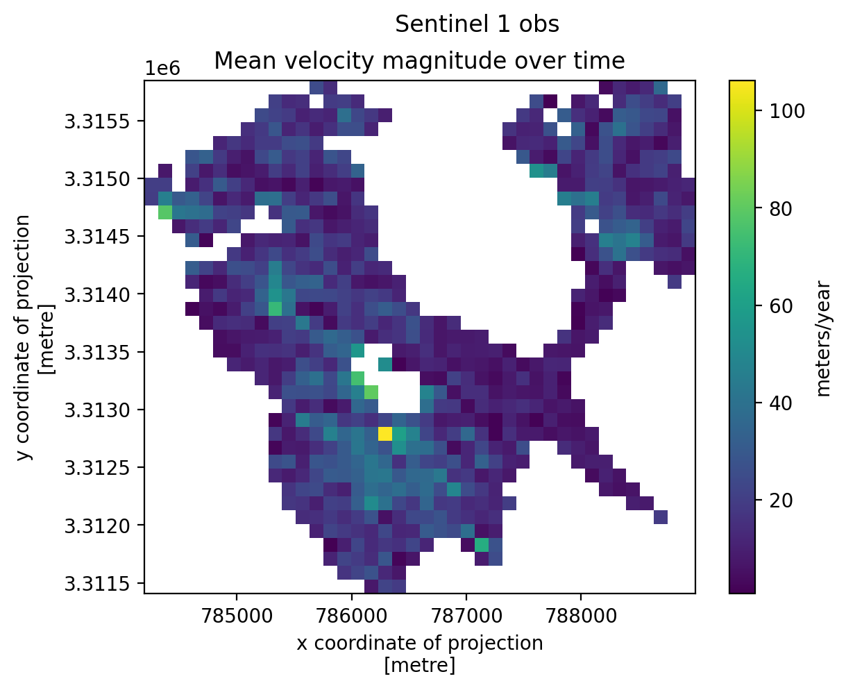
s2_condition = sample_glacier_raster.satellite_img1.isin(['2A','2B'])
s2_subset = sample_glacier_raster.sel(mid_date=s2_condition)
s2_subset
<xarray.Dataset> Size: 181MB
Dimensions: (mid_date: 2342, y: 37, x: 40)
Coordinates:
* mid_date (mid_date) datetime64[ns] 19kB 2018-04-14T04:...
* x (x) float64 320B 7.843e+05 ... 7.889e+05
* y (y) float64 296B 3.316e+06 ... 3.311e+06
spatial_ref int64 8B 0
mapping int64 8B 0
Data variables: (12/59)
M11 (mid_date, y, x) float32 14MB nan nan ... nan
M11_dr_to_vr_factor (mid_date) float32 9kB nan nan nan ... nan nan
M12 (mid_date, y, x) float32 14MB nan nan ... nan
M12_dr_to_vr_factor (mid_date) float32 9kB nan nan nan ... nan nan
acquisition_date_img1 (mid_date) datetime64[ns] 19kB 2017-12-20T04:...
acquisition_date_img2 (mid_date) datetime64[ns] 19kB 2018-08-07T04:...
... ...
vy_error_modeled (mid_date) float32 9kB 40.5 28.6 ... 60.0 30.0
vy_error_slow (mid_date) float32 9kB 8.0 1.7 1.2 ... 12.9 3.6
vy_error_stationary (mid_date) float32 9kB 8.0 1.7 1.2 ... 12.9 3.6
vy_stable_shift (mid_date) float32 9kB 8.9 -4.9 -0.7 ... 8.4 2.9
vy_stable_shift_slow (mid_date) float32 9kB 8.9 -4.9 -0.7 ... 8.4 2.9
vy_stable_shift_stationary (mid_date) float32 9kB 8.9 -4.9 -0.7 ... 8.4 2.9
Attributes: (12/19)
Conventions: CF-1.8
GDAL_AREA_OR_POINT: Area
author: ITS_LIVE, a NASA MEaSUREs project (its-live.j...
autoRIFT_parameter_file: http://its-live-data.s3.amazonaws.com/autorif...
datacube_software_version: 1.0
date_created: 25-Sep-2023 22:00:23
... ...
s3: s3://its-live-data/datacubes/v2/N30E090/ITS_L...
skipped_granules: s3://its-live-data/datacubes/v2/N30E090/ITS_L...
time_standard_img1: UTC
time_standard_img2: UTC
title: ITS_LIVE datacube of image pair velocities
url: https://its-live-data.s3.amazonaws.com/datacu...- mid_date: 2342
- y: 37
- x: 40
- mid_date(mid_date)datetime64[ns]2018-04-14T04:18:49.171219968 .....
- description :
- midpoint of image 1 and image 2 acquisition date and time with granule's centroid longitude and latitude as microseconds
- standard_name :
- image_pair_center_date_with_time_separation
array(['2018-04-14T04:18:49.171219968', '2017-02-10T16:15:50.660901120', '2019-03-15T04:15:44.180925952', ..., '2019-03-30T04:15:51.181000960', '2019-08-29T16:18:15.190612992', '2018-04-24T04:18:14.171119872'], shape=(2342,), dtype='datetime64[ns]') - x(x)float647.843e+05 7.844e+05 ... 7.889e+05
- description :
- x coordinate of projection
- standard_name :
- projection_x_coordinate
- axis :
- X
- long_name :
- x coordinate of projection
- units :
- metre
array([784252.5, 784372.5, 784492.5, 784612.5, 784732.5, 784852.5, 784972.5, 785092.5, 785212.5, 785332.5, 785452.5, 785572.5, 785692.5, 785812.5, 785932.5, 786052.5, 786172.5, 786292.5, 786412.5, 786532.5, 786652.5, 786772.5, 786892.5, 787012.5, 787132.5, 787252.5, 787372.5, 787492.5, 787612.5, 787732.5, 787852.5, 787972.5, 788092.5, 788212.5, 788332.5, 788452.5, 788572.5, 788692.5, 788812.5, 788932.5]) - y(y)float643.316e+06 3.316e+06 ... 3.311e+06
- description :
- y coordinate of projection
- standard_name :
- projection_y_coordinate
- axis :
- Y
- long_name :
- y coordinate of projection
- units :
- metre
array([3315787.5, 3315667.5, 3315547.5, 3315427.5, 3315307.5, 3315187.5, 3315067.5, 3314947.5, 3314827.5, 3314707.5, 3314587.5, 3314467.5, 3314347.5, 3314227.5, 3314107.5, 3313987.5, 3313867.5, 3313747.5, 3313627.5, 3313507.5, 3313387.5, 3313267.5, 3313147.5, 3313027.5, 3312907.5, 3312787.5, 3312667.5, 3312547.5, 3312427.5, 3312307.5, 3312187.5, 3312067.5, 3311947.5, 3311827.5, 3311707.5, 3311587.5, 3311467.5]) - spatial_ref()int640
- GeoTransform :
- 784192.5 120.0 0.0 3315847.5 0.0 -120.0
array(0)
- mapping()int640
- crs_wkt :
- PROJCS["WGS 84 / UTM zone 46N",GEOGCS["WGS 84",DATUM["WGS_1984",SPHEROID["WGS 84",6378137,298.257223563,AUTHORITY["EPSG","7030"]],AUTHORITY["EPSG","6326"]],PRIMEM["Greenwich",0,AUTHORITY["EPSG","8901"]],UNIT["degree",0.0174532925199433,AUTHORITY["EPSG","9122"]],AUTHORITY["EPSG","4326"]],PROJECTION["Transverse_Mercator"],PARAMETER["latitude_of_origin",0],PARAMETER["central_meridian",93],PARAMETER["scale_factor",0.9996],PARAMETER["false_easting",500000],PARAMETER["false_northing",0],UNIT["metre",1,AUTHORITY["EPSG","9001"]],AXIS["Easting",EAST],AXIS["Northing",NORTH],AUTHORITY["EPSG","32646"]]
- semi_major_axis :
- 6378137.0
- semi_minor_axis :
- 6356752.314245179
- inverse_flattening :
- 298.257223563
- reference_ellipsoid_name :
- WGS 84
- longitude_of_prime_meridian :
- 0.0
- prime_meridian_name :
- Greenwich
- geographic_crs_name :
- WGS 84
- horizontal_datum_name :
- World Geodetic System 1984
- projected_crs_name :
- WGS 84 / UTM zone 46N
- grid_mapping_name :
- transverse_mercator
- latitude_of_projection_origin :
- 0.0
- longitude_of_central_meridian :
- 93.0
- false_easting :
- 500000.0
- false_northing :
- 0.0
- scale_factor_at_central_meridian :
- 0.9996
- spatial_ref :
- PROJCS["WGS 84 / UTM zone 46N",GEOGCS["WGS 84",DATUM["WGS_1984",SPHEROID["WGS 84",6378137,298.257223563,AUTHORITY["EPSG","7030"]],AUTHORITY["EPSG","6326"]],PRIMEM["Greenwich",0,AUTHORITY["EPSG","8901"]],UNIT["degree",0.0174532925199433,AUTHORITY["EPSG","9122"]],AUTHORITY["EPSG","4326"]],PROJECTION["Transverse_Mercator"],PARAMETER["latitude_of_origin",0],PARAMETER["central_meridian",93],PARAMETER["scale_factor",0.9996],PARAMETER["false_easting",500000],PARAMETER["false_northing",0],UNIT["metre",1,AUTHORITY["EPSG","9001"]],AXIS["Easting",EAST],AXIS["Northing",NORTH],AUTHORITY["EPSG","32646"]]
- GeoTransform :
- 784192.5 120.0 0.0 3315847.5 0.0 -120.0
array(0)
- M11(mid_date, y, x)float32nan nan nan nan ... nan nan nan nan
- description :
- conversion matrix element (1st row, 1st column) that can be multiplied with vx to give range pixel displacement dr (see Eq. A18 in https://www.mdpi.com/2072-4292/13/4/749)
- standard_name :
- conversion_matrix_element_11
- units :
- pixel/(meter/year)
array([[[nan, nan, nan, ..., nan, nan, nan], [nan, nan, nan, ..., nan, nan, nan], [nan, nan, nan, ..., nan, nan, nan], ..., [nan, nan, nan, ..., nan, nan, nan], [nan, nan, nan, ..., nan, nan, nan], [nan, nan, nan, ..., nan, nan, nan]], [[nan, nan, nan, ..., nan, nan, nan], [nan, nan, nan, ..., nan, nan, nan], [nan, nan, nan, ..., nan, nan, nan], ..., [nan, nan, nan, ..., nan, nan, nan], [nan, nan, nan, ..., nan, nan, nan], [nan, nan, nan, ..., nan, nan, nan]], [[nan, nan, nan, ..., nan, nan, nan], [nan, nan, nan, ..., nan, nan, nan], [nan, nan, nan, ..., nan, nan, nan], ..., ... [nan, nan, nan, ..., nan, nan, nan], [nan, nan, nan, ..., nan, nan, nan], [nan, nan, nan, ..., nan, nan, nan]], [[nan, nan, nan, ..., nan, nan, nan], [nan, nan, nan, ..., nan, nan, nan], [nan, nan, nan, ..., nan, nan, nan], ..., [nan, nan, nan, ..., nan, nan, nan], [nan, nan, nan, ..., nan, nan, nan], [nan, nan, nan, ..., nan, nan, nan]], [[nan, nan, nan, ..., nan, nan, nan], [nan, nan, nan, ..., nan, nan, nan], [nan, nan, nan, ..., nan, nan, nan], ..., [nan, nan, nan, ..., nan, nan, nan], [nan, nan, nan, ..., nan, nan, nan], [nan, nan, nan, ..., nan, nan, nan]]], shape=(2342, 37, 40), dtype=float32) - M11_dr_to_vr_factor(mid_date)float32nan nan nan nan ... nan nan nan nan
- description :
- multiplicative factor that converts slant range pixel displacement dr to slant range velocity vr
- standard_name :
- M11_dr_to_vr_factor
- units :
- meter/(year*pixel)
array([nan, nan, nan, ..., nan, nan, nan], shape=(2342,), dtype=float32)
- M12(mid_date, y, x)float32nan nan nan nan ... nan nan nan nan
- description :
- conversion matrix element (1st row, 2nd column) that can be multiplied with vy to give range pixel displacement dr (see Eq. A18 in https://www.mdpi.com/2072-4292/13/4/749)
- standard_name :
- conversion_matrix_element_12
- units :
- pixel/(meter/year)
array([[[nan, nan, nan, ..., nan, nan, nan], [nan, nan, nan, ..., nan, nan, nan], [nan, nan, nan, ..., nan, nan, nan], ..., [nan, nan, nan, ..., nan, nan, nan], [nan, nan, nan, ..., nan, nan, nan], [nan, nan, nan, ..., nan, nan, nan]], [[nan, nan, nan, ..., nan, nan, nan], [nan, nan, nan, ..., nan, nan, nan], [nan, nan, nan, ..., nan, nan, nan], ..., [nan, nan, nan, ..., nan, nan, nan], [nan, nan, nan, ..., nan, nan, nan], [nan, nan, nan, ..., nan, nan, nan]], [[nan, nan, nan, ..., nan, nan, nan], [nan, nan, nan, ..., nan, nan, nan], [nan, nan, nan, ..., nan, nan, nan], ..., ... [nan, nan, nan, ..., nan, nan, nan], [nan, nan, nan, ..., nan, nan, nan], [nan, nan, nan, ..., nan, nan, nan]], [[nan, nan, nan, ..., nan, nan, nan], [nan, nan, nan, ..., nan, nan, nan], [nan, nan, nan, ..., nan, nan, nan], ..., [nan, nan, nan, ..., nan, nan, nan], [nan, nan, nan, ..., nan, nan, nan], [nan, nan, nan, ..., nan, nan, nan]], [[nan, nan, nan, ..., nan, nan, nan], [nan, nan, nan, ..., nan, nan, nan], [nan, nan, nan, ..., nan, nan, nan], ..., [nan, nan, nan, ..., nan, nan, nan], [nan, nan, nan, ..., nan, nan, nan], [nan, nan, nan, ..., nan, nan, nan]]], shape=(2342, 37, 40), dtype=float32) - M12_dr_to_vr_factor(mid_date)float32nan nan nan nan ... nan nan nan nan
- description :
- multiplicative factor that converts slant range pixel displacement dr to slant range velocity vr
- standard_name :
- M12_dr_to_vr_factor
- units :
- meter/(year*pixel)
array([nan, nan, nan, ..., nan, nan, nan], shape=(2342,), dtype=float32)
- acquisition_date_img1(mid_date)datetime64[ns]2017-12-20T04:21:49 ... 2017-11-...
- description :
- acquisition date and time of image 1
- standard_name :
- image1_acquition_date
array(['2017-12-20T04:21:49.000000000', '2016-09-01T04:15:52.000000000', '2018-09-26T04:15:39.000000000', ..., '2018-10-01T04:15:51.000000000', '2019-06-13T04:15:58.999999744', '2017-11-20T04:20:49.000000000'], shape=(2342,), dtype='datetime64[ns]') - acquisition_date_img2(mid_date)datetime64[ns]2018-08-07T04:15:49 ... 2018-09-...
- description :
- acquisition date and time of image 2
- standard_name :
- image2_acquition_date
array(['2018-08-07T04:15:49.000000000', '2017-07-23T04:15:49.000000000', '2019-09-01T04:15:49.000000000', ..., '2019-09-26T04:15:51.000000000', '2019-11-15T04:20:31.000000000', '2018-09-26T04:15:39.000000000'], shape=(2342,), dtype='datetime64[ns]') - autoRIFT_software_version(mid_date)object'1.5.0' '1.5.0' ... '1.5.0' '1.5.0'
- description :
- version of autoRIFT software
- standard_name :
- autoRIFT_software_version
array(['1.5.0', '1.5.0', '1.5.0', ..., '1.5.0', '1.5.0', '1.5.0'], shape=(2342,), dtype=object) - chip_size_height(mid_date, y, x)float32nan nan nan nan ... nan nan nan nan
- chip_size_coordinates :
- Optical data: chip_size_coordinates = 'image projection geometry: width = x, height = y'. Radar data: chip_size_coordinates = 'radar geometry: width = range, height = azimuth'
- description :
- height of search template (chip)
- standard_name :
- chip_size_height
- units :
- m
- y_pixel_size :
- 10.0
array([[[nan, nan, nan, ..., nan, nan, nan], [nan, nan, nan, ..., nan, nan, nan], [nan, nan, nan, ..., nan, nan, nan], ..., [nan, nan, nan, ..., nan, nan, nan], [nan, nan, nan, ..., nan, nan, nan], [nan, nan, nan, ..., nan, nan, nan]], [[nan, nan, nan, ..., nan, nan, nan], [nan, nan, nan, ..., nan, nan, nan], [nan, nan, nan, ..., nan, nan, nan], ..., [nan, nan, nan, ..., nan, nan, nan], [nan, nan, nan, ..., nan, nan, nan], [nan, nan, nan, ..., nan, nan, nan]], [[nan, nan, nan, ..., nan, nan, nan], [nan, nan, nan, ..., nan, nan, nan], [nan, nan, nan, ..., nan, nan, nan], ..., ... [nan, nan, nan, ..., nan, nan, nan], [nan, nan, nan, ..., nan, nan, nan], [nan, nan, nan, ..., nan, nan, nan]], [[nan, nan, nan, ..., nan, nan, nan], [nan, nan, nan, ..., nan, nan, nan], [nan, nan, nan, ..., nan, nan, nan], ..., [nan, nan, nan, ..., nan, nan, nan], [nan, nan, nan, ..., nan, nan, nan], [nan, nan, nan, ..., nan, nan, nan]], [[nan, nan, nan, ..., nan, nan, nan], [nan, nan, nan, ..., nan, nan, nan], [nan, nan, nan, ..., nan, nan, nan], ..., [nan, nan, nan, ..., nan, nan, nan], [nan, nan, nan, ..., nan, nan, nan], [nan, nan, nan, ..., nan, nan, nan]]], shape=(2342, 37, 40), dtype=float32) - chip_size_width(mid_date, y, x)float32nan nan nan nan ... nan nan nan nan
- chip_size_coordinates :
- Optical data: chip_size_coordinates = 'image projection geometry: width = x, height = y'. Radar data: chip_size_coordinates = 'radar geometry: width = range, height = azimuth'
- description :
- width of search template (chip)
- standard_name :
- chip_size_width
- units :
- m
- x_pixel_size :
- 10.0
array([[[nan, nan, nan, ..., nan, nan, nan], [nan, nan, nan, ..., nan, nan, nan], [nan, nan, nan, ..., nan, nan, nan], ..., [nan, nan, nan, ..., nan, nan, nan], [nan, nan, nan, ..., nan, nan, nan], [nan, nan, nan, ..., nan, nan, nan]], [[nan, nan, nan, ..., nan, nan, nan], [nan, nan, nan, ..., nan, nan, nan], [nan, nan, nan, ..., nan, nan, nan], ..., [nan, nan, nan, ..., nan, nan, nan], [nan, nan, nan, ..., nan, nan, nan], [nan, nan, nan, ..., nan, nan, nan]], [[nan, nan, nan, ..., nan, nan, nan], [nan, nan, nan, ..., nan, nan, nan], [nan, nan, nan, ..., nan, nan, nan], ..., ... [nan, nan, nan, ..., nan, nan, nan], [nan, nan, nan, ..., nan, nan, nan], [nan, nan, nan, ..., nan, nan, nan]], [[nan, nan, nan, ..., nan, nan, nan], [nan, nan, nan, ..., nan, nan, nan], [nan, nan, nan, ..., nan, nan, nan], ..., [nan, nan, nan, ..., nan, nan, nan], [nan, nan, nan, ..., nan, nan, nan], [nan, nan, nan, ..., nan, nan, nan]], [[nan, nan, nan, ..., nan, nan, nan], [nan, nan, nan, ..., nan, nan, nan], [nan, nan, nan, ..., nan, nan, nan], ..., [nan, nan, nan, ..., nan, nan, nan], [nan, nan, nan, ..., nan, nan, nan], [nan, nan, nan, ..., nan, nan, nan]]], shape=(2342, 37, 40), dtype=float32) - date_center(mid_date)datetime64[ns]2018-04-14T04:18:49 ... 2018-04-...
- description :
- midpoint of image 1 and image 2 acquisition date
- standard_name :
- image_pair_center_date
array(['2018-04-14T04:18:49.000000000', '2017-02-10T16:15:50.500000000', '2019-03-15T04:15:44.000000000', ..., '2019-03-30T04:15:51.000000000', '2019-08-29T16:18:15.000000000', '2018-04-24T04:18:14.000000000'], shape=(2342,), dtype='datetime64[ns]') - date_dt(mid_date)timedelta64[ns]229 days 23:54:00.087890621 ... ...
- description :
- time separation between acquisition of image 1 and image 2
- standard_name :
- image_pair_time_separation
array([19871640087890621, 28079997363281252, 29376010546875000, ..., 31104000000000000, 13392271582031252, 26783688867187495], shape=(2342,), dtype='timedelta64[ns]') - floatingice(y, x, mid_date)float32nan nan nan nan ... nan nan nan nan
- description :
- floating ice mask, 0 = non-floating-ice, 1 = floating-ice
- flag_meanings :
- non-ice ice
- flag_values :
- [0, 1]
- standard_name :
- floating ice mask
- url :
- https://its-live-data.s3.amazonaws.com/autorift_parameters/v001/N46_0120m_floatingice.tif
array([[[nan, nan, nan, ..., nan, nan, nan], [nan, nan, nan, ..., nan, nan, nan], [nan, nan, nan, ..., nan, nan, nan], ..., [ 0., 0., 0., ..., 0., 0., 0.], [nan, nan, nan, ..., nan, nan, nan], [nan, nan, nan, ..., nan, nan, nan]], [[nan, nan, nan, ..., nan, nan, nan], [nan, nan, nan, ..., nan, nan, nan], [nan, nan, nan, ..., nan, nan, nan], ..., [ 0., 0., 0., ..., 0., 0., 0.], [ 0., 0., 0., ..., 0., 0., 0.], [nan, nan, nan, ..., nan, nan, nan]], [[nan, nan, nan, ..., nan, nan, nan], [nan, nan, nan, ..., nan, nan, nan], [nan, nan, nan, ..., nan, nan, nan], ..., ... [nan, nan, nan, ..., nan, nan, nan], [nan, nan, nan, ..., nan, nan, nan], [nan, nan, nan, ..., nan, nan, nan]], [[nan, nan, nan, ..., nan, nan, nan], [nan, nan, nan, ..., nan, nan, nan], [nan, nan, nan, ..., nan, nan, nan], ..., [nan, nan, nan, ..., nan, nan, nan], [nan, nan, nan, ..., nan, nan, nan], [nan, nan, nan, ..., nan, nan, nan]], [[nan, nan, nan, ..., nan, nan, nan], [nan, nan, nan, ..., nan, nan, nan], [nan, nan, nan, ..., nan, nan, nan], ..., [nan, nan, nan, ..., nan, nan, nan], [nan, nan, nan, ..., nan, nan, nan], [nan, nan, nan, ..., nan, nan, nan]]], shape=(37, 40, 2342), dtype=float32) - granule_url(mid_date)object'https://its-live-data.s3.amazon...
- description :
- original granule URL
- standard_name :
- granule_url
array(['https://its-live-data.s3.amazonaws.com/velocity_image_pair/sentinel2/v02/N30E090/S2B_MSIL1C_20171220T042149_N0206_R090_T46RGU_20171220T071238_X_S2B_MSIL1C_20180807T041549_N0206_R090_T46RGU_20180807T080037_G0120V02_P017.nc', 'https://its-live-data.s3.amazonaws.com/velocity_image_pair/sentinel2/v02/N30E090/S2A_MSIL1C_20160901T041552_N0204_R090_T46RGV_20160901T042146_X_S2B_MSIL1C_20170723T041549_N0205_R090_T46RGV_20170723T042211_G0120V02_P011.nc', 'https://its-live-data.s3.amazonaws.com/velocity_image_pair/sentinel2/v02/N30E090/S2B_MSIL1C_20180926T041539_N0206_R090_T46RFV_20180926T085405_X_S2B_MSIL1C_20190901T041549_N0208_R090_T46RFV_20190901T084626_G0120V02_P051.nc', ..., 'https://its-live-data.s3.amazonaws.com/velocity_image_pair/sentinel2/v02/N30E090/S2A_MSIL1C_20181001T041551_N0206_R090_T46RFV_20181001T072036_X_S2A_MSIL1C_20190926T041551_N0208_R090_T46RFV_20190926T071222_G0120V02_P056.nc', 'https://its-live-data.s3.amazonaws.com/velocity_image_pair/sentinel2/v02/N30E090/S2B_MSIL1C_20190613T041559_N0207_R090_T46RFV_20190613T071505_X_S2A_MSIL1C_20191115T042031_N0208_R090_T46RFV_20191115T072359_G0120V02_P056.nc', 'https://its-live-data.s3.amazonaws.com/velocity_image_pair/sentinel2/v02/N30E090/S2B_MSIL1C_20171120T042049_N0206_R090_T46RGV_20171121T055049_X_S2B_MSIL1C_20180926T041539_N0206_R090_T46RGV_20180926T085405_G0120V02_P057.nc'], shape=(2342,), dtype=object) - interp_mask(mid_date, y, x)float32nan nan nan nan ... nan nan nan nan
- description :
- light interpolation mask
- flag_meanings :
- measured interpolated
- flag_values :
- [0, 1]
- standard_name :
- interpolated_value_mask
array([[[nan, nan, nan, ..., nan, nan, nan], [nan, nan, nan, ..., nan, nan, nan], [nan, nan, nan, ..., nan, nan, nan], ..., [nan, nan, nan, ..., nan, nan, nan], [nan, nan, nan, ..., nan, nan, nan], [nan, nan, nan, ..., nan, nan, nan]], [[nan, nan, nan, ..., nan, nan, nan], [nan, nan, nan, ..., nan, nan, nan], [nan, nan, nan, ..., nan, nan, nan], ..., [nan, nan, nan, ..., nan, nan, nan], [nan, nan, nan, ..., nan, nan, nan], [nan, nan, nan, ..., nan, nan, nan]], [[nan, nan, nan, ..., nan, nan, nan], [nan, nan, nan, ..., nan, nan, nan], [nan, nan, nan, ..., nan, nan, nan], ..., ... [nan, nan, nan, ..., nan, nan, nan], [nan, nan, nan, ..., nan, nan, nan], [nan, nan, nan, ..., nan, nan, nan]], [[nan, nan, nan, ..., nan, nan, nan], [nan, nan, nan, ..., nan, nan, nan], [nan, nan, nan, ..., nan, nan, nan], ..., [nan, nan, nan, ..., nan, nan, nan], [nan, nan, nan, ..., nan, nan, nan], [nan, nan, nan, ..., nan, nan, nan]], [[nan, nan, nan, ..., nan, nan, nan], [nan, nan, nan, ..., nan, nan, nan], [nan, nan, nan, ..., nan, nan, nan], ..., [nan, nan, nan, ..., nan, nan, nan], [nan, nan, nan, ..., nan, nan, nan], [nan, nan, nan, ..., nan, nan, nan]]], shape=(2342, 37, 40), dtype=float32) - landice(y, x, mid_date)float32nan nan nan nan ... nan nan nan nan
- description :
- land ice mask, 0 = non-land-ice, 1 = land-ice
- flag_meanings :
- non-ice ice
- flag_values :
- [0, 1]
- standard_name :
- land ice mask
- url :
- https://its-live-data.s3.amazonaws.com/autorift_parameters/v001/N46_0120m_landice.tif
array([[[nan, nan, nan, ..., nan, nan, nan], [nan, nan, nan, ..., nan, nan, nan], [nan, nan, nan, ..., nan, nan, nan], ..., [ 1., 1., 1., ..., 1., 1., 1.], [nan, nan, nan, ..., nan, nan, nan], [nan, nan, nan, ..., nan, nan, nan]], [[nan, nan, nan, ..., nan, nan, nan], [nan, nan, nan, ..., nan, nan, nan], [nan, nan, nan, ..., nan, nan, nan], ..., [ 1., 1., 1., ..., 1., 1., 1.], [ 1., 1., 1., ..., 1., 1., 1.], [nan, nan, nan, ..., nan, nan, nan]], [[nan, nan, nan, ..., nan, nan, nan], [nan, nan, nan, ..., nan, nan, nan], [nan, nan, nan, ..., nan, nan, nan], ..., ... [nan, nan, nan, ..., nan, nan, nan], [nan, nan, nan, ..., nan, nan, nan], [nan, nan, nan, ..., nan, nan, nan]], [[nan, nan, nan, ..., nan, nan, nan], [nan, nan, nan, ..., nan, nan, nan], [nan, nan, nan, ..., nan, nan, nan], ..., [nan, nan, nan, ..., nan, nan, nan], [nan, nan, nan, ..., nan, nan, nan], [nan, nan, nan, ..., nan, nan, nan]], [[nan, nan, nan, ..., nan, nan, nan], [nan, nan, nan, ..., nan, nan, nan], [nan, nan, nan, ..., nan, nan, nan], ..., [nan, nan, nan, ..., nan, nan, nan], [nan, nan, nan, ..., nan, nan, nan], [nan, nan, nan, ..., nan, nan, nan]]], shape=(37, 40, 2342), dtype=float32) - mission_img1(mid_date)object'S' 'S' 'S' 'S' ... 'S' 'S' 'S' 'S'
- description :
- id of the mission that acquired image 1
- standard_name :
- image1_mission
array(['S', 'S', 'S', ..., 'S', 'S', 'S'], shape=(2342,), dtype=object)
- mission_img2(mid_date)object'S' 'S' 'S' 'S' ... 'S' 'S' 'S' 'S'
- description :
- id of the mission that acquired image 2
- standard_name :
- image2_mission
array(['S', 'S', 'S', ..., 'S', 'S', 'S'], shape=(2342,), dtype=object)
- roi_valid_percentage(mid_date)float3217.8 11.1 51.2 ... 56.0 56.9 57.6
- description :
- percentage of pixels with a valid velocity estimate determined for the intersection of the full image pair footprint and the region of interest (roi) that defines where autoRIFT tried to estimate a velocity
- standard_name :
- region_of_interest_valid_pixel_percentage
array([17.8, 11.1, 51.2, ..., 56. , 56.9, 57.6], shape=(2342,), dtype=float32) - satellite_img1(mid_date)object'2B' '2A' '2B' ... '2A' '2B' '2B'
- description :
- id of the satellite that acquired image 1
- standard_name :
- image1_satellite
array(['2B', '2A', '2B', ..., '2A', '2B', '2B'], shape=(2342,), dtype=object) - satellite_img2(mid_date)object'2B' '2B' '2B' ... '2A' '2A' '2B'
- description :
- id of the satellite that acquired image 2
- standard_name :
- image2_satellite
array(['2B', '2B', '2B', ..., '2A', '2A', '2B'], shape=(2342,), dtype=object) - sensor_img1(mid_date)object'MSI' 'MSI' 'MSI' ... 'MSI' 'MSI'
- description :
- id of the sensor that acquired image 1
- standard_name :
- image1_sensor
array(['MSI', 'MSI', 'MSI', ..., 'MSI', 'MSI', 'MSI'], shape=(2342,), dtype=object) - sensor_img2(mid_date)object'MSI' 'MSI' 'MSI' ... 'MSI' 'MSI'
- description :
- id of the sensor that acquired image 2
- standard_name :
- image2_sensor
array(['MSI', 'MSI', 'MSI', ..., 'MSI', 'MSI', 'MSI'], shape=(2342,), dtype=object) - stable_count_slow(mid_date)float328.941e+03 3.531e+04 ... 5.165e+04
- description :
- number of valid pixels over slowest 25% of ice
- standard_name :
- stable_count_slow
- units :
- count
array([ 8941., 35311., 35175., ..., 4723., 3917., 51652.], shape=(2342,), dtype=float32) - stable_count_stationary(mid_date)float328.446e+03 3.529e+04 ... 5.152e+04
- description :
- number of valid pixels over stationary or slow-flowing surfaces
- standard_name :
- stable_count_stationary
- units :
- count
array([ 8446., 35290., 34638., ..., 3589., 2400., 51519.], shape=(2342,), dtype=float32) - stable_shift_flag(mid_date)float321.0 1.0 1.0 1.0 ... 1.0 1.0 1.0 1.0
- description :
- flag for applying velocity bias correction: 0 = no correction; 1 = correction from overlapping stable surface mask (stationary or slow-flowing surfaces with velocity < 15 m/yr)(top priority); 2 = correction from slowest 25% of overlapping velocities (second priority)
- standard_name :
- stable_shift_flag
array([1., 1., 1., ..., 1., 1., 1.], shape=(2342,), dtype=float32)
- v(mid_date, y, x)float32nan nan nan nan ... nan nan nan nan
- description :
- velocity magnitude
- standard_name :
- land_ice_surface_velocity
- units :
- meter/year
array([[[nan, nan, nan, ..., nan, nan, nan], [nan, nan, nan, ..., nan, nan, nan], [nan, nan, nan, ..., nan, nan, nan], ..., [nan, nan, nan, ..., nan, nan, nan], [nan, nan, nan, ..., nan, nan, nan], [nan, nan, nan, ..., nan, nan, nan]], [[nan, nan, nan, ..., nan, nan, nan], [nan, nan, nan, ..., nan, nan, nan], [nan, nan, nan, ..., nan, nan, nan], ..., [nan, nan, nan, ..., nan, nan, nan], [nan, nan, nan, ..., nan, nan, nan], [nan, nan, nan, ..., nan, nan, nan]], [[nan, nan, nan, ..., nan, nan, nan], [nan, nan, nan, ..., nan, nan, nan], [nan, nan, nan, ..., nan, nan, nan], ..., ... [nan, nan, nan, ..., nan, nan, nan], [nan, nan, nan, ..., nan, nan, nan], [nan, nan, nan, ..., nan, nan, nan]], [[nan, nan, nan, ..., nan, nan, nan], [nan, nan, nan, ..., nan, nan, nan], [nan, nan, nan, ..., nan, nan, nan], ..., [nan, nan, nan, ..., nan, nan, nan], [nan, nan, nan, ..., nan, nan, nan], [nan, nan, nan, ..., nan, nan, nan]], [[nan, nan, nan, ..., nan, nan, nan], [nan, nan, nan, ..., nan, nan, nan], [nan, nan, nan, ..., nan, nan, nan], ..., [nan, nan, nan, ..., nan, nan, nan], [nan, nan, nan, ..., nan, nan, nan], [nan, nan, nan, ..., nan, nan, nan]]], shape=(2342, 37, 40), dtype=float32) - v_error(mid_date, y, x)float32nan nan nan nan ... nan nan nan nan
- description :
- velocity magnitude error
- standard_name :
- velocity_error
- units :
- meter/year
array([[[nan, nan, nan, ..., nan, nan, nan], [nan, nan, nan, ..., nan, nan, nan], [nan, nan, nan, ..., nan, nan, nan], ..., [nan, nan, nan, ..., nan, nan, nan], [nan, nan, nan, ..., nan, nan, nan], [nan, nan, nan, ..., nan, nan, nan]], [[nan, nan, nan, ..., nan, nan, nan], [nan, nan, nan, ..., nan, nan, nan], [nan, nan, nan, ..., nan, nan, nan], ..., [nan, nan, nan, ..., nan, nan, nan], [nan, nan, nan, ..., nan, nan, nan], [nan, nan, nan, ..., nan, nan, nan]], [[nan, nan, nan, ..., nan, nan, nan], [nan, nan, nan, ..., nan, nan, nan], [nan, nan, nan, ..., nan, nan, nan], ..., ... [nan, nan, nan, ..., nan, nan, nan], [nan, nan, nan, ..., nan, nan, nan], [nan, nan, nan, ..., nan, nan, nan]], [[nan, nan, nan, ..., nan, nan, nan], [nan, nan, nan, ..., nan, nan, nan], [nan, nan, nan, ..., nan, nan, nan], ..., [nan, nan, nan, ..., nan, nan, nan], [nan, nan, nan, ..., nan, nan, nan], [nan, nan, nan, ..., nan, nan, nan]], [[nan, nan, nan, ..., nan, nan, nan], [nan, nan, nan, ..., nan, nan, nan], [nan, nan, nan, ..., nan, nan, nan], ..., [nan, nan, nan, ..., nan, nan, nan], [nan, nan, nan, ..., nan, nan, nan], [nan, nan, nan, ..., nan, nan, nan]]], shape=(2342, 37, 40), dtype=float32) - va(mid_date, y, x)float32nan nan nan nan ... nan nan nan nan
- description :
- velocity in radar azimuth direction
array([[[nan, nan, nan, ..., nan, nan, nan], [nan, nan, nan, ..., nan, nan, nan], [nan, nan, nan, ..., nan, nan, nan], ..., [nan, nan, nan, ..., nan, nan, nan], [nan, nan, nan, ..., nan, nan, nan], [nan, nan, nan, ..., nan, nan, nan]], [[nan, nan, nan, ..., nan, nan, nan], [nan, nan, nan, ..., nan, nan, nan], [nan, nan, nan, ..., nan, nan, nan], ..., [nan, nan, nan, ..., nan, nan, nan], [nan, nan, nan, ..., nan, nan, nan], [nan, nan, nan, ..., nan, nan, nan]], [[nan, nan, nan, ..., nan, nan, nan], [nan, nan, nan, ..., nan, nan, nan], [nan, nan, nan, ..., nan, nan, nan], ..., ... [nan, nan, nan, ..., nan, nan, nan], [nan, nan, nan, ..., nan, nan, nan], [nan, nan, nan, ..., nan, nan, nan]], [[nan, nan, nan, ..., nan, nan, nan], [nan, nan, nan, ..., nan, nan, nan], [nan, nan, nan, ..., nan, nan, nan], ..., [nan, nan, nan, ..., nan, nan, nan], [nan, nan, nan, ..., nan, nan, nan], [nan, nan, nan, ..., nan, nan, nan]], [[nan, nan, nan, ..., nan, nan, nan], [nan, nan, nan, ..., nan, nan, nan], [nan, nan, nan, ..., nan, nan, nan], ..., [nan, nan, nan, ..., nan, nan, nan], [nan, nan, nan, ..., nan, nan, nan], [nan, nan, nan, ..., nan, nan, nan]]], shape=(2342, 37, 40), dtype=float32) - va_error(mid_date)float32nan nan nan nan ... nan nan nan nan
- description :
- error for velocity in radar azimuth direction
- standard_name :
- va_error
- units :
- meter/year
array([nan, nan, nan, ..., nan, nan, nan], shape=(2342,), dtype=float32)
- va_error_modeled(mid_date)float32nan nan nan nan ... nan nan nan nan
- description :
- 1-sigma error calculated using a modeled error-dt relationship
- standard_name :
- va_error_modeled
- units :
- meter/year
array([nan, nan, nan, ..., nan, nan, nan], shape=(2342,), dtype=float32)
- va_error_slow(mid_date)float32nan nan nan nan ... nan nan nan nan
- description :
- RMSE over slowest 25% of retrieved velocities
- standard_name :
- va_error_slow
- units :
- meter/year
array([nan, nan, nan, ..., nan, nan, nan], shape=(2342,), dtype=float32)
- va_error_stationary(mid_date)float32nan nan nan nan ... nan nan nan nan
- description :
- RMSE over stable surfaces, stationary or slow-flowing surfaces with velocity < 15 m/yr identified from an external mask
- standard_name :
- va_error_stationary
- units :
- meter/year
array([nan, nan, nan, ..., nan, nan, nan], shape=(2342,), dtype=float32)
- va_stable_shift(mid_date)float32nan nan nan nan ... nan nan nan nan
- description :
- applied va shift calibrated using pixels over stable or slow surfaces
- standard_name :
- va_stable_shift
- units :
- meter/year
array([nan, nan, nan, ..., nan, nan, nan], shape=(2342,), dtype=float32)
- va_stable_shift_slow(mid_date)float32nan nan nan nan ... nan nan nan nan
- description :
- va shift calibrated using valid pixels over slowest 25% of retrieved velocities
- standard_name :
- va_stable_shift_slow
- units :
- meter/year
array([nan, nan, nan, ..., nan, nan, nan], shape=(2342,), dtype=float32)
- va_stable_shift_stationary(mid_date)float32nan nan nan nan ... nan nan nan nan
- description :
- va shift calibrated using valid pixels over stable surfaces, stationary or slow-flowing surfaces with velocity < 15 m/yr identified from an external mask
- standard_name :
- va_stable_shift_stationary
- units :
- meter/year
array([nan, nan, nan, ..., nan, nan, nan], shape=(2342,), dtype=float32)
- vr(mid_date, y, x)float32nan nan nan nan ... nan nan nan nan
- description :
- velocity in radar range direction
array([[[nan, nan, nan, ..., nan, nan, nan], [nan, nan, nan, ..., nan, nan, nan], [nan, nan, nan, ..., nan, nan, nan], ..., [nan, nan, nan, ..., nan, nan, nan], [nan, nan, nan, ..., nan, nan, nan], [nan, nan, nan, ..., nan, nan, nan]], [[nan, nan, nan, ..., nan, nan, nan], [nan, nan, nan, ..., nan, nan, nan], [nan, nan, nan, ..., nan, nan, nan], ..., [nan, nan, nan, ..., nan, nan, nan], [nan, nan, nan, ..., nan, nan, nan], [nan, nan, nan, ..., nan, nan, nan]], [[nan, nan, nan, ..., nan, nan, nan], [nan, nan, nan, ..., nan, nan, nan], [nan, nan, nan, ..., nan, nan, nan], ..., ... [nan, nan, nan, ..., nan, nan, nan], [nan, nan, nan, ..., nan, nan, nan], [nan, nan, nan, ..., nan, nan, nan]], [[nan, nan, nan, ..., nan, nan, nan], [nan, nan, nan, ..., nan, nan, nan], [nan, nan, nan, ..., nan, nan, nan], ..., [nan, nan, nan, ..., nan, nan, nan], [nan, nan, nan, ..., nan, nan, nan], [nan, nan, nan, ..., nan, nan, nan]], [[nan, nan, nan, ..., nan, nan, nan], [nan, nan, nan, ..., nan, nan, nan], [nan, nan, nan, ..., nan, nan, nan], ..., [nan, nan, nan, ..., nan, nan, nan], [nan, nan, nan, ..., nan, nan, nan], [nan, nan, nan, ..., nan, nan, nan]]], shape=(2342, 37, 40), dtype=float32) - vr_error(mid_date)float32nan nan nan nan ... nan nan nan nan
- description :
- error for velocity in radar range direction
- standard_name :
- vr_error
- units :
- meter/year
array([nan, nan, nan, ..., nan, nan, nan], shape=(2342,), dtype=float32)
- vr_error_modeled(mid_date)float32nan nan nan nan ... nan nan nan nan
- description :
- 1-sigma error calculated using a modeled error-dt relationship
- standard_name :
- vr_error_modeled
- units :
- meter/year
array([nan, nan, nan, ..., nan, nan, nan], shape=(2342,), dtype=float32)
- vr_error_slow(mid_date)float32nan nan nan nan ... nan nan nan nan
- description :
- RMSE over slowest 25% of retrieved velocities
- standard_name :
- vr_error_slow
- units :
- meter/year
array([nan, nan, nan, ..., nan, nan, nan], shape=(2342,), dtype=float32)
- vr_error_stationary(mid_date)float32nan nan nan nan ... nan nan nan nan
- description :
- RMSE over stable surfaces, stationary or slow-flowing surfaces with velocity < 15 m/yr identified from an external mask
- standard_name :
- vr_error_stationary
- units :
- meter/year
array([nan, nan, nan, ..., nan, nan, nan], shape=(2342,), dtype=float32)
- vr_stable_shift(mid_date)float32nan nan nan nan ... nan nan nan nan
- description :
- applied vr shift calibrated using pixels over stable or slow surfaces
- standard_name :
- vr_stable_shift
- units :
- meter/year
array([nan, nan, nan, ..., nan, nan, nan], shape=(2342,), dtype=float32)
- vr_stable_shift_slow(mid_date)float32nan nan nan nan ... nan nan nan nan
- description :
- vr shift calibrated using valid pixels over slowest 25% of retrieved velocities
- standard_name :
- vr_stable_shift_slow
- units :
- meter/year
array([nan, nan, nan, ..., nan, nan, nan], shape=(2342,), dtype=float32)
- vr_stable_shift_stationary(mid_date)float32nan nan nan nan ... nan nan nan nan
- description :
- vr shift calibrated using valid pixels over stable surfaces, stationary or slow-flowing surfaces with velocity < 15 m/yr identified from an external mask
- standard_name :
- vr_stable_shift_stationary
- units :
- meter/year
array([nan, nan, nan, ..., nan, nan, nan], shape=(2342,), dtype=float32)
- vx(mid_date, y, x)float32nan nan nan nan ... nan nan nan nan
- description :
- velocity component in x direction
- standard_name :
- land_ice_surface_x_velocity
- units :
- meter/year
array([[[nan, nan, nan, ..., nan, nan, nan], [nan, nan, nan, ..., nan, nan, nan], [nan, nan, nan, ..., nan, nan, nan], ..., [nan, nan, nan, ..., nan, nan, nan], [nan, nan, nan, ..., nan, nan, nan], [nan, nan, nan, ..., nan, nan, nan]], [[nan, nan, nan, ..., nan, nan, nan], [nan, nan, nan, ..., nan, nan, nan], [nan, nan, nan, ..., nan, nan, nan], ..., [nan, nan, nan, ..., nan, nan, nan], [nan, nan, nan, ..., nan, nan, nan], [nan, nan, nan, ..., nan, nan, nan]], [[nan, nan, nan, ..., nan, nan, nan], [nan, nan, nan, ..., nan, nan, nan], [nan, nan, nan, ..., nan, nan, nan], ..., ... [nan, nan, nan, ..., nan, nan, nan], [nan, nan, nan, ..., nan, nan, nan], [nan, nan, nan, ..., nan, nan, nan]], [[nan, nan, nan, ..., nan, nan, nan], [nan, nan, nan, ..., nan, nan, nan], [nan, nan, nan, ..., nan, nan, nan], ..., [nan, nan, nan, ..., nan, nan, nan], [nan, nan, nan, ..., nan, nan, nan], [nan, nan, nan, ..., nan, nan, nan]], [[nan, nan, nan, ..., nan, nan, nan], [nan, nan, nan, ..., nan, nan, nan], [nan, nan, nan, ..., nan, nan, nan], ..., [nan, nan, nan, ..., nan, nan, nan], [nan, nan, nan, ..., nan, nan, nan], [nan, nan, nan, ..., nan, nan, nan]]], shape=(2342, 37, 40), dtype=float32) - vx_error(mid_date)float323.3 1.3 1.2 4.9 ... 1.0 5.0 2.0
- description :
- best estimate of x_velocity error: vx_error is populated according to the approach used for the velocity bias correction as indicated in "stable_shift_flag"
- standard_name :
- vx_error
- units :
- meter/year
array([3.3, 1.3, 1.2, ..., 1. , 5. , 2. ], shape=(2342,), dtype=float32)
- vx_error_modeled(mid_date)float3240.5 28.6 27.4 ... 25.9 60.0 30.0
- description :
- 1-sigma error calculated using a modeled error-dt relationship
- standard_name :
- vx_error_modeled
- units :
- meter/year
array([40.5, 28.6, 27.4, ..., 25.9, 60. , 30. ], shape=(2342,), dtype=float32) - vx_error_slow(mid_date)float323.3 1.3 1.2 4.9 ... 1.0 5.0 2.0
- description :
- RMSE over slowest 25% of retrieved velocities
- standard_name :
- vx_error_slow
- units :
- meter/year
array([3.3, 1.3, 1.2, ..., 1. , 5. , 2. ], shape=(2342,), dtype=float32)
- vx_error_stationary(mid_date)float323.3 1.3 1.2 4.9 ... 1.0 5.0 2.0
- description :
- RMSE over stable surfaces, stationary or slow-flowing surfaces with velocity < 15 meter/year identified from an external mask
- standard_name :
- vx_error_stationary
- units :
- meter/year
array([3.3, 1.3, 1.2, ..., 1. , 5. , 2. ], shape=(2342,), dtype=float32)
- vx_stable_shift(mid_date)float32-1.0 -2.1 5.9 ... -5.3 -1.5 -0.7
- description :
- applied vx shift calibrated using pixels over stable or slow surfaces
- standard_name :
- vx_stable_shift
- units :
- meter/year
array([-1. , -2.1, 5.9, ..., -5.3, -1.5, -0.7], shape=(2342,), dtype=float32) - vx_stable_shift_slow(mid_date)float32-1.0 -2.1 5.9 ... -5.3 -1.5 -0.7
- description :
- vx shift calibrated using valid pixels over slowest 25% of retrieved velocities
- standard_name :
- vx_stable_shift_slow
- units :
- meter/year
array([-1. , -2.1, 5.9, ..., -5.3, -1.5, -0.7], shape=(2342,), dtype=float32) - vx_stable_shift_stationary(mid_date)float32-1.0 -2.1 5.9 ... -5.3 -1.5 -0.7
- description :
- vx shift calibrated using valid pixels over stable surfaces, stationary or slow-flowing surfaces with velocity < 15 m/yr identified from an external mask
- standard_name :
- vx_stable_shift_stationary
- units :
- meter/year
array([-1. , -2.1, 5.9, ..., -5.3, -1.5, -0.7], shape=(2342,), dtype=float32) - vy(mid_date, y, x)float32nan nan nan nan ... nan nan nan nan
- description :
- velocity component in y direction
- standard_name :
- land_ice_surface_y_velocity
- units :
- meter/year
array([[[nan, nan, nan, ..., nan, nan, nan], [nan, nan, nan, ..., nan, nan, nan], [nan, nan, nan, ..., nan, nan, nan], ..., [nan, nan, nan, ..., nan, nan, nan], [nan, nan, nan, ..., nan, nan, nan], [nan, nan, nan, ..., nan, nan, nan]], [[nan, nan, nan, ..., nan, nan, nan], [nan, nan, nan, ..., nan, nan, nan], [nan, nan, nan, ..., nan, nan, nan], ..., [nan, nan, nan, ..., nan, nan, nan], [nan, nan, nan, ..., nan, nan, nan], [nan, nan, nan, ..., nan, nan, nan]], [[nan, nan, nan, ..., nan, nan, nan], [nan, nan, nan, ..., nan, nan, nan], [nan, nan, nan, ..., nan, nan, nan], ..., ... [nan, nan, nan, ..., nan, nan, nan], [nan, nan, nan, ..., nan, nan, nan], [nan, nan, nan, ..., nan, nan, nan]], [[nan, nan, nan, ..., nan, nan, nan], [nan, nan, nan, ..., nan, nan, nan], [nan, nan, nan, ..., nan, nan, nan], ..., [nan, nan, nan, ..., nan, nan, nan], [nan, nan, nan, ..., nan, nan, nan], [nan, nan, nan, ..., nan, nan, nan]], [[nan, nan, nan, ..., nan, nan, nan], [nan, nan, nan, ..., nan, nan, nan], [nan, nan, nan, ..., nan, nan, nan], ..., [nan, nan, nan, ..., nan, nan, nan], [nan, nan, nan, ..., nan, nan, nan], [nan, nan, nan, ..., nan, nan, nan]]], shape=(2342, 37, 40), dtype=float32) - vy_error(mid_date)float328.0 1.7 1.2 7.4 ... 0.9 12.9 3.6
- description :
- best estimate of y_velocity error: vy_error is populated according to the approach used for the velocity bias correction as indicated in "stable_shift_flag"
- standard_name :
- vy_error
- units :
- meter/year
array([ 8. , 1.7, 1.2, ..., 0.9, 12.9, 3.6], shape=(2342,), dtype=float32) - vy_error_modeled(mid_date)float3240.5 28.6 27.4 ... 25.9 60.0 30.0
- description :
- 1-sigma error calculated using a modeled error-dt relationship
- standard_name :
- vy_error_modeled
- units :
- meter/year
array([40.5, 28.6, 27.4, ..., 25.9, 60. , 30. ], shape=(2342,), dtype=float32) - vy_error_slow(mid_date)float328.0 1.7 1.2 7.4 ... 0.9 12.9 3.6
- description :
- RMSE over slowest 25% of retrieved velocities
- standard_name :
- vy_error_slow
- units :
- meter/year
array([ 8. , 1.7, 1.2, ..., 0.9, 12.9, 3.6], shape=(2342,), dtype=float32) - vy_error_stationary(mid_date)float328.0 1.7 1.2 7.4 ... 0.9 12.9 3.6
- description :
- RMSE over stable surfaces, stationary or slow-flowing surfaces with velocity < 15 meter/year identified from an external mask
- standard_name :
- vy_error_stationary
- units :
- meter/year
array([ 8. , 1.7, 1.2, ..., 0.9, 12.9, 3.6], shape=(2342,), dtype=float32) - vy_stable_shift(mid_date)float328.9 -4.9 -0.7 12.9 ... -0.6 8.4 2.9
- description :
- applied vy shift calibrated using pixels over stable or slow surfaces
- standard_name :
- vy_stable_shift
- units :
- meter/year
array([ 8.9, -4.9, -0.7, ..., -0.6, 8.4, 2.9], shape=(2342,), dtype=float32) - vy_stable_shift_slow(mid_date)float328.9 -4.9 -0.7 12.9 ... -0.6 8.4 2.9
- description :
- vy shift calibrated using valid pixels over slowest 25% of retrieved velocities
- standard_name :
- vy_stable_shift_slow
- units :
- meter/year
array([ 8.9, -4.9, -0.7, ..., -0.6, 8.4, 2.9], shape=(2342,), dtype=float32) - vy_stable_shift_stationary(mid_date)float328.9 -4.9 -0.7 12.9 ... -0.6 8.4 2.9
- description :
- vy shift calibrated using valid pixels over stable surfaces, stationary or slow-flowing surfaces with velocity < 15 m/yr identified from an external mask
- standard_name :
- vy_stable_shift_stationary
- units :
- meter/year
array([ 8.9, -4.9, -0.7, ..., -0.6, 8.4, 2.9], shape=(2342,), dtype=float32)
- mid_datePandasIndex
PandasIndex(DatetimeIndex(['2018-04-14 04:18:49.171219968', '2017-02-10 16:15:50.660901120', '2019-03-15 04:15:44.180925952', '2019-07-20 16:15:55.190603008', '2018-01-31 16:15:50.170811904', '2017-12-17 16:15:50.170508800', '2017-10-16 04:18:49.170811904', '2017-11-27 16:20:45.171105024', '2017-10-08 16:17:55.170906112', '2019-10-23 16:18:15.191001088', ... '2017-12-25 04:21:49.171219968', '2019-10-08 16:18:00.190906112', '2017-11-22 16:16:25.170509056', '2018-01-31 16:17:15.170509056', '2019-07-20 16:15:55.190613248', '2017-07-25 16:20:40.170119168', '2019-10-26 04:18:31.191005952', '2019-03-30 04:15:51.181000960', '2019-08-29 16:18:15.190612992', '2018-04-24 04:18:14.171119872'], dtype='datetime64[ns]', name='mid_date', length=2342, freq=None)) - xPandasIndex
PandasIndex(Index([784252.5, 784372.5, 784492.5, 784612.5, 784732.5, 784852.5, 784972.5, 785092.5, 785212.5, 785332.5, 785452.5, 785572.5, 785692.5, 785812.5, 785932.5, 786052.5, 786172.5, 786292.5, 786412.5, 786532.5, 786652.5, 786772.5, 786892.5, 787012.5, 787132.5, 787252.5, 787372.5, 787492.5, 787612.5, 787732.5, 787852.5, 787972.5, 788092.5, 788212.5, 788332.5, 788452.5, 788572.5, 788692.5, 788812.5, 788932.5], dtype='float64', name='x')) - yPandasIndex
PandasIndex(Index([3315787.5, 3315667.5, 3315547.5, 3315427.5, 3315307.5, 3315187.5, 3315067.5, 3314947.5, 3314827.5, 3314707.5, 3314587.5, 3314467.5, 3314347.5, 3314227.5, 3314107.5, 3313987.5, 3313867.5, 3313747.5, 3313627.5, 3313507.5, 3313387.5, 3313267.5, 3313147.5, 3313027.5, 3312907.5, 3312787.5, 3312667.5, 3312547.5, 3312427.5, 3312307.5, 3312187.5, 3312067.5, 3311947.5, 3311827.5, 3311707.5, 3311587.5, 3311467.5], dtype='float64', name='y'))
- Conventions :
- CF-1.8
- GDAL_AREA_OR_POINT :
- Area
- author :
- ITS_LIVE, a NASA MEaSUREs project (its-live.jpl.nasa.gov)
- autoRIFT_parameter_file :
- http://its-live-data.s3.amazonaws.com/autorift_parameters/v001/autorift_landice_0120m.shp
- datacube_software_version :
- 1.0
- date_created :
- 25-Sep-2023 22:00:23
- date_updated :
- 13-Nov-2024 00:08:07
- geo_polygon :
- [[95.06959008486952, 29.814255053135895], [95.32812062059084, 29.809951334550703], [95.58659184122865, 29.80514261876954], [95.84499718862224, 29.7998293459177], [96.10333011481168, 29.79401200205343], [96.11032804508507, 30.019297601073085], [96.11740568350054, 30.244573983323825], [96.12456379063154, 30.469841094022847], [96.1318031397002, 30.695098878594504], [95.87110827645229, 30.70112924501256], [95.61033817656023, 30.7066371044805], [95.34949964126946, 30.711621947056347], [95.08859948278467, 30.716083310981194], [95.08376623410525, 30.49063893600811], [95.07898726183609, 30.26518607254204], [95.0742620484426, 30.039724763743482], [95.06959008486952, 29.814255053135895]]
- institution :
- NASA Jet Propulsion Laboratory (JPL), California Institute of Technology
- latitude :
- 30.26
- longitude :
- 95.6
- proj_polygon :
- [[700000, 3300000], [725000.0, 3300000.0], [750000.0, 3300000.0], [775000.0, 3300000.0], [800000, 3300000], [800000.0, 3325000.0], [800000.0, 3350000.0], [800000.0, 3375000.0], [800000, 3400000], [775000.0, 3400000.0], [750000.0, 3400000.0], [725000.0, 3400000.0], [700000, 3400000], [700000.0, 3375000.0], [700000.0, 3350000.0], [700000.0, 3325000.0], [700000, 3300000]]
- projection :
- 32646
- s3 :
- s3://its-live-data/datacubes/v2/N30E090/ITS_LIVE_vel_EPSG32646_G0120_X750000_Y3350000.zarr
- skipped_granules :
- s3://its-live-data/datacubes/v2/N30E090/ITS_LIVE_vel_EPSG32646_G0120_X750000_Y3350000.json
- time_standard_img1 :
- UTC
- time_standard_img2 :
- UTC
- title :
- ITS_LIVE datacube of image pair velocities
- url :
- https://its-live-data.s3.amazonaws.com/datacubes/v2/N30E090/ITS_LIVE_vel_EPSG32646_G0120_X750000_Y3350000.zarr
fig, ax = plt.subplots()
s2_mean = np.sqrt(s2_subset.vx.mean(dim='mid_date')**2 + (s2_subset.vy.mean(dim='mid_date')**2))
a = s2_mean.plot(ax=ax)
a.colorbar.set_label('meter/year')
fig.suptitle('Sentinel 2 obs')
ax.set_title('Mean velocity magnitude over time');
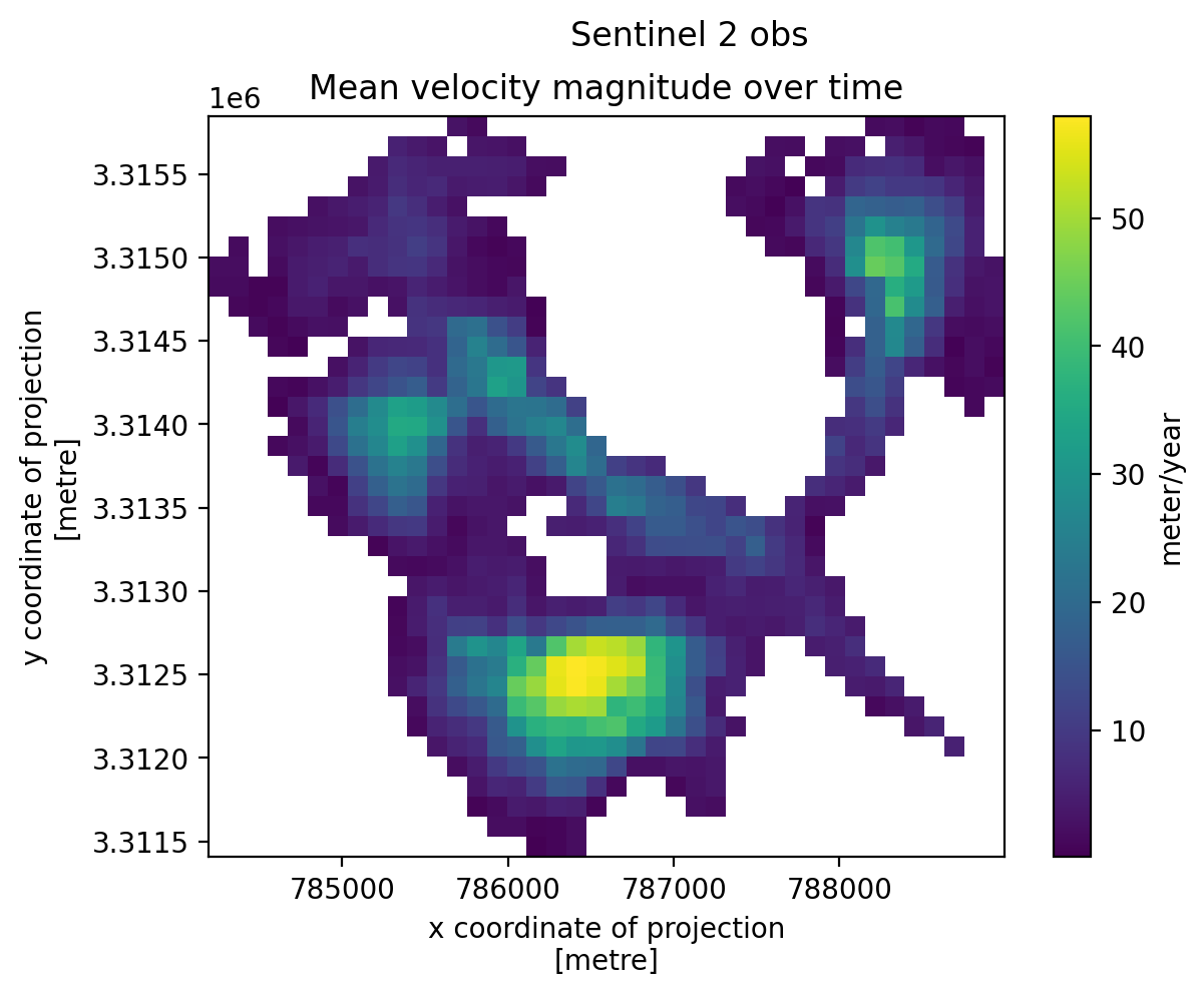
Combine the temporal mean velocities for each sensor into one object#
The plots that we just constructed for each sensor are informative but not great for comparing velocity measurements calculated from each sensor because the colorscales aren’t constant across each sensor. Let’s create a new object that contains the mean magnitude of velocity over time for each sensor and plot them so that they’re easier to compare.
First, we’ll use expand_dims() to add a ‘sensor’ dimension to each dataset and name it appropriately:
l8_mean = l8_mean.expand_dims({'sensor':['L8']})
l7_mean = l7_mean.expand_dims({'sensor':['L7']})
s1_mean = s1_mean.expand_dims({'sensor':['S1']})
s2_mean = s2_mean.expand_dims({'sensor':['S2']})
Next, we want to combine all of these objects together. Xarray has a number of methods for combining data that you can read about here. Because we want to combine the objects along the sensor dimension, xr.concat() is the most appropriate method:
all_sensors = xr.concat([l8_mean,
l7_mean,
s1_mean,
s2_mean], dim='sensor')
all_sensors.sensor
<xarray.DataArray 'sensor' (sensor: 4)> Size: 32B
array(['L8', 'L7', 'S1', 'S2'], dtype=object)
Coordinates:
* sensor (sensor) object 32B 'L8' 'L7' 'S1' 'S2'
spatial_ref int64 8B 0
mapping int64 8B 0- sensor: 4
- 'L8' 'L7' 'S1' 'S2'
array(['L8', 'L7', 'S1', 'S2'], dtype=object)
- sensor(sensor)object'L8' 'L7' 'S1' 'S2'
array(['L8', 'L7', 'S1', 'S2'], dtype=object)
- spatial_ref()int640
- GeoTransform :
- 784192.5 120.0 0.0 3315847.5 0.0 -120.0
array(0)
- mapping()int640
- crs_wkt :
- PROJCS["WGS 84 / UTM zone 46N",GEOGCS["WGS 84",DATUM["WGS_1984",SPHEROID["WGS 84",6378137,298.257223563,AUTHORITY["EPSG","7030"]],AUTHORITY["EPSG","6326"]],PRIMEM["Greenwich",0,AUTHORITY["EPSG","8901"]],UNIT["degree",0.0174532925199433,AUTHORITY["EPSG","9122"]],AUTHORITY["EPSG","4326"]],PROJECTION["Transverse_Mercator"],PARAMETER["latitude_of_origin",0],PARAMETER["central_meridian",93],PARAMETER["scale_factor",0.9996],PARAMETER["false_easting",500000],PARAMETER["false_northing",0],UNIT["metre",1,AUTHORITY["EPSG","9001"]],AXIS["Easting",EAST],AXIS["Northing",NORTH],AUTHORITY["EPSG","32646"]]
- semi_major_axis :
- 6378137.0
- semi_minor_axis :
- 6356752.314245179
- inverse_flattening :
- 298.257223563
- reference_ellipsoid_name :
- WGS 84
- longitude_of_prime_meridian :
- 0.0
- prime_meridian_name :
- Greenwich
- geographic_crs_name :
- WGS 84
- horizontal_datum_name :
- World Geodetic System 1984
- projected_crs_name :
- WGS 84 / UTM zone 46N
- grid_mapping_name :
- transverse_mercator
- latitude_of_projection_origin :
- 0.0
- longitude_of_central_meridian :
- 93.0
- false_easting :
- 500000.0
- false_northing :
- 0.0
- scale_factor_at_central_meridian :
- 0.9996
- spatial_ref :
- PROJCS["WGS 84 / UTM zone 46N",GEOGCS["WGS 84",DATUM["WGS_1984",SPHEROID["WGS 84",6378137,298.257223563,AUTHORITY["EPSG","7030"]],AUTHORITY["EPSG","6326"]],PRIMEM["Greenwich",0,AUTHORITY["EPSG","8901"]],UNIT["degree",0.0174532925199433,AUTHORITY["EPSG","9122"]],AUTHORITY["EPSG","4326"]],PROJECTION["Transverse_Mercator"],PARAMETER["latitude_of_origin",0],PARAMETER["central_meridian",93],PARAMETER["scale_factor",0.9996],PARAMETER["false_easting",500000],PARAMETER["false_northing",0],UNIT["metre",1,AUTHORITY["EPSG","9001"]],AXIS["Easting",EAST],AXIS["Northing",NORTH],AUTHORITY["EPSG","32646"]]
- GeoTransform :
- 784192.5 120.0 0.0 3315847.5 0.0 -120.0
array(0)
- sensorPandasIndex
PandasIndex(Index(['L8', 'L7', 'S1', 'S2'], dtype='object', name='sensor'))
Now we can visualize the temporal averages for each sensor. Note that we use different syntax to specify the colorbar label in this example. Because we are creating a FacetGrid plot object, we don’t use ax objects. Instead we pass the cbar_kwargs dict object:
a = all_sensors.plot(col='sensor', cbar_kwargs={'label':'meters/year'});
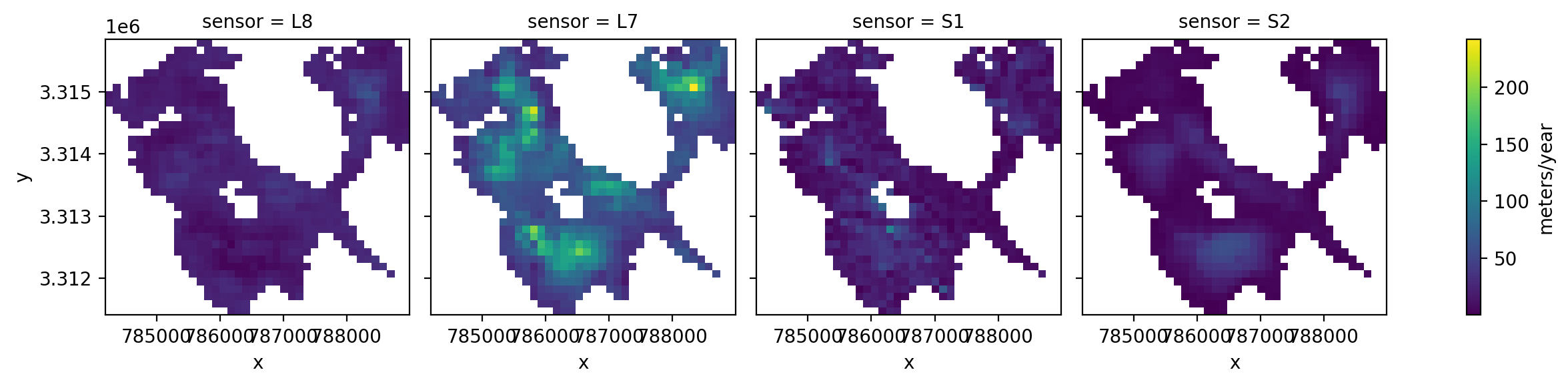
ITS_LIVE is exciting because it combines velocity data from a number of satellites into one accessible and efficient dataset. From this brief look, you can see snapshot overviews of the different data within the dataset and begin to think about processing steps you might take to work with the data further.
Checking coverage along a dimension#
It would be nice to be able to scan/visualize and observe coverage of a variable along a dimension
First need to make a mask that will tell us all the possible ‘valid’ pixels. ie pixels over ice v. rock.
valid_pixels = sample_glacier_raster.v.count(dim=['x','y'])
valid_pix_max = sample_glacier_raster.v.notnull().any('mid_date').sum(['x','y'])
sample_glacier_raster['cov'] = valid_pixels/valid_pix_max
#how many time steps are duplicates?, there are 16872 unique vals in mid_dates
np.unique(sample_glacier_raster['mid_date'].data).shape
(3018,)
Start by grouping over mid_date. Would expect 3,018 (# unique time steps) with mostly groups of 1, groups of more than one on duplicate coords
test_gb = sample_glacier_raster.groupby(sample_glacier_raster.mid_date)
type(test_gb.groups)
dict
test_gb.groups is a dict, so let’s explore that object. The keys correspond to mid_date coordinates (see this for yourself by running test_gb.groups.keys()), so the values should be the entries at that coordinate.
Visualize data coverage over time series#
Let’s take a look at the data coverage over this glacier across the time series:
fig, ax = plt.subplots(figsize=(30,3))
sample_glacier_raster.cov.plot(ax=ax, linestyle='None',marker = 'x')
[<matplotlib.lines.Line2D at 0x7f02d469f610>]
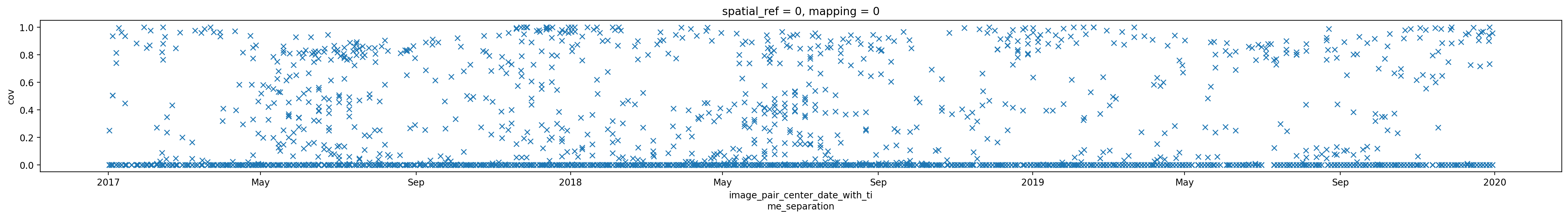
But what if we wanted to explore the relative coverage of the different sensors that make up the its_live dataset as a whole?
We can use groupby to group the data based on a single condition such as satellite_img1 or mid_date.
sample_glacier_raster.cov.groupby(sample_glacier_raster.satellite_img1)
<DataArrayGroupBy, grouped over 1 grouper(s), 5 groups in total:
'satellite_img1': 5/5 groups present with labels '1A', '2A', '2B', '7', '8'>
sample_glacier_raster.groupby('mid_date')
<DatasetGroupBy, grouped over 1 grouper(s), 3018 groups in total:
'mid_date': 3018/3018 groups present with labels 2017-01-01T16:15:50.6605240...>
However, if we want to examine the coverage of data from different sensor groups over time, we would essentially want to groupby two groups. To do this, we use flox
import flox.xarray
This is the xr.DataArray on which we will perform the grouping operation using flox
sample_glacier_raster.cov
<xarray.DataArray 'cov' (mid_date: 3974)> Size: 32kB
array([0.35219236, 0. , 0. , ..., 0. , 0. ,
0. ], shape=(3974,))
Coordinates:
* mid_date (mid_date) datetime64[ns] 32kB 2018-04-14T04:18:49.171219968...
spatial_ref int64 8B 0
mapping int64 8B 0- mid_date: 3974
- 0.3522 0.0 0.0 0.0 0.0 0.0 0.4965 0.0 ... 0.0 0.0 0.0 0.0 0.0 0.0 0.0
array([0.35219236, 0. , 0. , ..., 0. , 0. , 0. ], shape=(3974,)) - mid_date(mid_date)datetime64[ns]2018-04-14T04:18:49.171219968 .....
- description :
- midpoint of image 1 and image 2 acquisition date and time with granule's centroid longitude and latitude as microseconds
- standard_name :
- image_pair_center_date_with_time_separation
array(['2018-04-14T04:18:49.171219968', '2017-02-10T16:15:50.660901120', '2019-03-15T04:15:44.180925952', ..., '2018-06-11T04:10:57.953189888', '2017-05-27T04:10:08.145324032', '2017-05-07T04:11:30.865388288'], shape=(3974,), dtype='datetime64[ns]') - spatial_ref()int640
- GeoTransform :
- 784192.5 120.0 0.0 3315847.5 0.0 -120.0
array(0)
- mapping()int640
- crs_wkt :
- PROJCS["WGS 84 / UTM zone 46N",GEOGCS["WGS 84",DATUM["WGS_1984",SPHEROID["WGS 84",6378137,298.257223563,AUTHORITY["EPSG","7030"]],AUTHORITY["EPSG","6326"]],PRIMEM["Greenwich",0,AUTHORITY["EPSG","8901"]],UNIT["degree",0.0174532925199433,AUTHORITY["EPSG","9122"]],AUTHORITY["EPSG","4326"]],PROJECTION["Transverse_Mercator"],PARAMETER["latitude_of_origin",0],PARAMETER["central_meridian",93],PARAMETER["scale_factor",0.9996],PARAMETER["false_easting",500000],PARAMETER["false_northing",0],UNIT["metre",1,AUTHORITY["EPSG","9001"]],AXIS["Easting",EAST],AXIS["Northing",NORTH],AUTHORITY["EPSG","32646"]]
- semi_major_axis :
- 6378137.0
- semi_minor_axis :
- 6356752.314245179
- inverse_flattening :
- 298.257223563
- reference_ellipsoid_name :
- WGS 84
- longitude_of_prime_meridian :
- 0.0
- prime_meridian_name :
- Greenwich
- geographic_crs_name :
- WGS 84
- horizontal_datum_name :
- World Geodetic System 1984
- projected_crs_name :
- WGS 84 / UTM zone 46N
- grid_mapping_name :
- transverse_mercator
- latitude_of_projection_origin :
- 0.0
- longitude_of_central_meridian :
- 93.0
- false_easting :
- 500000.0
- false_northing :
- 0.0
- scale_factor_at_central_meridian :
- 0.9996
- spatial_ref :
- PROJCS["WGS 84 / UTM zone 46N",GEOGCS["WGS 84",DATUM["WGS_1984",SPHEROID["WGS 84",6378137,298.257223563,AUTHORITY["EPSG","7030"]],AUTHORITY["EPSG","6326"]],PRIMEM["Greenwich",0,AUTHORITY["EPSG","8901"]],UNIT["degree",0.0174532925199433,AUTHORITY["EPSG","9122"]],AUTHORITY["EPSG","4326"]],PROJECTION["Transverse_Mercator"],PARAMETER["latitude_of_origin",0],PARAMETER["central_meridian",93],PARAMETER["scale_factor",0.9996],PARAMETER["false_easting",500000],PARAMETER["false_northing",0],UNIT["metre",1,AUTHORITY["EPSG","9001"]],AXIS["Easting",EAST],AXIS["Northing",NORTH],AUTHORITY["EPSG","32646"]]
- GeoTransform :
- 784192.5 120.0 0.0 3315847.5 0.0 -120.0
array(0)
- mid_datePandasIndex
PandasIndex(DatetimeIndex(['2018-04-14 04:18:49.171219968', '2017-02-10 16:15:50.660901120', '2019-03-15 04:15:44.180925952', '2019-07-20 16:15:55.190603008', '2018-01-31 16:15:50.170811904', '2017-12-17 16:15:50.170508800', '2017-10-16 04:18:49.170811904', '2017-11-27 16:20:45.171105024', '2017-10-08 16:17:55.170906112', '2019-10-23 16:18:15.191001088', ... '2017-10-06 04:11:40.987761920', '2018-03-31 04:10:01.464065024', '2018-06-11 04:09:32.921265664', '2017-07-26 04:11:49.029760256', '2017-04-21 04:11:32.560144896', '2017-09-12 04:11:46.053865984', '2017-06-24 04:11:18.708142080', '2018-06-11 04:10:57.953189888', '2017-05-27 04:10:08.145324032', '2017-05-07 04:11:30.865388288'], dtype='datetime64[ns]', name='mid_date', length=3974, freq=None))
Using flox, we will define a coverage object that takes as inputs the data we want to reduce, the groups we want to use to group the data and the reduction we want to perform.
coverage = flox.xarray.xarray_reduce(
# array to reduce
sample_glacier_raster.cov,
# Grouping by two variables
sample_glacier_raster.satellite_img1.compute(),
sample_glacier_raster.mid_date,
# reduction to apply in each group
func="mean",
# for when no elements exist in a group
fill_value=0,
)
Now we can visualize the coverage over time for each sensor in the its_live dataset. Cool!
plt.pcolormesh(coverage.mid_date, coverage.satellite_img1, coverage, cmap='magma')
plt.colorbar();

Conclusion#
This notebook displayed basic data inspection steps that you can take when working with a new dataset. The following notebooks will demonstrate further processing, analytical and visualization steps you can take. We will be working with the same object in the following notebook, so we can use cell magic to store the object and read it in in the next notebook, rather than making it all over again. You can read more about the magic command here.
%store sample_glacier_raster
Stored 'sample_glacier_raster' (Dataset)